Scalar Quantization with Random Thresholds
Abstract
The distortion–rate performance of certain randomly-designed scalar quantizers is determined. The central results are the mean-squared error distortion and output entropy for quantizing a uniform random variable with thresholds drawn independently from a uniform distribution. The distortion is at most 6 times that of an optimal (deterministically-designed) quantizer, and for a large number of levels the output entropy is reduced by approximately bits, where is the Euler–Mascheroni constant. This shows that the high-rate asymptotic distortion of these quantizers in an entropy-constrained context is worse than the optimal quantizer by at most a factor of .
Index Terms:
Euler–Mascheroni constant, harmonic number, high-resolution analysis, quantization, Slepian–Wolf coding, subtractive dither, uniform quantization, Wyner–Ziv coding.I Introduction
What is the performance of a collection of subtractively-dithered uniform scalar quantizers with the same step size, used in parallel? The essence of this question—and a precise analysis under high-resolution assumptions—is captured by answering another fundamental question: What is the mean-squared error (MSE) performance of a -cell quantizer with randomly-placed thresholds applied to a uniformly-distributed source? For both (equivalent) questions, it is not obvious a priori that the performance penalties relative to optimal deterministic designs are bounded; here we find concise answers that demonstrate that these performance penalties are small. Specifically, the multiplicative penalty in MSE for quantization of a uniform source is at most in the codebook-constrained case and about in the entropy-constrained case at high rate, where is the Euler–Mascheroni constant [1]. The translation of these results is that the multiplicative penalty in MSE for high-rate parallel dithered quantization is at most when there is no expoitation of statistical dependencies between channels and about when joint entropy coding or Slepian–Wolf coding [2] is employed and the number of channels is large.
Quantization with parallel channels is illustrated in Fig. 1. Each of quantizers is a subtractively-dithered uniform scalar quantizer with step size . Denoting the dither, or offset, of quantizer by , the thresholds of the quantizer are . One may imagine several stylized applications in which it is advantageous to allow the s to be arbitrary or chosen uniformly at random. For example, with parallel quantizer channels, one may turn channels on and off adaptively based on available power or the desired signal fidelity [3]. Alteration of the lossless coding block could then be achieved through a variety of means [4, 5, 6]. The same figure could represent a distributed setting, in which sensors measure highly-correlated quantities (all modeled as ); with a Slepian–Wolf code [2] or universal Slepian–Wolf code [7], the sensors can quantize and encode their samples autonomously. Variations in the s could also arise unintentionally, through process variation in sensor manufacturing due to cost reduction or size reduction; mitigation of process variations is expected to be of increasing importance [8]. This letter addresses the performance loss relative to deterministic joint design of the channels or coordinated action by the distributed sensors.
-2.5,-1)(8.5,4.5)
Collectively, the parallel quantizers specify input with thresholds . One would expect the best performance from having uniformly spaced in through ; this intuition is verified under high-resolution assumptions, where the optimal entropy-constrained quantizers are uniform [9]. To analyze performance relative to this ideal, it suffices to study one interval of length in the domain of the quantizers because the thresholds repeat with a period of . This analysis is completed in Section II. The ramifications for the system in Fig. 1 are made explicit in Section III. Section IV considers uniform quantizers with unequal step sizes, and Section V provides additional connections to related results and concludes the note.
II Random Quantizer for a Uniform Source
Let be uniformly distributed on . Suppose that a -level quantizer for is designed by choosing thresholds independently, each with a uniform distribution on . Put in ascending order, the random thresholds are denoted , and for notational convenience, let and . A regular quantizer with these thresholds has lossy encoder given by
The optimal reproduction decoder for MSE distortion is given by
We are interested in the average rate and distortion of this random quantizer as a function of , both with and without entropy coding.
Theorem 1
The MSE distortion, averaging over both the source variable and the quantizer thresholds , is
| (1) |
Proof:
Let denote the length of the quantizer partition cell that contains when the random thresholds are ; i.e., L(x — {a_k}_k=1^K-1) = length(α^-1(α(x))). Since is uniformly distributed and the thresholds are independent of , the quantization error is conditionally uniformly distributed for any values of the thresholds. Thus the conditional MSE given the thresholds is , and averaging over the thresholds as well gives .
The possible values of the interval length, , are called spacings in the order statistics literature [10, Sect. 6.4]. With a uniform parent distribution, the spacings are identically distributed. Thus they have the distribution of the minimum, : f_a_1(a) = (K-1)(1-a)^K-2, 0 ≤a ≤1. The density of is obtained from the density of by noting that the probability that falls in an interval is proportional to the length of the interval: f_L(ℓ) = ℓf a 1 (ℓ) ∫ 0 1 ℓf a 1 (ℓ) dℓ = K(K-1) ℓ(1-ℓ)^K-2, for . Now
completing the proof. An alternative proof is outlined in the Appendix. ∎
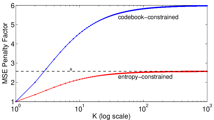
The natural comparison for (1) is against an optimal -level quantizer for the uniform source. The optimal quantizer has evenly-spaced thresholds, resulting in partition cells of length and thus MSE distortion of . Asymptotically in , Distortion (1) is worse by a factor of , which is at most and approaches as . In other words, designing a codebook-constrained or fixed-rate quantizer by choosing the thresholds at random creates a multiplicative distortion penalty of at most 6.
Now consider the entropy-constrained or variable-rate case. If an entropy code for the indexes is designed without knowing the realization of the thresholds, the rate remains bits per sample. However, conditioned on knowing the thresholds, the quantizer index is not uniformly distributed, so the performance penalty can be reduced.
Theorem 2
The expected quantizer index conditional entropy, averaging over the quantizer thresholds , is
| (2) |
Proof:
The desired expected conditional entropy is the expectation of the self-information, . Let be defined as in the proof of Theorem 1 to be the length of the interval containing . Since the probability of falling into any subinterval of of length is , we have
which equals (2) by direct calculation; see also [11],[12, 4.6]. An alternative proof is outlined in the Appendix. ∎
To compare again against an optimal -level quantizer, note that evenly-spaced thresholds would yield while the rate in (2) is also essentially logarithmic in . The quantity (2) includes the harmonic number , which has been studied extensively. For example,
where is called the Euler–Mascheroni constant [1].
Combining (1) and (2) while exploiting the asymptotic approximation yields
and a distortion–rate performance of
| (3) |
where represents a ratio approaching 1 as increases for distortions and difference approaching 0 as increases for rates. The exact performance from (1)–(2) is shown in Fig. 2 with normalization through division by .
III Parallel Dithered Quantizers
Let us now return to the system depicted in Fig. 1. High-resolution analysis of this system for any number of channels follows easily from the results of the previous section.
For notational convenience, let us assume that the source has a continuous density supported on . Fix and consider uniform quantizers with step size applied to . Quantizer has lossy encoder with thresholds at integer multiples of . The remaining quantizers are offset by , i.e., the thresholds of Quantizer with lossy encoder are at .
We would like to first approximate the distortion in joint reconstruction from . The first quantizer index isolates to an interval of length . Since has a continuous density and , we may approximate as conditionally uniformly distributed on this interval. Thus we may apply Theorem 1 to obtain
| (4) |
where represents a ratio approaching 1 as . The average of the joint entropy is increased from (2) by precisely . Since
where is the differential entropy of [13],
| (5) |
where represents a difference approaching 0 as . For a large number of channels , eliminating gives
| (6) | |||||
where (a) is exact as , (b) is the standard approximation for harmonic numbers, and (c) is an approximation for large . This distortion exceeds the distortion of optimal entropy-constrained quantization by the factor .
IV Quantizers with Unequal Step Sizes
The methodology introduced here can be extended to cases with unequal quantizer step sizes. The details become quickly more complicated as the number of distinct step sizes is increased, so we consider only two step sizes. We also limit attention to source uniformly distributed on .
Let quantizer be a uniform quantizer with step size and thresholds at integer multiples of (no offset). Let be a uniform quantizer with step size and thresholds offset by , where is uniformly distributed on . Without loss of generality, assume . (It does not matter which quantizer is fixed to have no offset; it only simplifies notation.)
Mimicking the analysis in Section II, the performance of this pair of quantizers is characterized by the p.d.f. of the length of the partition cell into which falls. Furthermore, because of the random dither , the partition cell lengths are identically distributed.
Let be the length of the partition cell with left edge at . Clearly is related to by
| (7) |
So is a mixed random variable with (generalized) p.d.f.
With defined (as before) as the length of the partition cell that contains ,
for . The average distortion is given by
| (8) |
This expression reduces to (4) (with ) for . Also, it approaches as consistent with the second quantizer providing no information. The average rate is
| (9) |
This reduces to (5) (with and ) for .
One way in which unequal quantization step sizes could arise is through the quantization of a frame expansion [14]. Suppose the scalar source is encoded by dithered uniform scalar quantization of with step size for each component of . This is equivalent to using quantizers with step sizes
directly on . Fixing so that , we can express the distortion (8) as
and the rate (9) as
The quotient
| (10) |
can be interpreted as the multiplicative distortion penalty as compared to using a single uniform quantizer. This is bounded above by
which is consistent with evaluating (6) at . Thus, joint entropy coding of the quantized components largely compensates for the (generally disadvantageous) expansion of into a higher-dimensional space before quantization; the penalty is only an distortion factor or bits.
V Discussion
This note has derived distortion–rate performance for certain randomly-generated quantizers. The thresholds (analogous to offsets in a dithered quantizer) are chosen according to a uniform distribution. The technique can be readily extended to other quantizer threshold distributions; however, the uniform distribution is motivated by the asymptotic optimality of uniform thresholds in entropy-constrained quantization.
The analysis in Section III puts significant burden on the entropy coder to remove the redundancies in the quantizer outputs . This is similar in spirit to the universal coding scheme of Ziv [15], which employs a dithered uniform scalar quantizer along with an ideal entropy coder to always perform within 0.754 bits per sample of the rate–distortion bound. In the case that the quantizers are distributed, we are analyzing the common strategy for Wyner–Ziv coding [16] of quantizing followed by Slepian–Wolf coding; we obtain a concrete rate loss upper bound of bits per sample when the rate is high; this is approached when the number of encoders is large. With non-subtractive dither, the randomization of thresholds is unchanged but the reproduction points are not matched to the thresholds. Thus, the rate computation is unchanged but distortions are increased.
Use of analog-to-digital converter channels with differing quantization step sizes was studied in [17]. Unlike the present note, this work exploits correlation of a wide-sense stationary input; however, it is limited by a simple quantization noise model and estimation by linear, time-invariant (LTI) filtering.
Exact MSE analysis of quantized overcomplete expansions has proven difficult, so many papers have focused on only the scaling of distortion with the redundancy of the frame [18, 19, 14, 20]. The example in Section IV, could be extendable to more general frame expansions.
The proofs of Theorems 1 and 2 are indirect in that they introduce the random variable for the length of the partition cell containing . A more direct proof is outlined here.
Lemma 1
For fixed thresholds ,
Proof:
The quantizer maps interval to so P(α(X) = k — {a_j}_j=1^K-1 ) = a_k - a_k-1. The entropy expression is thus immediate. The distortion expression follows by expanding the expectation using the law of total expectation with conditioning on :
∎
The theorems are proved by averaging over the joint distribution of the quantizer thresholds , which is uniform over the simplex .
Acknowledgments
The author is thankful to John Sun, Lav Varshney, and an anonymous reviewer for helpful suggestions.
References
- [1] J. Havil, Gamma: Exploring Euler’s Constant. Princeton, NJ: Princeton University Press, 2003.
- [2] D. Slepian and J. K. Wolf, “Noiseless coding of correlated information sources,” IEEE Trans. Inform. Theory, vol. IT-19, no. 4, pp. 471–480, Jul. 1973.
- [3] A. P. Chandrakasan, S. Sheng, and R. W. Brodersen, “Low-power CMOS digital design,” IEEE J. Solid-State Circuts, vol. 27, no. 4, pp. 473–484, Apr. 1992.
- [4] J. Ziv and A. Lempel, “A universal algorithm for sequential data compression,” IEEE Trans. Inform. Theory, vol. IT-23, no. 3, pp. 337–343, May 1977.
- [5] J. G. Cleary and I. H. Witten, “Data compression using adaptive coding and partial string matching,” IEEE Trans. Commun., vol. 32, no. 4, pp. 396–402, Apr. 1984.
- [6] I. H. Witten, R. M. Neal, and J. G. Cleary, “Arithmetic coding for data compression,” Comm. ACM, vol. 30, no. 6, pp. 520–540, Jun. 1987.
- [7] Y. Oohama and T. S. Han, “Universal coding for the Slepian–Wolf data compression system and the strong converse theorem,” IEEE Trans. Inform. Theory, vol. 40, no. 6, pp. 1908–1919, Nov. 1994.
- [8] “International technology roadmap for semiconductors,” 2010 Update, online: itrs.net.
- [9] H. Gish and J. P. Pierce, “Asymptotically efficient quantizing,” IEEE Trans. Inform. Theory, vol. IT-14, no. 5, pp. 676–683, Sep. 1968.
- [10] H. A. David and H. N. Nagaraja, Order Statistics, 3rd ed. Hoboken, NJ: John Wiley & Sons, 2003.
- [11] N. Ebrahimi, E. S. Soofi, and H. Zahedi, “Information properties of order statistics and spacings,” IEEE Trans. Inform. Theory, vol. 50, no. 1, pp. 177–183, Jan. 2004.
- [12] L. R. Varshney, “Optimal information storage: Nonsequential sources and neural channels,” Master’s thesis, Massachusetts Inst. of Tech., Cambridge, MA, Jun. 2006.
- [13] A. Rényi, “On the dimension and entropy of probability distributions,” Acta Math. Acad. Sci. Hungar., vol. 10, pp. 193–215, 1959.
- [14] V. K. Goyal, M. Vetterli, and N. T. Thao, “Quantized overcomplete expansions in : Analysis, synthesis, and algorithms,” IEEE Trans. Inform. Theory, vol. 44, no. 1, pp. 16–31, Jan. 1998.
- [15] J. Ziv, “On universal quantization,” IEEE Trans. Inform. Theory, vol. IT-31, no. 3, pp. 344–347, May 1985.
- [16] A. D. Wyner and J. Ziv, “The rate-distortion function for source coding with side information at the decoder,” IEEE Trans. Inform. Theory, vol. IT-22, no. 1, pp. 1–10, Jan. 1976.
- [17] S. Maymon and A. V. Oppenheim, “Quantization and compensation in sampled interleaved multi-channel systems,” in Proc. IEEE Int. Conf. Acoust., Speech, and Signal Process., Dallas, TX, Mar. 2010.
- [18] N. T. Thao and M. Vetterli, “Deterministic analysis of oversampled A/D conversion and decoding improvement based on consistent estimates,” IEEE Trans. Signal Process., vol. 42, no. 3, pp. 519–531, Mar. 1994.
- [19] ——, “Lower bound on the mean-squared error in oversampled quantization of periodic signals using vector quantization analysis,” IEEE Trans. Inform. Theory, vol. 42, no. 2, pp. 469–479, Mar. 1996.
- [20] S. Rangan and V. K. Goyal, “Recursive consistent estimation with bounded noise,” IEEE Trans. Inform. Theory, vol. 47, no. 1, pp. 457–464, Jan. 2001.