Coordinate rings for the moduli stack of quasi-parabolic principal bundles on a curve and toric fiber productsThanks: This work was supported by the NSF fellowship DMS-0902710
Abstract.
We continue the program started in [M1] to understand the combinatorial commutative algebra of the projective coordinate rings of the moduli stack of quasi-parabolic principal bundles on a generic marked projective curve. We find general bounds on the degrees of polynomials needed to present these algebras by studying their toric degenerations. In particular, we show that the square of any effective line bundle on this moduli stack yields a Koszul projective coordinate ring. This leads us to formalize the properties of the polytopes used in proving our results by constructing a category of polytopes with term-orders. We show that many of results on the projective coordinate rings of follow from closure properties of this category with respect to fiber products.
1. Introduction
We wish to understand the structure of the projective coordinate rings of the moduli stack of quasi-parabolic principal bundles on a marked projective curve where is a simple complex group and the parabolic structure is given by a Borel subgroup Our interest in these objects stems both from the classical value of problems in the moduli of bundles, and because the graded components of these algebras can be identified with spaces of conformal blocks. Conformal blocks for the conformal field theory defined by a simple complex Lie algebra and a non-negative integer for marked projective complex curves occupy an interesting position in algebraic geometry and mathematical physics. When the curve is allowed to vary, they form vector bundles over which have been the object of interesting recent work, [F], [AGS]. When the genus of the curve is set to they are the structure spaces for a category of representations of the specialization of a quantum group at a root of unity. As we will mention below, their combinatorics have even made appearances in mathematical biology. Because of the variety of applications, we seek to understand structural features of conformal blocks, and relate them to the commutative algebra of .
The moduli stack can be expressed as the quotient stack of a product of the affine Grassmannian variety with the projective variety by an action of an ind-group determined by the points
| (1) |
The Picard group of calculated in [LS], is a product of copies of the character group of times a copy of
| (2) |
The cone of line bundles with non-zero global sections is a subcone of where is the Weyl chamber of The space of global sections for a vector of dominant weights of and a non-negative integer agrees with the space of conformal blocks of the rational conformal field theory defined by and with weights at the marked points and level Let be the projective coordinate ring of defined by
| (3) |
The Hilbert function of this algebra outputs the sequence of dimensions of the spaces of conformal blocks associated to which can be calculated by the Verlinde formula from conformal field theory, see [B]. These algebras have been studied before, predominantly in the case when is empty. In this case, elements of are known as non-abelian theta functions, and the map to projective space on the coarse moduli space defined by is known as the theta-map. We direct the reader to the article [P] for a survey of what is known about this ring. For , the ring of non-abelian Theta functions has also recently been shown to be projectively normal by Abe, [A]. The present paper is in part motivated by an attempt to extend understanding to the parabolic case, when is non-empty.
The algebra is defined as above only for smooth, however the space makes sense for any stable curve In [M2], we showed that the direct sum can be given an algebra structure for any stable curve, and over smooth curves this agrees with the algebra structure on From now on we refer to these fibers for a non-smooth curve with the same notation. Additionally, these algebras fit together into a flat sheaf of algebras over This implies that one can deduce properties of for generic by studying the algebra for a particular Our strategy is to deduce properties about by passing to the fiber over non-smooth curves in where the combinatorics of the factorization rules (see [TUY], [B]) of conformal blocks can help.
1.1. Conformal blocks as weighted graphs
The stack is stratified by closed substacks indexed by graphs The lowest components of this stratification are certain closed points indexed by trivalent graphs with first Betti number and leaves. The curve corresponding to a trivalent graph is the stable arrangement of marked copies of with dual graph

We now restrict our attention to For this group, dominant weights are non-negative integers In this case, the factorization rules imply that the space of conformal blocks over the point corresponding to a graph has a distinguished basis given by weightings of the edges of by non-negative integers which satisfy a short collection of conditions.
Definition 1.1.
For a trivalent graph with leaves labeled an vector of non-negative integers, and we define to be the set of non-negative real weightings of the edges of which satisfy the following conditions.
- (1)
For any trinode with the three incident edge weights must satisfy the triangle inequalities:
- (2)
For any trinode as above,
- (3)
The weight on the edge attached to the th leaf equals

We consider this polytope with respect to the lattice of integer points in defined by the condition that the sum for any trinode In addition to indexing a basis of the spaces the polytope captures more information about the algebras in the sense that the edge-wise addition operation on weightings of is almost the same as the multiplication operation in these algebras. The following is proved in [StX] for genus and for general genus by Proposition of [M2].
Theorem 1.2.
Let be a trivalent graph with labeled leaves and first Betti number equal to For any curve the algebra can be flatly degenerated to the graded semigroup algebra associated to
Proof.
Both steps, establishing the flat sheaf of algebras over and defining and analyzing the ordering, appear in [M2],( see also [A]). For any curve the algebra is in a flat family with the algebra over the curve of type by Proposition of [M2]. By analyzing with respect to the distinguished basis given by the factorization rules, it can be found that multiplication in this algebra is ”lower triangular” with respect to a natural ordering on the weightings of That is, if and are the elements of corresponding to weightings then Taking the associated graded algebra of with respect to this term order then yields the graded toric algebra A standard Reese algebra construction then yields a flat family over with general fiber and special fiber ∎
The conditions satisfied by the weights around each internal vertex are called the quantum Clebsch-Gordon conditions. Weightings of graphs which satisfy these conditions are known by various names in mathematical physics, such as Feynman diagrams or spin diagrams, see [Ko]. Analysis of these polytopes and other convex sets of spin diagrams also appears in computational biology, specifically in the work of Buczynska and Wiesniewski on phylogenetic algebraic varieties, [BW], [Bu]. The polytope is a cross-section of the cone corresponding to Buczynska’s graphical phylogenetic toric variety introduced in [Bu] to study the Jukes-Cantor statistical model on graphs.
A good deal of information is preserved by flat degeneration, such as the degree, the Hilbert function of and commutative algebra features like the Gorenstein property. In theory, all of these details can be computed from the polytopes A non-trivial consequence of this observation is that the equivalent polyhedral information for the volume and the number of lattice points, etc, is independent of the graph It should be noted that the degeneration technique we are using here applies to other groups as well, except the resulting degenerations are not toric. Perhaps this issue can be resolved with a better understanding of the underlying combinatorial representation theory.
1.2. Statement of results
Depending on the property of one wishes to study, certain toric degenerations can be more suited to the task than others. Next we describe the conditions we place on with respect to in order to ensure the polytope is suited to our needs. We will use three special graph topologies, depicted in Figure 3.
Definition 1.3.
A trivalent tree is said to be if every vertex is connected by an edge to some leaf.
Notice that a caterpillar tree has two pairs of leaves which share a common vertex. We call these paired leaves, and we say they are at the head or tail of the caterpillar.
Definition 1.4.
A trivalent graph is said to be a caterpillar graph if it is obtainable from a caterpillar tree by adding a loop on one of the leaves at the head or tail, or by adding a doubled edge at the midpoint of one of the edges.
Definition 1.5.
A trivalent graph of genus with leaves is if it is obtained from a trivalent tree with leaves by adding loops on leaves.

In our analysis of for tree-like, we require that and satisfy a condition, which we call compatibility.
Definition 1.6.
For the polytope we say a vector is ”compatible” with a graph if any odd is assigned to a leaf-edge which shares a vertex with with the leaf-edge of another odd

Recall that for any lattice point in , the weights at any trinode of sum to an even number. It is a simple combinatorial exercise to show that this implies that the number of odd-weighted leaf-edges of is always even. As a consequence, we obtain that there are only conformal blocks with weights if an even number of the are odd, this implies the following.
Proposition 1.7.
Whenever has dimension there is a tree-like graph which is compatible with
The compatibility property was critical in the proof of the following theorem, from [M1].
Theorem 1.8.
Let be a trivalent tree, and , and let be compatible with then is generated in degree and the binomial ideal of relations is generated by polynomials of degree
Our first result is a generalization of Theorem 1.8 to tree-like graphs.
Theorem 1.9.
Let be tree-like, and and compatible with then is generated in degree and the binomial ideal of relations is generated by polynomials of degree
In [M1] there are examples which show that certain degree polynomials are necessary to generate However, when we choose to have the caterpillar graph topology, the relations can become more tractable.
Theorem 1.10.
Let be a caterpillar graph, then is generated in degree and the presenting ideal has a quadratic, square-free Gröbner basis.
A consequence is that any non-empty becomes ”nice” (normal, with quadratically generated binomial ideal) when we take its Minkowski square, Using the flat degeneration, these theorems can be lifted back to the algebras
Theorem 1.11.
For any , , and a generic curve, is generated in degree with ideal of relations generated in degree For any , is Koszul. In particular, it has quadratic relations.
Proof.
We give a sketch of the argument. Let and be compatible. We assume that both properties have been proved for the appropriate toric algebra This implies the corresponding statements for the fiber by standard properties of associated graded algebras. The moduli is a connected, Noetherian Deligne-Mumford stack over therefore for any closed point there is a dense open substack with an étale Noetherian affine cover The fiber of our sheaf of algebras is then equal to the fiber of the pullback sheaf over for some closed point of
Over a Noetherian affine base, we obtain the statement on generators and relations from an application of Nakayama’s lemma to the graded components of the algebra and its presenting ideal. The statement on the Koszul property results from the fact that Betti numbers of the corresponding generalized Koszul complex (see [E], Ex ) do not increase under specialization because their graded components are locally free modules. We may reduce to this case because the generic point of is étale-covered by the generic point of and the fiber over this point is obtained by base-change.
∎
Remark 1.12.
Naturally, this theorem applies in the case when is empty. In this case it implies that the above generation and relation properties hold for the projective coordinate ring of the square of the line bundle on for generic The generation result is weaker than the result of Abe, [A], however the result on relations is new. Abe’s strategy is similar to ours, he employs a filtration built from the factorization rules, however he stops short of a toric degeneration. It is at present unknown to us if Abe’s results can be replicated with an inspired choice of graph
Remark 1.13.
When is a tree and is very large, the algebra is also realized as a toric degeneration of a projective coordinate ring of the moduli of -weighted points on the projective line, Theorem 1.10 then shows that this projective coordinate ring has a quadratic, square-free Gröbner basis when is even, a result also obtained by Herring and Howard, [HH].
1.3. Building blocks of
Theorems 1.8 ,1.9, and 1.10 are proved by understanding the structure of as a fiber product of rational polytopes. In [M1], the polytopes for a trivalent tree were shown to be ”balanced,” a geometric feature which endows a polytope with several nice algebraic properties. The technical observation that makes these theorems work is the fact that the balanced property is stable with respect to certain kinds of fiber products.
Definition 1.14.
Let , and be lattice polytopes, and let and be lattice maps which take into The fiber product is defined to be the subset of points such that
We will prove Theorem 1.9 by following a similar strategy to the program used in [M1]. The conditions which define are all localized around individual trinodes of which implies we may represent as a fiber product of polytopes defined on the components of an ”exploded graph” This is a graph obtained from by splitting any edge in which separates the graph into two disjoint components.

See also Figure 14. The connected components of each have a special polytope associated to them, we call these the ”building blocks” of The strategy is to first analyze the building block polytopes, establishing that they have the algebraic features we want, then show these features are stable under fiber product. When is tree-like, the polytopes given by weightings of the components of are single loops with an edge, or a trinode with , , or edges with edge weight fixed to a specific value (say or ). When is caterpillar, no trinodes with fixed edges appear, but a loop with edges can appear, see Figure 6 below. There is a depiction of each polytope beneath its corresponding graph. See Figures 10, 7, 8, and 9 for more detailed illustrations of these polytopes.

We call the polytope corresponding to a loop with an edge weightings of a trinode with one or two fixed edges (with value equal to ) or respectively, general weightings of a trinode and a loop with two edges The polytope is dimensional, so the image depicted in the figure is a projection into
Here is where compatibility and the assumption that we work with even level are used. It is another simple combinatorial exercise to verify that when are compatible, all non-leaf and non-loop edges of are weighted with an even number. This greatly simplifies the structure of the building block polytopes. The main technical part of this paper is to develope and clarify the polytope properties that make this construction work. As fiber products are categorical operations, we view the natural habitat for the above theorems as closure properties of a category of polytopes under certain fiber products. We define this category next.
1.4. The category
For the following definitions see [St]. For a lattice polytope let be an assignment of real numbers to the lattice points of The function defines a term order on the polynomial ring For a monomial we define For two monomials, we say when or and
The polytope defines a graded algebra where the th graded component has a basis given by the lattice points of the -th minkowski sum and the product operation is lattice point addition. Let be the toric ideal which is the kernel of the map For a polynomal the initial form with respect to is defined to be the sum of the monomials in which are largest under the term order defined by
Definition 1.15.
A monomial is said to be standard with respect to a term order if it is an initial form of any polynomial in
For a lattice point we let be the set of monomials in which map to The difference of any two elements in is a member of The function defines a partial ordering on and the minimal elements of this partial ordering are the standard monomials.
Definition 1.16.
We define the category to have pairs as objects, where is a lattice polytope in some and is a term order on . A morphism is a linear map on induced by a map on lattices, such that the standard monomials of map to standard monomials of
The following is the most general result we will prove about the category We say has unique standard monomials if the sets always have a unique minimal element when they are non-empty.
Proposition 1.17.
If and are maps in and if has unique standard monomials, then the fiber product object exists in
The category of lattice polytopes comes with a fiber product, so the content of this proposition is in showing that there is a term order on with maps to , satisfying the universal property of a fiber product. Next, we formalize properties of balanced polytopes first observed in [M1] by showing that the category has a distinguished subcategory that is closed under fiber product.
Definition 1.18.
A term order on a lattice polytope is said to be ”flag” when a monomial from is standard if and only if every degree divisor of is standard, and is standard for any .
Proposition 1.19.
If and are maps in and if has unique standard monomials, then and flag implies flag.
Balanced polytopes are examples of polytopes with flag term orders. Geometrically, the term order divides the polytope into sub-polytopes, and the standard monomials are simply monomials with components all corresponding to lattice points from the same sub-polytope, called a ”standard region.” In the case of balanced polytopes, these regions are all lattice sub-polytopes of the unit cube. Theorem 1.9 above is a consequence of the following propositions. Recall that a rational lattice polytop is said to be when the graded algebra is generated in degree by the elements corresponding to the lattice points of
Proposition 1.20.
Let be a fiber product of flag elements over with unique standard monomials. If each is normal, then is normal.
For we call a binomial a standard relation if both monomials are composed of lattice points from the same standard region.
Proposition 1.21.
Let be a fiber product of flag objects over with unique standard monomials. If the standard relations of are generated by standard relations of degree then is generated in degree
Properties of fiber products over a toric algebra have been studied before by Sullivant in [Su]. These theorems can be viewed as refinements of Theorem 2.8 in [Su]. In our results, the assumption that the base of the fiber product have strict unique factorization has been removed by restricting our study to fiber products of binomial ideals.
1.5. The concatenation product on term orders
The second technical result, used to prove theorem 1.10, is a version of Sullivant’s Theorem 2.9 in [Su]. Here we also remove a restriction that the base of the fiber product have unique factorization by only considering binomial ideals. We define another operation in
Definition 1.22.
Define in on the fiber product polytope with term order given by the following rule on monomials. For lattice points we say if
- (1)
or
- (2)
the values are equal, and
For monomials we first order by degree, then with the sum weighting we then break ties by writing both sets of exponents in decreasing order with the above ordering and we declare if at the first place they differ.
Proposition 1.23.
If the presenting ideals of and all have quadratic, square-free Gröbner bases with respect to their term orders, then so does the presenting ideal of
Using this, we establish Theorem 1.10 from the fact that the presenting ideals of intervals and the building block polytopes have quadratic, square-free Gröbner bases. Note that although we do not assume that the base of our fiber products has unique factorization, we do assume this ”locally” by requiring the polytope to have a quadratic square-free Gröbner basis.
1.6. Acknowledgements
We would like to thank Weronika Buczynska, Anton Dochtermann, Alex Engström, Ben Howard, Raman Sanyal, and Seth Sullivant for useful conversations related to this project, and David Eisenbud for his helpful explanations of the behavior of graded algebras in flat families. We also thank the reviewer, who pointed us to the work of Abe [A], the result of which was inspiration for stronger results than we originally appeared in this paper.
2. The category and flag term orders
In this section we review some basic properties of term orders on toric ideals. We discuss geometric decompositions of the polytope induced by a term order, and the corresponding algebra We cover some properties of the category flag term orders, and balanced polytopes. First, we recall the initial complex of a term order, see chapter of [St].
Definition 2.1.
Let be a lattice polytope, and a term order on Define the simplicial complex on the vertex set as follows. A set defines a face of if every monomial with support is standard.
If and has a monomial supported on its entries which is not standard then one can make a non-standard monomial supported on by multiplying by the remaining generators in this establishes that is a simplicial complex. Morphisms in the category preserve the information in these simplicial complexes.
Proposition 2.2.
Let be a morphism in then induces a simplicial map
Proof.
Let define a face in Any monomial with support is standard, implying its image is standard with respect to in Since this holds for any monomial, all monomials with support must be standard, which means ∎
For flag term orders we will be concerned with the convex hulls of the faces of Let be a flag term order, and let be some rational point. Then is a lattice point of for some Let be a standard monomial which maps to Then is in the convex hull of the lattice points defined by the and by the flag property, this collection defines a face Similarly, if is any rational point, then we have
| (4) |
for rational This implies for some that the monomial defined by is standard. If is a lattice point, this implies is also in as is defines a standard monomial, implying defines a standard monomial as well. The following proposition shows that the interiors of maximal faces of do not intersect.
Proposition 2.3.
Let be flag, and let and suppose the intersection is non-empty. Then is also in
Proof.
Let be a rational point, this implies that can be written as convex sums in both sets and
| (5) |
In particular the numbers and can be taken non-zero for all Choose so that and are integers for all then we have found monomial expressions for with support in and respectively. This implies that these monomials are both standard, and further implies that the following expressions correspond to standard monomials.
| (6) |
So the set is also in ∎
Taken together, these observations imply the following.
Proposition 2.4.
Let be flag. The polytope is geometrically subdivided into convex regions the convex hulls of the maximal facets of The lattice points in a region are precisely the members of the corresponding maximal facet.
For any rational point a maximal face, we can find some set such that is in the convex hull of If this set is not equal to this can only be because two monomials in some with get the same minimial weight, so cannot be a total term order. Conversely, when defines a total term order on monomials, all maximal faces are simplices.
We will now show that that when is flag, much of the algebra of is captured by the algebras The following lemma allows us to reduce generation and relation degrees for to those of the
Lemma 2.5.
For any monomial where is flag, is related to a standard monomial by degree relations.
Proof.
Let and recall the set of monomials which map to If is standard, there is nothing to do, so suppose this is not the case, then by definition of flag term orders, it has a non-standard degree divisor, say We replace with standard, then
| (7) |
We repeat this procedure on This algorithm must terminate by the finiteness of ∎
Corollary 2.6.
For flag with maximal facets of any relation can be taken to a relation in some by degree relations.
Proof.
We must have for some therefore any standard factorization of must be made from the lattice points of an which contains The previous proposition shows that both sides of this relation can be converted to such a standard relation by degree moves. ∎
The content of this last corollary is that generating sets of relations for the along with the degree relations of the form with one side standard, suffice to generate the binomial ideal
2.1. Balanced polytopes
We now define a special term order function We will recall the definition of balanced polytopes from [M1], and show that they always have as a flag term order.
Definition 2.7.
Define to be the function which takes a vector to the sum of the squares of its entries
Example 2.8.
To motivate the use of this function, consider a number and the set of tuples such that We can partially order these tuples by weighting them with For , the set and these are ordered by as follows,
| (8) |
We call the operation with takes a pair of numbers to ”balancing.” For any pair of numbers we have that while For any pair from the a tuple as above, balancing yields a tuple which still sums to with a lower value. Furthermore, the number is minimized over the set of non-negative integers numbers with sum exactly when any and differ by at most This implies that the minimal tuple with respect to is of the form where with the number of entries of the form We can play this same game with a tuple of vectors which sum to a fixed vector We call the operation that takes two vectors to the vectors with entries the balancing of the pairs of entries of a of -vectors. Once again, this operation lowers the value of unless these vectors were already balanced with respect to each other.
Proposition 2.9.
For any tuple of vectors There is a tuple with the following properties.
- (1)
- (2)
Each tuple of numbers is balanced.
- (3)
,
with equality only when each tuple of numbers is balanced. - (4)
The all lie in a common translate of the unit cube in
Proof.
We construct a by doing pairwise balancings, beginning with the set Since each operation lowers the value, this process terminates. Number above follows because this algorithm does not change the total sum of the vectors, numbers and are consequences of the algorithm and imply number ∎
Definition 2.10.
We say a lattice polytope is balanced if each tuple of lattice points has a balancing in the lattice points of
Proposition 2.11.
A polytope is balanced if and only if is flag, and the convex hulls of the maximal elements in are subpolytopes of translates of the unit cube.
Proof.
If is balanced, then the balanced monomials of are clearly the standard monomials with respect to so we verify that the flag properties are satisfied. First note that for any is a balanced monomial. Furthermore, a monomial is balanced if and only if the entries in any two generators dividing differ by or which is the case if and only if any degree divisor of is balanced. This is exactly the flag condition.
If is flag, and the fundamental regions are all subsets of translates of the unit cube then the algorithm in lemma 2.5 above gives a balancing of any monomial. ∎
Corollary 2.12.
Let be a balanced polytope, then is normal if and only if each maximal cubical region is normal. Furthermore, the ideal is generated in degree bounded by the degrees required to generate the ideals
3. Fiber products of polytopes
The previous section establishes that balanced polytopes make up a special subclass of polytopes with a flag term order, which make up a special class of polytopes with term orders. In this section we show that each of these classes is closed under special types of fiber products. The guiding principle here is that fiber products will exist and be well-behaved when the base has unique factorization properties. First we present a useful motivating proposition.
Proposition 3.1.
Let and be normal polytopes with maps , to a normal polytope with unique factorization, then is normal.
Proof.
Let with By the normality of and we have and for monomials in the lattice points of and respectively. We must also have so the the components of these monomials must be the same up to reordering, this means for every component we can find a a component of such that This allows us to express as a product of lattice points of ∎
For two elements the product polytope has a natural term order given by This order also makes sense on a fiber product We now prove that the fiber product of over an element with unique standard monomials is a fiber product object in
Proof of proposition 1.17.
We show that a monomial is standard with respect to if and only if and are standard with respect to and respectively. This establishes that the projection maps to and are morphisms in and that any polytope with a map to which factors by and must have a map to the fiber product.
If both and are standard with respect to and then must be minimal with respect to as any alternative factorization induces alternative factorizations of and So we must show that standard implies that and are standard.
Suppose is a monomial in with not standard, we will show that this implies that is not standard. Let be a standard monomial for and the same for Then and it can be arranged that by the unique standard monomial property of This allows us to form the fiber product monomial which must be a member of However, ∎
As a corollary we obtain a proof of proposition 1.19.
Proof of proposition 1.19.
Let be a monomial for such that each pair is standard. By the previous proposition this implies that both and define standard monomials, which implies their image is standard as a monomial, and therefore is standard. ∎
We also get an expression for the simplicial complex
Proposition 3.2.
Let and be flag, then a maximal facet is of the form for and
Proof.
Since any standard support is a subset it suffices to show that is a facet of Let be the list of all points in Any monomial with support in this set maps to monomials with support in and respectively, this means that and define standard monomials, so must be standard as well. ∎
When and are flag, a facet corresponds to a convex region in By proposition 3.2 above, is the fiber product polytope of its images in and over a maximal facet of a sub-polytope of with unique factorization. When we restrict our attention to balanced polytopes, a fiber product where the maps are coordinate projections, gives a flag pair By our discussion, the standard regions of this term order are all fiber products of cubical subpolytopes of and over cubical subpolytopes of so they are all cubical. However, the term order is double over the coordinates from
| (9) |
So this is not quite the term order. An equivalence in the category occurs when a polytope has two term orders with the same standard monomials, we will show that this occurs when we take the fiber product of balanced polytopes.
Proposition 3.3.
Let be a fiber product of balanced polytopes with and induced by coordinate projections. Then the product term order has the same standard monomials as the term order given by on the fiber product.
Proof.
A monomial is standard with respect to if and only if it is of the form where and are standard for and and are therefore balanced. This is the case if and only if the tuple is balanced. ∎
In particular, a fiber product of balanced polytopes over maps which are coordinate projections is a balanced polytope. We are interested in fiber products primarily because we can control their generators and relations. We establish this by proving propositions 1.20 and 1.21. These will be used to lift the commutative algebra properties from the building blocks discussed in the last section to
Proof of Proposition 1.20.
Proof of Proposition 1.21.
If is in the ideal for the fiber product then it can be converted to a relation in some maximal facet of by degree relations, so we may assume without loss of generality that and are relations among standard monomials in and respectively. Any relation among standard monomials can be lifted in some way to a relation in because has unique factorization. This way, can be converted to by relations among standard monomials of and ∎
4. Fiber products and quadratic square-free Gröbner bases
The class of polytopes with flag term orders has a distinguished subclass given by those total term orders with a quadratic square-free Gröbner basis. The ”quadratic” part of this distinction is equivalent to the condition that any monomial with standard degree divisors must itself be standard, and ”square-free” implies that the powers of any lattice point must be standard. The standard regions of these polytopes are unit simplices. We now know that fiber products in this subcategory yield normal polytopes with a flag term order, however there is not enough information in the fiber product order to yield a total term order, and a Gröbner basis. The issue is that for standard monomials defined by in , and respectively, there could be many ways to form a fiber product monomial,
| (10) |
If two elements and map to the same then we could plausibly permute these entries to obtain distinct, new standard monomials with respect to The standard monomials in the fiber product are exactly those obtained by fixing in some order and permuting the while respecting the shared so we must establish an order on these sets. Each standard region in is a fiber product of simplices with well-ordered lattice points over a simplex with well-ordered lattice points, so to prove proposition 1.23, we can reduce to the following proposition.
Proposition 4.1.
Let , and be unit simplices each with a fixed well-ordering on their lattice points. Then has a quadratic square-free Gröbner basis defined by the orderings and
Proof.
This follows from a modification of Corollary 2.11 in [Su]. To define the new term-order, we use the term order. We have if or and and
| (11) |
if for all for some and or with where we’ve listed the terms of the monomials in decreasing order. Assume now that both monomials map to the same lattice point, then the sets and are the same, as are and so we may assume without loss of generality that In this case, if then for some so for the first monomial we can form the relation
| (12) |
Performing this exchange must yield a lower monomial. This implies that an arbitrary monomial can be taken to the associated standard monomial with degree weight-lowering relations. Now consider a monomial of the form and let be another standard monomial with the same weight. This implies that and since both and define total term orders. ∎
We remark that the argument above can be adapted to show that if and are flag, then the so is with respect to the term order.
5. The building blocks of
In this section we construct and study the building block polytopes, showing that these are all balanced polytopes. Recall that we always take fiber product over the interval This polytope is balanced, and the maximal facets of are the unit length intervals,
The polytope is dimension and is dimension , but the other building blocks have dimension In the case of a balanced dimension polytope every intersection of a translate of the unit square with must be a lattice polytope, so is a convex union of squares and triangles. In particular, all the facets of are parallel to the lines or and conversely any lattice polytope in with this property is balanced.
Proposition 5.1.
Let be a balanced polytope in then has a quadratic, square-free Gröbner basis.
Proof.
We define a term order on and leave it to the reader to verify that it is quadratic and square-free. First order the elements by degree, then by then by the Lexicographic ordering on the square, where ∎
From this result we can deduce a corollary for dimension balanced polytopes.
Theorem 5.2.
Let be a fiber product of a finite number of dimension balanced polytopes over balanced polytopes of dimension or Then has a Quadratic Square-free Gröbner Basis.
From now on we use the assumption that the parameters are adapted to the graph in question. In this case, the condition that every trinode must have an even sum implies that every non-loop and non-leaf edge must have an even weight. For a tree-like graph the disconnected graph has four kinds of components, a single loop with a pendant edge, and trinodes with or pendant leaf edges. For a caterpillar graph the components are all loops with pendant edges, or trinodes with or fixed edges. For a tree-like graph, the building blocks we must consider are exactly those pictured in Figures 10, 7, 8, and 9. For a caterpillar graph we also must use the polytope pictured in Figure 11.


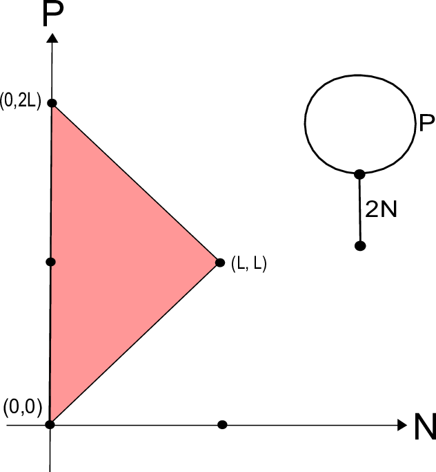

The balanced polytope corresponding to the weightings of an internal trinode has dimension It is the convex hull of and For the standard regions of this polytope with respect to appear in [M1], Figure . For this polytope is a non-normal subpolytope of the unit square, this is the reason for the condition in theorem 1.9. It was shown in [M1] that each of the standard regions of are normal, with quadratic generating relations, except for the region at the origin, the convex hull of and This polytope has one cubic relation,
| (13) |
this is why Theorem 1.9 stipulates that relations are generating by quadrics and cubics instead of just quadrics.
Next we analyze the polytope A lattice point of this polytope is given by non-negative integers which satisfy the triangle inequalities and the parity condition. The conditions defining weightings force the quantities and are forced to be even integers. We begin by subjecting this polytope to a change of coordinates.
| (14) |
| (15) |
Under this transformation, becomes the polytope on four numbers subject to the conditions,; ; . The projection of onto the plane produces a quadrilateral, shown in Figure 11 with the fibers of the projection depicted above each lattice point. The polytope has symmetry, which divides it into four isomorphic quadrants. We represent these quadrants with interlacing diagrams on numbers below. Arrows in the diagrams point from smaller entries to larger entries, in particular the polytope corresponding to an interlacing diagram with a single arrow with entries bounded by is the simplex with vertices in
Every entry at the top of a diagram is less than or equal to , and every element at the bottom is greater than or equal to
Proposition 5.3.
The quadrant is a balanced polyope.
Proof.
We establish that every element in a Minkowski sum has a balancing. Consider the interlacing diagram in the top left of the above diagram. For we form two new elements, one in and the other in by multiplying by (resp. and taking ceiling (resp. floor). Since and were arbitrary, we can repeat this process until we obtain elements in Note that this proves and therefore are normal polytopes.
Given two elements obtained from by this process, we can then form the balancing of in in the same way. By Proposition 2.9, the resulting new factorization of has weight less than or equal to the weight of the original factorization, with equality occuring exactly when the entries of are balanced with respect to each other. This implies that if a factorization of is not balanced, we may lower its weight with some pairwise balancing, and after a finite number of these moves, we obtain a balanced factorization of ∎
Remark 5.4.
The above proof can be adapted to any polytope defined by interlacing patterns. For example, this style of proof can be used to establish that the Gel’fand-Tsetlin polytope defined by a dominant weight is balanced.
Since is composed of isomorphic copies of , it follows that it is a balanced polytope as well. We now introduce a term order on the lattice points of For two lattice points, we first order by degree, then we order by the term-order. We complete this to a total term order as follows, iff or and or and or and This induces a monomial order on polynomial ring which surjects onto the semigroup algebra
Proposition 5.5.
The term order defined above induces a quadratic square-free Gröbner basis on the binomial ideal
Proof.
We sketch the proof. First, by design, any standard region of the above term order will be a sub-set of a standard region of the ordering. Note that we have shown that the standard regions of this term order are the intersections of with some integer translate of the unit cube. These are all isomorphic to polytopes with entries between and subject to the inequalities defined by some sub-interlacing diagram of the defining diagram of A selection of these are depicted below.
First we treat the polytope The semigroup defined by this polytope is generated by six lattice points, subject to one relation, It follows that has a quadratic square-free Gröbner basis with respect to the above term order.
We now consider the polytopes corresponding to proper subdiagrams. Any such diagram has no loops, so it follows that the corresponding balanced piece of can be represented, as in Proposition 1.23, as a fiber product of simplices with term orders over unit intervals. Furthermore, this fiber product can always be ordered in such a way that the resulting term order agrees with the one defined above. As a consequence of Proposition 1.23, each balanced piece of each has a quadratic, square-free Gröbner basis with respect to the term order, and it follows that has such a Gröbner basis as well. ∎
Each of the above polytopes, and come with distinguished maps to the interval given by projecting onto the weight on a non-loop edge and dividing by The polytope has three such projections, and have two, and and each have one. Each of these maps is given by forgetting coordinates off the edge, so they correspond to a coordinate projection. If a monomial is balanced then it is easy to verify that any map which forgets coordinates gives another balanced monomial. This implies that each of the edge projections above are morphisms in to This allows us to prove Propositions 1.9 and 1.10.
Proof of Propositions 1.9, 1.10.
In the first case, is a fiber product of balanced polytopes satisfying the stated conditions, therefore inherits these conditions by Propositions 1.20, 1.21.
The second case is similar, only we use Proposition 1.23 to establish that inherits a quadratic, square-free Gröbner basis. ∎

References
- [A] T. Abe, Projective normality of the moduli space of rank 2 vector bundles on a generic curve,Transactions AMS, Vol. 362 ,2010, pp. 477-490.
- [AGS] V. Alexeev, A. Gibney, and D. Swinarski, Conformal blocks divisors on from , http://arxiv.org/abs/1011.6659.
- [B] A. Beauville, Conformal Blocks, Fusion Rules, and the Verlinde formula Proceedings of the Hirzebruch 65 Conference on Algebraic Geometry, 75–96, Israel Math. Conf. Proc., 9, Bar-Ilan Univ., Ramat Gan (1996).
- [Bu] V. Buczynska, Toric models of graphs., http://arxiv.org/abs/1004.1183.
- [BW] W. Buczynska and J. Wiesniewski, On the geometry of binary symmetric models of phylogenetic trees, J. European Math. Soc. 9 (2007) 609-635.
- [E] D. Eisenbud Commutative Algebra With A View Toward Algebraic Geometry, Graduate Texts in Mathematics 150, Springer-Verlag, 1995.
- [F] N. Fakhruddin, Chern classes of conformal blocks on , 2009. arXiv:0907.0924v2 [math.AG].
- [HH] M. Hering, B. Howard, private communication.
- [Ko] T. Kohno, Conformal Field Theory and Topology, Translations of Mathematical Monographs, vol. 210, AMS, Providence, Rhode Island, (2002).
- [LS] Y. Lazlo and C. Sorger, The line bundles on the moduli of parabolic G-bundles over curves and their sections, Ann. Sci. Ecole Norm. Sup. (4) 30 (1997), 499-525.
- [M1] C. Manon, Presentations of semigroup algebras of weighted trees, J. Alg. Comb. 2010 31: 467-489.
- [M2] C. Manon The Algebra of Conformal Blocks, arXiv: 0910.0577
- [P] M. Popa, Generalized Theta Linear Series on Moduli Spaces of Vector Bundles on Curves, arXiv:0712.3192
- [St] B. Sturmfels, Gröbner bases and convex polytopes, University Lecture Series, vol. 8, American Mathematical Society, Providence, RI, 1996.
- [StX] B. Sturmfels and Z. Xu, Sagbi Bases of Cox-Nagata Rings, arXiv:0803.0892v2 [math.AG].
- [Su] S. Sullivant. Toric fiber products, J. Algebra 316 (2007), no. 2, 560–577.
- [TUY] A. Tsuchiya, K. Ueno, and Y. Yamada, Conformal field theory on universal family of stable curves with gauge symmetries, Adv. Studies in pure Math. 19 (1989) 459-566.
Christopher Manon:
Department of Mathematics,
University of California, Berkeley,
Berkeley, CA 94720-3840 USA,
August 24, 2026