Magnon decays in planar ferromagnet Spin waves Quantized spin models, including quantum spin frustration Nonmetallic ferromagnetic materials
Spontaneous magnon decays in planar ferromagnet
Abstract
We predict that spin-waves in an easy-plane ferromagnet have a finite lifetime at zero temperature due to spontaneous decays. In zero field the damping is determined by three-magnon decay processes, whereas decays in the two-particle channel dominate in a transverse magnetic field. Explicit calculations of the magnon damping are performed in the framework of the spin-wave theory for the square-lattice ferromagnet with an anisotropy parameter . In zero magnetic field the decays occur for with . We also discuss possibility of experimental observation of the predicted effect in a number of ferromagnetic insulators.
pacs
75.30.Dspacs
75.10.Jmpacs
75.50.Dd1 Introduction
Zero-point fluctuations are generally present in quantum antiferromagnets, whereas their role in ferromagnetic structures is usually considered as minor [1, 2]. Without challenging the fundamental reason behind this conclusion, we present here an example of a quantum effect specific to anisotropic ferromagnets. Namely, we predict that magnons in an easy-plane ferromagnet have a finite lifetime at zero temperature due to spontaneous three-particle decays. In contrast, excitations in a simple two-sublattice antiferromagnet remain stable at [3, 4] and acquire nonzero decay rate only above a threshold magnetic field [5, 6, 7, 8, 9, 11, 10].
The low-frequency dynamics of an isotropic ferromagnet is governed by conservation of the total spin . The ferromagnetic ground state and excited states can be classified according to , where the -axis is chosen parallel to the spontaneous magnetisation. In particular, the ground state has and every magnon carries an intrinsic quantum number . Spin conservation translates into conservation of the total number of spin waves by magnon-magnon interaction. Particle non-conserving processes, including spontaneous decays, are forbidden by symmetry for the Heisenberg ferromagnet.

In the case of an easy-plane ferromagnet the spontaneous magnetisation is orthogonal to the principal -axis, see fig. 1a. The rotation symmetry is completely broken and no value of can be assigned either to the ground-state or to low-energy excitations: spin of a spin-wave ceases to exist. Absence of conserved physical quantities other than the total momentum allows various processes that change the magnon number. Among them, spontaneous decays, fig. 1c and 1d, determine lifetime of magnetic excitations at zero temperature. The necessary condition for damping is conservation of energy in an elementary decay process. In the following we use the spin-wave theory to study spontaneous magnon decays in an easy-plane ferromagnet in the two cases: with and without transverse magnetic field. In the former case both two- (fig. 1c) and three-particle (fig. 1d) decay processes are present, whereas in the latter case only three-particle decays are compatible with the mirror symmetry .
The predicted magnon decays at may be observed in easy-plane ferromagnets such as [12, 13, 14], [15] and [16]. The second class of physical systems relevant to our work is the lattice boson models [17, 18, 19]. The equivalence between an spin-1/2 ferromagnet and a system of hard-core bosons was established a long time ago by Matsubara and Matsuda [20, 21]. Bose-Einstein condensates of cold atoms in optical lattices provide an experimental realization of such bosonic systems [22]. The analogy between field-induced transitions in quantum magnets and the Bose-Einstein condensation (BEC) of particles was explored in many experimental and theoretical studies, for review, see [23]. The main focus was so far on the critical properties of magnon BEC. The dynamical aspects of magnon condensation have started to attract attention only recently [5, 7, 6, 8, 9, 10, 24, 11]. An easy-plane ferromagnet exhibits a quantum critical point in a transverse magnetic field [21, 25], which can be mapped onto the BEC of magnons [26]. Therefore, investigation of the dynamics of a ferromagnetic model also helps to clarify universal dynamical properties of the Bose-Einstein condensates.
2 Model
In this Letter we investigate the zero-temperature dynamics of the quantum ferromagnet on a square lattice given by the nearest-neighbour Hamiltonian
| (1) |
with an easy-plane anisotropy and an arbitrary spin . The model (1) describes magnetic properties of layered ferromagnet , which has a small anisotropy and an extremely weak exchange coupling between square planes: [12, 13, 14].
In zero magnetic field the ferromagnetic moment is oriented arbitrarily in the -plane breaking the rotation symmetry. In a finite field the magnetisation tilts away from the easy-plane by an angle , see fig. 1b. The mean-field (classical) expression for the tilting angle at zero-temperature is
| (2) |
For local magnetic moments become completely aligned with the applied field and the rotation symmetry is restored. The transition at provides a simple example of the quantum critical point [21, 25, 26].
We use the spin-wave theory to calculate the damping of magnetic excitations in the model (1) at . The derivation for the anisotropic ferromagnet closely follows a similar analysis for a quantum two-sublattice antiferromagnet in external field [5, 10]. The Hamiltonian (1) is rewritten in a tilted coordinate system such that the new -axis is directed parallel to the equilibrium magnetisation. Bosonisation of spin operators is performed in the new frame using the Holstein-Primakoff transformation [1, 2]
| (3) |
. Square roots are subsequently expanded to the first order in and terms up to the fourth order in boson operators and are taken into account.
At the harmonic level the boson Hamiltonian is diagonalized by the Bogolyubov transformation
| (4) |
The bare magnon energy for is
| (5) |
with , while the Bogolyubov coefficients are given by
| (6) |
Zero-point fluctuations in the ground state are controlled by the parameter . They are gradually suppressed by the transverse magnetic field and vanish at .

The broken symmetry in an easy-plane ferromagnet is reminiscent of the breaking of the gauge symmetry in the superfluid state of a Bose gas [20, 21]. Accordingly, the energy spectrum of a quantum ferromagnet features an acoustic branch instead of the ‘normal’ ferromagnetic dispersion , see fig. 2. Direct expansion of (5) in small yields
| (7) |
where .
The excitation spectrum remains gapless up to the critical field .
The magnon velocity is positive in small fields and vanishes at
. While the critical behaviour is mostly independent of
the second subleading term in the expansion (7),
the dynamical properties crucially depend on the convexity of the
acoustic branch [27].
Considering the anisotropy/field dependence of the coefficient
we can distinguish three different regimes:
(i) for , is a convex function
of for and for all in-plane directions of the momentum;
(ii) for and , the curvature of
remains positive near the diagonal
in the Brillouin zone but becomes negative along the principal directions
;
(iii) for and , has negative curvature
at , however, there is a threshold magnetic field above which
becomes positive again:
| (8) |
A similar change in the convexity of the acoustic branch in a finite magnetic field takes place in quantum antiferromagnets [5].
In the isotropic ferromagnet () the expression for the energy of a single-magnon excitation is exact, whereas for the harmonic result (5) is only approximate. We have calculated the lowest-order Hartree-Fock correction to (5) in zero field determined by quartic magnon terms [28]. Results are shown in fig. 2 by dashed lines. The quantum correction is momentum dependent shifting in opposite directions the acoustic branch and the high-energy magnons. For and , the magnon velocity is increased by 11%, which is comparable to the 16% enhancement for the spin-1/2 square-lattice Heisenberg antiferromagnet [4]. Accordingly, the change in the curvature of the acoustic branch takes place at rather than at 1/7. For , the quantum renormalization does not exceed 3–4% for any . In the following we disregard completely the real part of the quantum correction to the spectrum of the ferromagnet and focus on the magnon damping given by .
3 Two-magnon decays
In the canted magnetic structure at , the principal nonlinear interaction is provided by the cubic term:
| (9) |
After transforming to Bogolyubov bosons one obtains two types of cubic vertices [5]. The magnon damping at is determined by the two-magnon decay vertex expressed in our case as
| (10) | |||
The decay vertex vanishes at and . In the high-field phase this is due to the spin conservation. In zero field, magnons have no well-defined spin but still preserve the odd parity under . The parity conservation forbids the two-particle decays in zero field, though the three-particle decay processes are still possible.

In the Born approximation, the magnon decay rate in the two-particle channel is given by the imaginary part of the diagram in fig. 1c:
| (11) |
Since the decay rate (11) is independent of the spin value .
Spontaneous two-particle decays are allowed if the energy conservation condition
| (12) |
is satisfied for a given magnon dispersion. For the acoustic mode (7) solutions of eq. (12) exist only for positive values of the coefficient [10, 27]. Following the preceding analysis, we conclude that the low-energy magnons in the model (1) are kinematically unstable for already in vanishingly small field. Expanding the vertex (10) in small momenta we explicitly obtain for the acoustic mode
| (13) |
Scaling is characteristic for two-dimensional models [5, 6]. The decay rate for a 3D anisotropic ferromagnet behaves similar to the phonon damping in the superfluid 4He: [27].
Away from the limit, a part of the Brillouin zone with unstable magnons can be determined numerically by solving (12) for various incoming momenta. For the decay region occupies a finite area already at and spreads out quickly over the entire Brillouin zone with increasing magnetic field. The magnon decay rate for arbitrary momenta is obtained by numerical integration of eq. (11). along two symmetry directions in the Brillouin zone is shown in fig. 3 for and several values of the transverse magnetic field. The decay rate is strongest at intermediate fields , though it remains significant up to . The decrease of as is partly compensated by a growing phase-space volume of solutions of eq. (12). Jumps and peaks in the momentum dependence of seeing in fig. 3 are respectively produced by the decay thresholds and the logarithmic singularities in the two-magnon density of states of a 2D model [29].
A finite lifetime of low-energy spin waves in an easy-plane ferromagnet in applied field was briefly discussed in [25]. Overall, physics of two-particle decays in the canted ferromagnetic state is quite similar to the field-induced magnon decays in quantum antiferromagnets [5, 7, 6, 8, 9, 10]. In particular, the asymptotic expression for (13) remains valid both in the present case and for the square-lattice Heisenberg antiferromagnet. Also, the self-consistent treatment of the decay processes beyond the Born approximation removes the 2D Van Hove singularities in [10]. Away from peaks, the decay rate is not significantly modified by higher-order processes and the Born approximation results presented in fig. 3 may serve as a guidance for future experimental tests.

4 Three-magnon decays
We now turn to zero-field magnon decays, which distinguish anisotropic ferromagnets from collinear antiferromagnets. At the two-magnon decays (10) are forbidden by symmetry. Still, for the energy conservation condition (12) can be satisfied in a certain region in the momentum space. An example of the kinematic threshold for two-particle decays is shown in fig. 4 for and . As was discussed by Harris and co-workers [3], if magnons are stable against two-particle decays in the entire Brillouin zone, then three-particle decay processes
| (14) |
are also energetically forbidden. Here, we encounter an opposite situation: conservation of energy and momentum for the two-magnon processes (12) implies that decays in the three-particle channel (14) are possible as well [30]. To our knowledge, quantum three-particle decays have not been systematically studied in the literature. Therefore, apart from specific model results we will also discuss below a few general aspects of three-particle decay processes.
The three-magnon decay region in the case of and is shown in fig. 4 by shaded area. Its boundary can be determined in a way similar to the two-particle decay threshold boundary [27, 29]. In particular, velocities of three created quasiparticles are equal to each other at the decay threshold. In fact, a stronger condition of equal momenta for the decay products holds for the model dispersion (5):
| (15) |
The three-particle decays typically occur in a larger part of the Brillouin zone, which encloses the two-magnon decay boundary.
The interaction part responsible for three-particle decays is given by
| (16) |
Derivation of the vertex function follows the same route as the preceding analysis of the cubic terms. We skip, therefore, further technical details and avoid presenting a cumbersome expression for . The magnon damping is given by the imaginary part of the diagram in fig. 1d:
| (17) |
Since , the decay rate (17) scales as representing a higher-order quantum effect compared to the two-magnon damping (11).

The momentum dependence of along the diagonal in the Brillouin zone is shown on the main panel of fig. 5 for three different values of the anisotropy parameter . Because of the spin dependence of eq. (17), we used for illustration. For other values of spin is further reduced by a factor . The decay rate behaves linearly in the vicinity of the decay threshold boundary, whereas the Van Hove singularity inside the continuum yields a nonanalytic contribution , which shows up as a shoulder-type feature on all curves in fig. 5. For both types of anomalies one finds an extra factor compared to the behaviour of the two-particle decay rate [29].
At small momenta the interaction vertex (16) exhibits a complicated non-analytic behaviour, similar to the momentum dependence of spin-wave interactions in quantum antiferromagnets [3, 31]. In particular, can have a finite limiting value depending on the order in which , and are taken to 0. Nevertheless, for the on-shell processes (14) the vertex acquires a normal hydrodynamic form [27]
| (18) |
and vanishes as . Substituting (18) into eq. (17) we obtain the power-law asymptote for the decay rate at low energies: . The derived power-law behaviour is checked on the inset of fig. 5. The deviation between the straight line and the data points at small is due to the representation of the delta-function by a finite-width Lorentzian. In the three-dimensional case the power-law exponent changes to . Both cases are included in the general expression
| (19) |
This is again to be compared with a magnon damping in the two-particle channel: [6, 29].
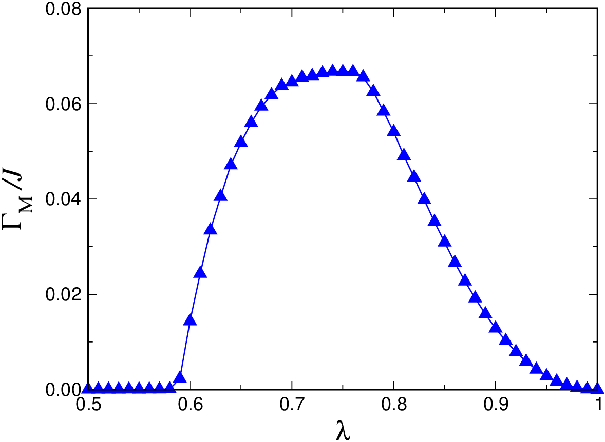
An interesting aspect of the obtained results is the dependence of on anisotropy. At small momenta the damping decreases with an increase of following the suppression of the decay vertex . In the vicinity of the Brillouin zone boundary the tendency is reversed and is primarily determined by the expanding decay region and a growing phase-space volume of the decay solutions of eq. (14). Eventually, decays disappear completely at . The details of such a non-monotonous dependence are shown in fig. 6 for the magnon damping at the M-point. Summarizing the above results we conclude that the easy-plane anisotropy in the range –0.85 is most favorable for an experimental observation of the three-particle decays.
In a finite magnetic field (fig. 1b) the decay rate is given by a sum of contributions from different decay channels. Therefore, for not too small , the magnon lifetime is dominated by two-particle decays. Still, three-magnon decay processes, being less restrictive on the value of the initial momentum, will promote decays beyond the two-particle decay region. Higher-order two-magnon processes, such as a self-energy insertion in the inner lines of the diagram in fig. 1c, can be regarded as an effective renormalization of the three-particle decay vertex and have a similar effect on the promotion of magnon decays [10]. As a result, magnons in the entire Brillouin zone acquire finite lifetimes. Note, that such a behaviour is not entirely universal. For the triangular antiferromagnet two- and three-magnon decay regions coincide and the magnon damping occurs only in a part of the Brillouin zone [29].
5 Conclusions
We have theoretically investigated zero-temperature magnon decays in an easy-plane ferromagnet with the exchange anisotropy. The phenomenon of spontaneous magnon decays depends only on symmetry (absence of spin conservation) and kinematics (curvature of the spectrum). Hence, decays should be also present in ferromagnets with the single-ion anisotropy and different lattice structures. The most significant damping is produced by two-particle decays, which are induced by a transverse magnetic field . In regard to a possible experimental observation of the predicted effects, square-lattice ferromagnet with is perhaps too isotropic to have a sizable magnon damping. Quasi-one-dimensional ferromagnet [15] has a moderate single-ion anisotropy and provides a good experimental system to test the predicted effects.
Spontaneous three-particle decays is the only damping mechanism in collinear magnetic structures. For the model case studied here the corresponding decay rate is somewhat small (). However, the significance of three-particle decays extends beyond the present model. In a collinear antiferromagnet, three-magnon decays are usually impossible due to the kinematic constraint [3]. However, sizable frustration may significantly modify the excitation energy . In particular, if an acoustic branch has an upward curvature at , then the energy conservation will allow three-particle decays. This scenario is realized in the vicinity of the quantum Lifshitz point. A typical zero-temperature transition in frustrated spin models is a second-order transition between commensurate and incommensurate antiferromagnetic structures. At the transition point, the magnon velocity vanishes at least in one direction in the momentum space producing a positive curvature of . Hence, three-particle decays are present in the commensurate state, whereas two-particle decays appear in the incommensurate phase [29].
Acknowledgements.
We acknowledge stimulating discussions with M. Mourigal and S. Raymond. We are grateful to M. Gvozdikova for help with the numerical integration and to A. Chernyshev for careful reading of the manuscript. Part of this work was performed within the Advanced Study Group Program on “Unconventional Magnetism in High Fields” at the Max-Planck Institute for the Physics of Complex Systems.References
- [1] \NameMattis D. C. \BookThe Theory of Magnetism\PublSpringer, Berlin \Year1981.
- [2] \NameMajlis N. \BookThe Quantum Theory of Magnetism \PublWorld Scientific, Singapore \Year2007.
- [3] \NameHarris A. B., Kumar D., Halperin B. I. Hohenberg P. C. \REVIEWPhys. Rev. B 31971961.
- [4] \NameManousakis \REVIEWRev. Mod. Phys. 6319911.
- [5] \NameZhitomirsky M. E. Chernyshev A. L. \REVIEWPhys. Rev. Lett. 8219994536.
- [6] \NameKreisel A., Sauli F., Hasselmann N. KopietzP. \REVIEWPhys. Rev. B 782008035127.
- [7] \NameSyljuasen O. F. \REVIEWPhys. Rev. B 782008180413(R).
- [8] \NameSyromyatnikov A. V. \REVIEWPhys. Rev. B 792009054413.
- [9] \NameLüscher A. Läuchli A. M. \REVIEWPhys. Rev. B 792009195102.
- [10] \NameMourigal M., Zhitomirsky M. E. Chernyshev A. L. \REVIEWPhys. Rev. B 822010144402.
- [11] \NameMasuda T., Kitaoka S., Takamizawa S., Metoki N., Kaneko K., Rule K. C., Kiefer K., Manaka H. Nojiri H. \REVIEWPhys. Rev. B 812010100402.
- [12] \NameHarikawa K. Ikeda H. \REVIEWJ. Phys. Soc. Jpn. 3519731328.
- [13] \NameFunahashi S., Moussa F. Steiner M. \REVIEWSolid State Commun. 181976433.
- [14] \NameBorovik-Romanov A. S., Kreines N. M., Zhotikov V. G., Laiho R. Levola T. \REVIEWJ. Phys. C 131980879.
- [15] \NameSteiner M., Kakurai K. Kjems J. K. \REVIEWZ. Physik B 531983117.
- [16] \NameRaymond S., Panarin J., Givord F., Murani A. P., Boucherle J. X. Lejay P. \REVIEWPhys. Rev. B 822010094416.
- [17] \NameScalettar R. T., Batrouni G. G., Kampf A. P. Zimanyi G. T. \REVIEWPhys. Rev. B 5119958467.
- [18] \NameMurthy G., Arovas D. Auerbach A. \REVIEWPhys. Rev. B 5519973104.
- [19] \NameBryant T. Singh R. R. P. \REVIEWPhys. Rev. B 762007064520.
- [20] \NameMatsubara T. Matsuda H. \REVIEWProg. Theor. Phys. 161956569.
- [21] \NameHalperin B. I. Hohenberg P. C. \REVIEWPhys. Rev. 1881969898.
- [22] \NamePethick S. J. Smith H. \BookBose-Einstein Condensation in Dilute Gases \PublCambridge University Press, Cambridge \Year2008.
- [23] \NameGiamarchi T., Rüegg Ch. Tchernyshyov O. \REVIEWNature Physics 42008198.
- [24] \NameZheludev A., Garlea V. O., Masuda T., Manaka H., Regnault L.-P., Ressouche E., Grenier B., Chung J.-H., Qiu Y., Habicht K., Kiefer K. Boehm M. \REVIEWPhys. Rev.B 762007054450.
- [25] \NameBaryakhtar V. G., Zhukov A. I. Yablonskii D. A. \REVIEWFiz. Tverd. Tela 211978776 [\REVIEWSov. Phys. Solid State 211979454].
- [26] \NameSyromyatnikov A. V. \REVIEWPhys. Rev. B 752007134421.
- [27] \NameLifshitz E. M. Pitaevskii L. P. \BookStatistical Physics, Part 2 \PublPergamon Press, Oxford \Year1980.
- [28] \NameOguchi T. \REVIEWPhys. Rev. 1171960117.
- [29] \NameChernyshev A. L. Zhitomirsky M. E. \REVIEWPhys. Rev. Lett. 972006207202; \REVIEWPhys. Rev. B 792008144416.
- [30] \NameMaris H. J. \REVIEWRev. Mod. Phys. 491977341.
- [31] \NameKopietz P. \REVIEWPhys. Rev. B 4119909228; \NameHasselmann N. Kopietz P. \REVIEWEurophys. Lett. 7420061067.