Density Fluctuations in the Yukawa One Component Plasma:
An accurate model for the dynamical structure factor
Abstract
Using numerical simulations, we investigate the equilibrium dynamics of a single component fluid with Yukawa interaction potential. We show that, for a wide range of densities and temperatures, the dynamics of the system are in striking agreement with a simple model of generalized hydrodynamics. Since the Yukawa potential can describe the ion-ion interactions in a plasma, our results have significant applicability for both analyzing and interpreting the results of x-ray scattering data from high power lasers and fourth generation light sources.
pacs
52.27.Gr,05.20.JjI Introduction
Recently, using high power lasers and fourth generation x-ray sources, it has become possible to create and diagnose extreme states of matter relevant to Inertial Confinement fusion (ICF) and the cores of compact astrophysical objects in the laboratory [1, 2, 3, 4, 5]. A particularly exciting development is that x-ray Thomson scattering experiments will soon be able to fully resolve time dependent ion dynamics in dense plasmas [1, 6, 7]. These ion dynamics are encoded in the wavevector and frequency dependent ion-ion structure factor (or simply dynamical structure factor), , which is the Fourier transform in space and time of the density autocorrelation function. For forthcoming experiments, an accurate model for the ion-ion structure factor is needed.
In a previous work [8], we found that the conventional hydrodynamic description (Navier-Stokes equations) reproduces well for , where and is the electronic screening length. Despite the success of the conventional hydrodynamic description at these large lengthscales (small ), a model that works well at higher (momentum transfer) is generally of greater applicability to the experiments. Fortunately, a well known framework - generalized hydrodynamics - already exists for extending the results of conventional hydrodynamics to these higher values. In this paper, we compare one of the simplest models of generalized hydrodynamics to the results of state of the art numerical simulations for . We show that the model works remarkably well for all values, i.e. the model describes both the conventional hydrodynamic limit at small values and the large behaviour (when the ions behave as a collection of free particles), along with the entire intermediate dynamics between these two regimes. Our results thus show that this simple model has significant applicability for analyzing and interpreting the results of forthcoming x-ray scattering experiments using fourth generation light sources.
This paper is structured as follows. In Sec. II, the Yukawa system - which represents interacting ions in a plasma - is introduced and details of our numerical simulations of this system are given. In Sec. III, the generalized hydrodynamics framework is summarized, along with the Gaussian approximation for the memory function that leads to a simple model for . This model is then shown to very accurately reproduce the results of our numerical simulations in Sec. IV. Also in this Section, we briefly discuss the applicability of our results to x-ray scattering experiments (Sec. IV.5), before offering our conclusions in Sec. V.
II Numerical Simulations
We consider a plasma consisting of one species of ions of charge and mass at temperature and density . Because the ions are much more massive than the electrons, on the time scale of the ion dynamics of interest here, electrons instantaneously screen the ion-ion Coulomb interactions and their degrees of freedom are not treated explicitly. We take the Yukawa potential,
to represent the screened interaction between ions. The electronic screening length [9, 10, 3] reduces to either the Debye-Huckel law or the Thomas-Fermi distance in the limiting cases of classical and degenerate electron fluid respectively [1].
This single component system is known to be fully characterised by two dimensionless parameters only [11]. These are: (i) the coupling strength
where is the average inter-particle distance, and (ii) the screening parameter
In our MD simulations, we compute the dynamical structure factor, , of the Yukawa system for various values (,,,,,) at , thereby spanning a range of thermodynamic conditions 11 1 We have also performed some simulations at other values; the model presented in Sec. III.1 works very well for these other values, but here we present results for only.. In our simulations, the dynamics of particles mutually interacting through the Yukawa potential are resolved using the Verlet algorithm in periodic boundary conditions [12]. In all cases, we include the Ewald summation in our force calculation - this is essential for small values - using the particle-particle-particle-mesh (PPPM) method [13]. The rms error of our force calculation is . We find that obtaining accurate MD data for requires averaging the results of a large number of simulations to improve statistics. This computational demand has made a thorough study such as ours impractical before now. For example, compared with the study of Hansen for the OCP system [14] - which, even after more than years remains the primary source of MD data for quantitative studies of that system [15] - we use 20 times as many particles, a smaller timestep by a factor of , and simulation times times as large. Our timestep , where is the ion plasma frequency, ensures excellent energy conservation (). Moreover, we find that the long length of our simulations, for every and value, is of paramount importance: while it is possible to capture the essential features of with simulations significantly shorter than this, producing a spectrum that is of sufficient accuracy to draw conclusions about the validity of various models requires simulations of approximately this length (we note that our data for changes negligibly by increasing the simulation time beyond ). In particular, these long simulation times are essential for computing accurately the decay time of collective modes at small values (i.e. the width of the ion-acoustic peak in ).
In a previous work [8], we presented MD results for of the Yukawa system at small values; the MD data showed that the conventional hydrodynamic description works well in describing the dynamics providing , where . The new MD results presented here are for a significantly larger range of values; in this paper we are interested in finding a model that reproduces the MD data for all values.
III Model
III.1 Model for
In the hydrodynamic regime, the wavevector and frequency dependent ion-ion structure factor can be written
| (1) |
where is the static ion-ion structure factor. Equation (1) is the result obtained from the linearised Navier Stokes equation [16, 12]. Here is the (isothermal) sound speed and is the kinematic viscosity. Equation (1) clearly has considerable similarity to the expression that underlies the model we will consider in this article
| (2) |
Equation (2) is a well known and exact representation of that can be formally derived from microscopic theory [17]. The similarity to Eq. (1) is no coincidence: Eq. (2) represents a generalized hydrodynamics in which both equilibrium properties and transport coefficients are replaced by suitably defined wavevector dependent quantities. In Eq. (2), defines a generalised isothermal sound speed that, in the hydrodynamic limit of , reduces to the conventional isothermal sound speed , where is the isothermal compressibility of the system and that of an ideal gas. The quantities and are respectively the real and imaginary parts of the Laplace transform of the memory function : in the analogy between Eqs. (1) and (2), the memory function plays the role of a generalized viscosity.
The model we present here amounts to using the Gaussian ansatz for the memory function,
| (3) |
where is given in terms of the frequency moments of
| (4) |
Explicit expressions for , and are given in the Appendix. Here , appearing in Eq. (3), is a wavevector dependent relaxation time. According to Eq. (3), the real and imaginary parts of the Laplace transform of the memory function are given by, respectively [18, 14],
| (5) |
and
| (6) |
where the Dawson function [19].
The quality of the Gaussian model has been previously identified for the Lennard-Jones fluid [18, 20] and by Hansen et al. in a pioneering study of the One Component Plasma (OCP) [14]; it has also been applied to experimental data for weakly coupled plasma produced by arc jets [21]. However, because of the difficulty of conducting highly accurate numerical simulations at the time of the previous investigations, a detailed, conclusive comparison of the model in Eq. (2) with the results of Molecular Dynamics (MD) simulations was not possible for those systems. Here, with the aid of modern computing facilities, we have conducted accurate, large scale MD simulations for across a wide range of thermodynamic conditions. We find that the Gaussian model matches the MD data for the Yukawa system very well for all thermodynamic conditions we have examined in our simulations.
III.2 Physical discussion of model for
The structure factor in the hydrodynamic regime, as given in Eq. (1), can be derived from the longitudinal component of the linearized Navier Stokes equation,
| (7) |
where is the longitudinal current density and is the pressure. Similarly, Eq. (2) can be derived from a generalized version of Eq. (7) (see [18] for more details),
| (8) |
where is the number density. This generalization is motivated in the following way. At small length scales, the validity of the conventional hydrodynamic description can be expected to break down. Specifically, in the Navier Stokes description of Eq. (7), both the pressure term and viscosity term are local in space and time. The generalization in Eq. (8) includes the non-local behavior that is essential at small length scales in two ways. Firstly, it is assumed that a change in pressure at a position should not be determined completely by density fluctuations at the same position but also by density fluctuations at neighbouring positions. This means that the pressure gradient due to a density gradient is non-local (hence the functional derivative appearing in Eq. (8)). Secondly, the viscosity is made to be non-local in space and time to model the viscoelastic effects in a real liquid. The memory function that models these viscoelastic effects describes the delayed response of the longitudinal part of the stress tensor to a change in the rate of shear [18]. In Eq. (3), this response is modeled by a single relaxation time . The requirement that the model reproduces the result obtained from the Navier-Stokes equations in the hydrodynamic limit gives a relation between the long wavelength behavior of this relaxation time and the kinematic viscosity [18],
| (9) |
where , with and the shear and bulk viscosities respectively.
The generalization included in Eq. (8) leads to the expression in Eq. (2) for the dynamical structure factor (see e.g. [18]). All that remains is to specify the memory function. As discussed in Sec. III.1, here we choose a Gaussian memory function, as this is the simplest model that previous studies have suggested gives a good description of the dynamics of classical fluids. We find that this choice yields a model of the dynamical structure factor that matches the MD data for the Yukawa system remarkably well.
IV Results and Analysis
The Gaussian memory function model given in Eqs. (2), (5) and (6) requires values for , and for each . Since all three of these parameters are in general unknown, we have fitted them to the MD spectrum of using the least squares method. That is to say, for each value for which we have computed with MD (these are the values compatible with the periodic boundary conditions in our simulations), we fit the model to the MD spectrum of . When this is done, the model reproduces the MD data very accurately for all and values; in Sec. IV.1 we show that this is the case for small, intermediate and large values (see also [22]).
The three parameter fit is the correct way to compare the Gaussian memory function model to the MD spectrum of . This is true despite the fact that two of the parameters, and , can in principle be obtained by computing (or equivalently the radial distribution function [12]) with MD and using the formulae given in the Appendix A. When obtained from MD in this way, these two parameters are subject to numerical incertainty. Therefore, one would expect that constraining and - and therefore fitting the model to the MD spectrum using only a single parameter [14, 18, 21] - would result in poorer fits and larger errors. In Fig 1, we show that in general this is indeed the case.
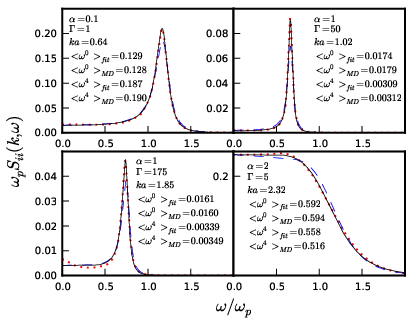
The validity of the three parameter fit can be confirmed by comparing the fitted values of the two parameters and to their values when instead computed with MD as described above. As shown in Figs. 2 and 3, the parameters and obtained from the fit to the MD spectrum of agree very well (within ) with those computed from the MD and . This is only the case because the model works so well. For example, as shown in Fig. 3, if an exponential rather than Gaussian memory function is used (this is known as the viscoelastic model and is discussed in Sec. IV.3), the numerical values obtained for by fitting the model with three parameters do not agree well with those computed from the MD and . In the remainder of the paper, we present only the results for the Gaussian memory function model with three fitting parameters; the one parameter fits are irrelevant as their comparison with the MD data for is not indicative of the quality of the model.


IV.1 Comparison between model and MD simulations
We find that in general the Gaussian memory function model reproduces the MD data very well for all of the (,,,,,) and (, and ) values we have considered, at all values (our simulations are for ). Extended figures of our complete MD results are available as supplementary material [22]; here, in Figs. 4 - 6, we show only a selection of these complete results at small, intermediate, and large respectively.


At small values (Fig. 4), for all and , the MD data shows a clear ion-acoustic (or Brillouin) peak that represents a damped sound wave in the plasma. In this regime, the model extends the conventional hydrodynamic description to finite values. Specifically, the generalised sound speed along with the imaginary part of correct for the fact that the position of the peak does not vary linearly with as in the hydrodynamic description [8], and the real part of corrects for the width.
At intermediate values (Fig. 5), the model gives a surprisingly accurate account of both the width and position of the ion acoustic peak. This is particularly true for . For higher values, the MD data does in some cases show additional structure which the model cannot recreate. In particular, for , a two peak structure is visible for and a three peak structure for (e.g. Fig. 5, top left). The small peak just below for is of particular interest - it does not appear to have been seen or commented upon in previous MD calculations. We note that this peak is distinct from the higher harmonic peaks reported in [23]. In fact, at only, we do see signs of a second harmonic peak, at a frequency close to . We have neglected this harmonic peak in our analysis, since we find it to be more than than 3 orders of magnitude smaller than the main features in the spectrum of , in good agreement with [23]. On the other hand, the peak shown in Fig. 5 (top left) is of the same order of magnitude as the main features of . We believe that this peak is due to microscopic ‘caging’ effects (e.g. [12, 17]). That is, at these lengthscales, the relatively high frequency oscillations of individual particles in the cages produced by their neighbors are imprinted on . We note that although the model does not fully capture the additional structure in the MD data for these conditions, on average it does give a good account of the overall shape of the spectrum.
At large values (Fig. 6), reduces to a single peak at . In this regime, the model reproduces the MD data very accurately in all cases. As increases, should tend to its ideal gas limit , which is independent of [14, 12],
| (10) |
As shown in Fig. 7, at constant , as increases converges more slowly towards . Indeed, at the highest value we have considered in our MD simulations (), the MD result only compares well to its ideal gas limit for (see Fig. 7). We note that the discrepancy between and its ideal gas limit can more readily be seen by looking at the MD data for the static structure factor ; the ideal gas limit will only be approximated at values for which (since ).

In any case, as shown in Fig. 6, the Gaussian model compares very well to the MD data at our highest value of , regardless of whether or not this value is sufficiently large for to be close to its ideal gas limit.
IV.2 Hydrodynamic limit
In previous investigations (e.g. [18]), Eq. (9) was used to infer the kinematic viscosity from the long wavelength behavior of the relaxation time appearing in the memory function. For the Yukawa system, in principle this could be used to determine the shear viscosity (the bulk viscosity is in general negligible in comparison with the shear viscosity for the Yukawa system [24]). However, due to the inaccuracy inherent in measuring the width of the (very narrow) ion acoustic peak obtained from the MD simulations at small values, we find that this method is of little practical use compared to other approaches to determining the viscosity. These alternative approaches include utilizing the Green-Kubo relation for the shear stress autocorrelation function [25], non-equilibrium molecular dynamics methods [26], and computation of the transverse current autocorrelation function [27].
Along with the generalized viscosity, as discussed in Sec. III.1, in the hydrodynamic limit the generalized sound speed reduces to the conventional (isothermal) sound speed . The small behaviour of the generalized viscosity and sound speed thus ensure that using the Gaussian ansatz for the memory function in Eq. (2) gives a result that is compatible with the result obtained from the linearised Navier Stokes equations [12] when thermal fluctuations are neglected. To be clear, Eq. (2) is an entirely general (i.e. exact) representation of . The effective neglect of thermal fluctuations is made by assuming the ansatz in Eq. (3). That is to say, in the case of the Gaussian ansatz it is instructive to think of the memory function as a sort of generalized viscosity. There is no term in the memory function that represents the effects of temperature fluctuations i.e. a generalized (or indeed non-generalized) thermal conductivity.
It is straightforward to modify Eq. (3) so that the result from the Navier Stokes equations including temperature fluctuations is recovered in the hydrodynamic limit (see e.g. [16, 18]). The simplest extension involves maintaining a generalized sound speed and viscosity, and adding the (non-generalized) thermal conductivity contribution obtained from conventional hydrodynamics (the Navier-Stokes equations) as an additional term in the memory function. In a more involved scheme, this additional contribution can also be generalized [20, 16].
For the Yukawa system with the and values we have considered here, including in the memory function the effects of thermal fluctuations is unnecessary. This is because the ratio of specific heats, , is very close to , as indicated by the absence of a Rayleigh peak at for small in the MD data (Fig. 4), as well as previous equation of state calculations [28]. The only cases in which this peak - which represents a diffusive thermal mode - is not negligible is for the more weakly coupled () systems at (see Fig. 4, bottom left). As expected, the model does not capture this peak in the MD data.
The fact that for the Yukawa system with the and values considered here is certainly a reason why the Gaussian memory function works so well. Indeed, the ansatz in Eq. (3) would not be expected to work as well when the ratio of specific heats is noticeably different from unity [17]; this includes the Yukawa system for .
IV.3 Comparison with viscoelastic model
Given the excellent agreement between the MD data and the Gaussian memory function model, we have not found it necessary to undertake an exhaustive comparison with the numerous other forms of memory function proposed in the literature [16]. However, here we briefly comment on another widely studied and used ansatz for the memory function
| (11) |
When combined with Eq. (2), Eq. (11) - which represents the simplest assumption that can be made about the time dependence of the memory function - is known as the viscoelastic model [17].
As indicated in Fig. 8 and discussed in detail elsewhere [17, 20, 18], the viscoelastic model cannot capture the shape of across a large range of values. While the model works well at small (indeed, for the viscoelastic model the results of isothermal hydrodynamics are again recovered, with a relation between the relaxation time and the kinematic viscosity similar to Eq. (9)), the model tends to predict rather more structure in than is evident in the MD data (Fig. 8). Clearly then the Gaussian memory function is vastly superior to the exponential one.

IV.4 Discussion of the relaxation time

Fig. 9 shows the relaxation time as determined from the fit of the Gaussian model to the MD spectrum of for . As shown in Fig. 9, we find that as increases, decreases. This agrees qualitatively with e.g. the behavior of the relaxation time determined for the Lennard-Jones fluid in previous investigations [18, 29]. One certainly expects that at decreasing wavevectors, the relaxation time should increase: as , the memory function should decay fast enough to guarantee the validity of the Markovian approximation, which itself is related to the fulfillment of the conservation laws [17].
In our investigation, we find that at the very smallest values accessible to our simulations (i.e. below , which is the minimum value shown in Fig. 9), the numerical value of is difficult to extract from the MD spectrum reliably, and therefore it is not possible to examine the exact behavior of the relaxation time. That is to say, the fitted value of at these small values does not connect smoothly to the values at higher values; this is because the spectrum consists of a very sharp peak, for which it is difficult to accurately determine the parameters in the Gaussian model (see also Sec. IV.2).
Physically, the relaxation time controls the specific collective behavior of the system: for times the system responds ‘elastically’ (i.e. like a ‘frozen’ solid-like system), wheras for times the viscous mechanisms set in and reveal the inherent dynamic disorder [17]. Therefore, the decrease in as increases corresponds physically to the fact that at increasingly short lengthscales, viscous behavior is observed at increasingly short timescales.
IV.5 Applicability to x-ray scattering experiments
In a previous work [8], it was shown that the conventional hydrodynamic description (i.e. Eq. (1)) is valid providing , where . This means that experiments designed to measure [1] at values below can in principle be used to determine transport (e.g. viscosity) and thermodynamic properties (e.g. compressibility) of dense plasmas.
At values larger than , our results show that the Gaussian memory function model extends the conventional hydrodynamic description very satisfactorily. Thus experiments for measure the generalized quantities appearing in the memory function model of Eq. (2).
Present x-ray scattering experiments are also concerned with diagnosing the density and temperature of dense plasmas [1]. For this task theoretical models for how depends on density and temperature are required. In the Yukawa system, the density and temperature are encoded in and . Thus here we briefly look qualitatively at how changes with and : this gives an indication of how the experimental scattering cross section should vary with density and temperature. We restrict ourselves to the region of values for which shows a clear ion-acoustic peak, since then its description reduces to the position, width and height of this peak.

Fig. 10 shows how the position, width and height of the ion-acoustic peak as extracted from our MD simulations vary with reduced wavenumber for a number of and values. As shown in the top left panel of Fig. 10, the dependence on of the ion-acoustic peak position is almost identical for a large range of values (i.e. ). The peak width and height do show more discernible differences for these values. At smaller values (, and ), the differences in the position, width and height of the peak are greater.
At constant (right panels of Fig. 10), the peak position is rather different for , and . In this case, the width and height are more similar, particularly for and .
We expect that a given experiment will be able to determine peak position, width and height at a specific wavenumber (determined by the scattering angle and x-ray wavelength [1]). The extraction of and values could then be done by using these experimental results in conjunction with a set of three plots as shown in Fig. 10.
Of course, our discussion in this section assumes that a real physical plasma at a certain density, temperature and (average) ionization state can be described by the Yukawa system. While in principle this mapping could be attempted for any given values of these plasma parameters, our main interest at present concerns the dense (approximately solid density), liquid-like plasmas at temperatures of that can be created in high power laser experiments [1]. Recently, a method for mapping the physical parameters of these states to the Yukawa model (i.e. determination of and ) has been suggested [30]. Therefore, we expect that the results we have obtained for the Yukawa system are certainly relevant for future experiments that will measure ion dynamics of these extreme states of matter.
V Concluding Comments
The Gaussian memory function model is an extremely good representation of the dynamical structure factor of the Yukawa system for a wide range of thermodynamic conditions. The model very accurately reproduces the spectrum of from MD in terms of just 3 parameters and, as such, it is a useful way of accurately condensing or representing such data. This conclusion was only possible because of the highly accurate MD data presented in this paper. The model can be used by fitting either a single parameter or three parameters to the spectrum of at a particular value; in the latter case, the small numerical inaccuracies that arise in the MD simulations can be accounted for.
Why exactly this form of memory function should work so well is an interesting question that certainly merits further investigation. Other memory function models, such as the viscoelastic model (an exponential memory function) do not compare well to the MD data for a wide range of values. It is possible that the reason a faster decaying (compared to exponential) Gaussian works well is related to the chaotic nature of classical systems - this is reflected in the relatively short ‘memory’ of the system.
Since the Yukawa system can describe ion-ion interactions in a plasma, our results are applicable to future x-ray scattering experiments that will attempt to measure ion dynamics in dense plasmas [7]. In particular, our MD results for the position, width and height of the ion-acoustic peak could be used to infer the thermodynamic conditions of dense plasmas.
VI Acknowledgements
This work was supported by the John Fell Fund at the University of Oxford and by EPSRC grant no. EP/G007187/1. The work of J.D. was performed for the U.S. Department of Energy by Los Alamos National Laboratory under Contract No. DE-AC52-06NA25396. J.D. and J.P.M. gratefully acknowledge the support of the US Department of Energy through the LANL/LDRD Program for this work.
*
Appendix A Frequency moments of
The wavevector dependent quantities,
| (12) |
and
| (13) |
are given in terms of the frequency moments of , defined as
| (14) |
The zeroth moment of gives the static structure factor
| (15) |
The second moment is
| (16) |
where is the reduced wavevector ( is the Wigner-Seitz radius) and is the (ion) plasma frequency. The fourth moment is (see [17], Eq. (1.137))
| (17) |
Here , the Einstein frequency is given by
| (18) |
and
| (19) |
Eqs. 17 - 19 give an exact expression for the fourth moment for the Yukawa one component plasma.
References
- [1] S.H. Glenzer and R. Redmer, Rev. Mod. Phys. 81, 1625 (2009).
- [2] B.A. Remington et al., Rev. Mod. Phys. 78, 755 (2006).
- [3] E. Garcia Saiz et al., Nat. Phys. 4, 940 (2008).
- [4] B. Nagler et al., Nat. Phys. 5, 693 (2009).
- [5] A.L. Kritcher et al., Science 322, 69 (2008).
- [6] A. Pelka et al., Phys. Rev. Lett. 105, 265701 (2010).
- [7] G. Gregori and D.O. Gericke, Phys. Plasmas 16, 056306 (2009).
- [8] J.P. Mithen, J. Daligault and G. Gregori, Phys. Rev. E 83, 015401(R) (2011).
- [9] K. Wünsch, J. Vorberger and D.O. Gericke, Phys. Rev. E 79, 010201 (2009).
- [10] D. Kremp, M. Schlanges and W.D. Kraeft, Quantum Statistics of Nonideal Plasmas (Springer-Verlag, Berlin, 2005).
- [11] Z. Donkó, G.J. Kalman and P Hartmann, J. Phys.: Condens. Matter 20, 413101 (2008).
- [12] J.P. Hansen and I.R. McDonald, Theory of Simple Liquids (third edition) (Academic Press, 2006).
- [13] R. Hockney and J. Eastwood, Computer Simulations Using Particles (McGraw-Hill, New York, 1981).
- [14] J.P. Hansen, I.R. McDonald and E.L. Pollock, Phys. Rev. A 11, 1025 (1975).
- [15] Yu.V. Arkhipov, A. Askaruly, D. Ballester, A.E. Davletov, I.M. Tkachenko and G. Zwicknagel Phys. Rev. E 81, 026402 (2010).
- [16] J.P. Boon and S. Yip, Molecular Hydrodynamics (Dover, 1980).
- [17] U. Balucani and M. Zoppi, Dynamics of the Liquid State (OUP, 2002).
- [18] N.K. Ailawadi, A. Rahman and R. Zwanzig, Phys. Rev. A 4, 1616 (1971).
- [19] A method for implementing the Dawson function can be found in W.H. Press et al., Numerical Recipes in C (second edition) (Cambridge, 1992).
- [20] I.M. de Schepper et. al. Phys. Rev. A 38, 271 (1988).
- [21] G. Gregori, U. Kortshagen, J. Heberlein and E. Pfender Phys. Rev. E 65, 046411 (2002).
- [22] See EPAPS Document No. [number will be inserted by publisher] for these extended figures. The numerical data for these figures can be obtained by contacting the corresponding author.
- [23] P. Hartmann et al., J. Phys. A: Math. Theor. 42, 214040 (2009).
- [24] G. Salin and J. Caillol, Phys. Plasmas 10, 1220 (2003).
- [25] T. Saigo and S. Hamaguchi, Phys. Plasmas 9, 1210 (2002);
- [26] Z. Donkó and B. Nyíri, Phys. Plasmas 7, 45 (2000).
- [27] Z. Donkó, J. Goree and P. Hartmann Phys. Rev. E 81, 056404 (2010).
- [28] S. Hamaguchi, R.T. Farouki and D.H.E. Dubin, J. Chem. Phys. 105, 7641 (1996) ; S. Hamaguchi, R.T. Farouki and D.H.E. Dubin Phys. Rev. E 56, 4671 (1997).
- [29] D. Levesque, L. Verlet and J. Kürkijarvi, Phys. Rev. A 7, 1690 (1973).
- [30] M.S. Murillo, Phys. Rev. E 81 036403 (2010).