In the last years it has become clear that multiple parton interactions play an important role in hadron-hadron collisions at high energies [1, 2, 3, 4, 5, 6, 7, 8]. As a first step these chains are modelled as a collection of single noninteracting chains (Fig.1).

Each chain follows the usual partonic DGLAP evolution, i.e. the ladders are in color singlet states, and the momentum transfer across the ladder is set equal to zero. Disregarding final state radiation and working in leading order only, the final state produced by $k$ such chains consists of $N=n_{1}+n_{2}+...+n_{k}$ partons, and the cross section, $d\sigma\sim|T_{2\to N}|^{2}d\Omega_{N}$, is described by a sum of squares, without any interference terms.

The theory of multiparton (higher twist) evolution has been outlined in [9]. To leading order, the evolution is described by the sum over the pairwise interactions between two $t$-channel partons, and the evolution kernels are given by the nonforward DGLAP splitting functions. Of particular importance is the small-$x$ region where powers of $\ln 1/x$ may compensate (and even overcome) the higher twist suppression. In this region, the dominant contributions are given by gluon ladders, and their evolution in $\ln 1/x$ is described by the BKP equations [10]. In leading order this evolution is, again, described by the sum over parwise interactions between $t$-channel gluons. The evolution kernels are given by the nonforward BFKL-kernels. At small $x$, the leading logarithmic approximations of the two approaches - higher twist evolution in momentum scale or small-$x$ evolution in $\ln 1/x$ - coincide in the so-called ’double logarithmic approximation’ which samples powers of $(\alpha_{s}\ln 1/x\ln p^{2})$.

For both evolution schemes the t-channel multiparton state is in a color singlet state and, as far as the total cross section is concerned, the total momentum transfer is set equal to zero. However, any subsystem consisting of two $t$-channel gluons, in general, will have nonzero color quantum number and nonzero momentum transfer. Therefore, describing the evolution of a $t$-channel state consisting of, say, $2n$ gluons as the evolution of $n$ noninteracting color singlet ladders with zero momentum transfer represents an approximation whose validity deserves further investigation.

In this note we study, as a first correction beyond the approximation of noninteracting ladders, a particular type of ’interactions’ between two ladders which we illustrate in Fig.2:

Starting at the proton at the bottom of Fig.2, we first have two noninteracting color singlet ladders (denoted by the pairs of $t$-channel gluons $(14)$ and $(23)$). At rapidity $Y$ we allow for a ’recombination’ of $t$-channel gluons: from now on we have the two color singlet pairs $(13)$ and $(24)$. In the following we will denote his transition by ’recombination vertex’. It introduces a correlation between the two ladders. However, it is important to note that, in the double log approximation, this kind of interaction between the two ladders still belongs to the leading logarithmic approximation: for each momentum integral we have a factor $(\alpha_{s}\ln p^{2}\ln 1/x)$. It is this kind interaction between the two ladders which we will study in the following, staying within the double logarithmic approximation of gluon ladders. Particular attention will be given to the possibility that this recombination of two chains takes place in the perturbative region, i.e. in the region of large transverse momenta.

Recently an important potential application of such recombination effects has been suggested. In their attempt to explain the ridge effect reported by the CMS group at the LHC [11], it has been suggested [12] that the observed long range rapidity correlation and azimuthal correlation can be explained, within the Color Glass Condensate framework, by a two-chain recombination which will be discussed in this paper.

We begin with the double logarithmic approximation of the two-chain configurations shown in Figs.1 and 2: we search for regions of integration where each closed momentum loop gives two logarithms, one in the transverse momentum and one in rapidity. We restrict ourselves to gluon ladders which, at small $x$, are known to give the largest contributions. We parametrize our momenta as

$$k=xp_{A}+yp_{B}+\mbox{\boldmath$k$}$$

(1)

where $p_{A}$, $p_{B}$ are the large momenta of the incoming protons $A$ and $B$, resp., the momentum fractions $x$, $y$ range between $0$ and $1$, and $k$ denotes the two dimensional transverse momentum. In the double logarithmic approximation, the BFKL kernel and the splitting function $P_{gg}$ lead to the same answer (Fig.3): we can either start from the small-$x$ limit which is described by the BFKL equation and then take the limit of strongly different momentum scales; alternatively, we can begin with the collinear limit where the DGLAP equations apply and then take the limit of small $x$. For our purposes it will turn out that the approach based upon the BFKL equation is more suitable: it is the region where the logarithms in $1/x$ are slightly larger than the transverse momentum logarithms where the recombination effects become important.

In the region of strongly ordered transverse momenta the color singlet BFKL kernel is approximated by

$$g^{2}\left(-\mbox{\boldmath$q$}^{2}+\frac{\mbox{\boldmath$k$}^{2}(\mbox{\boldmath$q$}-\mbox{\boldmath$k$})^{2}+{\mbox{\boldmath$k$}^{\prime}}^{2}(\mbox{\boldmath$q$}-\mbox{\boldmath$k$}^{\prime})^{2}}{(\mbox{\boldmath$k$}-\mbox{\boldmath$k$}^{\prime})^{2}}\right)\approx 2g^{2}\mbox{\boldmath$k$}^{\prime}(\mbox{\boldmath$k$}^{\prime}-\mbox{\boldmath$q$})$$

(2)

This approximation will be used in the following.

We begin with the two noninteracting ladders shown in Fig.1. Our main focus is on the integration over the loop momentum $q$, and we consider a single cell with momentum $\mbox{\boldmath$k$}^{\prime}$ inside one of the ladders below the produced pairs of jets. This cell is illustrated in Fig.3. Using (2) for the upper rung (and the corresponding expression for the lower rung), together with the gluon propagators for the vertical lines, one sees that the integration over the transverse momentum $\mbox{\boldmath$k$}^{\prime}$ is logarithmic only if $k^{\prime}\gg q$, i.e. $q$ defines the momentum scale $Q_{0}$ where the $\mbox{\boldmath$k$}^{2}$ evolution along the ladders starts. On the other hand, the range of the integration over the momentum transfer along the ladders is determined by the size of the interaction region and by the correlation length of the initial gluons of the two ladders inside the proton: we denote this effective radius by $\tilde{R}$, and put $Q_{0}^{2}=1/{\tilde{R}}^{2}$. As a result, the cross section for the production of two pairs of gluon jets (cf. Fig.1) will be of the form:

$$\frac{d\sigma}{dY_{1}dY_{2}d^{2}\mbox{\boldmath$p$}_{1}d^{2}\mbox{\boldmath$p$}_{2}}\sim\frac{1}{{\tilde{R}}^{2}}\frac{1}{(\mbox{\boldmath$p$}_{1}^{2})^{2}}\frac{1}{(\mbox{\boldmath$p$}_{2}^{2})^{2}}f(x_{1},\mbox{\boldmath$p$}_{1}^{2})f(y_{1},\mbox{\boldmath$p$}_{1}^{2})f(x_{2},\mbox{\boldmath$p$}_{2}^{2})f(y_{2},\mbox{\boldmath$p$}_{2}^{2})$$

(3)

where $f(x,\mbox{\boldmath$p$}^{2})=xg(x,\mbox{\boldmath$p$}^{2})$ denotes the gluon density with initial momentum scale $Q_{0}^{2}$, the factor $1/{\tilde{R}}^{2}$ results from the integration over the loop momentum $q$, and the momentum factors $1/(\mbox{\boldmath$p$}_{1}^{2}\mbox{\boldmath$p$}_{2}^{2})^{2}$ represent the two production vertices of the pairs of gluon jets (evaluated in the double logarithmic approximation).

As an important feature of (3) we mention that, as long as interactions between different parton chains are not taken into account, the momentum transfer along a ladder is of the order of the initial momentum scale of the (multi)parton distribution.

We now turn to the main topic of this paper, a study of the two recombinations shown in Fig.2. We begin with the recombination vertex below the produced jets; the kinematics are illustrated in Fig.4,. Above the recombination, the two ladders formed by the lines (13) and (24) are in the color singlet configuration; below the color singlet ladders are formed out of (14) and (23). As a result, each color recombination is accompanied by the color suppression factor

$$\frac{1}{N_{c}^{2}-1}$$

(4)

In order to have, for the momentum loops below the lower two rungs (connecting $(14)$ and $(23)$), logarithmic momentum integrals, we need

$$|\mbox{\boldmath$k$}^{\prime}_{1}|,|\mbox{\boldmath$k$}^{\prime}_{2}|\gg|\mbox{\boldmath$l$}|.$$

(5)

Similarly, in order to find logarithmic momentum integrals above the upper two rungs (connecting (13) and (24)), we need

$$|\mbox{\boldmath$k$}_{1}|,|\mbox{\boldmath$k$}_{2}|\gg|\mbox{\boldmath$q$}|,$$

(6)

Finally, inside the $k$ loop of Fig.4. we need

$$|\mbox{\boldmath$k$}_{1}|,|\mbox{\boldmath$k$}_{2}|\gg|\mbox{\boldmath$k$}|\gg|\mbox{\boldmath$k$}^{\prime}_{1}|,|\mbox{\boldmath$k$}^{\prime}_{2}|,\,\,\,|\mbox{\boldmath$k$}|\gg|\mbox{\boldmath$l$}|,\,\,\,|\mbox{\boldmath$k$}_{1}|,|\mbox{\boldmath$k$}_{2}|\gg|\mbox{\boldmath$k$}^{\prime}_{1}|,|\mbox{\boldmath$k$}^{\prime}_{2}|.$$

(7)

Using, for the upper two rungs, the approximations following from (2), and combining them with the propagators for the vertical gluon lines, we obtain:

$$(2N_{c}g^{2})^{2}\int\frac{d^{2}k}{(2\pi)^{3}}\int\frac{d^{2}q}{(2\pi)^{3}}\frac{2\mbox{\boldmath$k$}(\mbox{\boldmath$k$}-\mbox{\boldmath$q$})}{\mbox{\boldmath$k$}^{2}(\mbox{\boldmath$q$}-\mbox{\boldmath$k$})^{2}}\frac{2\mbox{\boldmath$k$}(\mbox{\boldmath$k$}-\mbox{\boldmath$q$})}{\mbox{\boldmath$k$}^{2}(\mbox{\boldmath$q$}-\mbox{\boldmath$k$})^{2}}$$

(8)

In order to obtain a logarithmic integrals of $k$, we identify two regions of $k$ and $q$: either $|\mbox{\boldmath$q$}|\gg|\mbox{\boldmath$k$}$ or $|\mbox{\boldmath$q$}|\gg|\mbox{\boldmath$q$}-\mbox{\boldmath$k$}|$. For each of the two cases, after averaging over the azimuthal angle, we arrive at the integrals

$$2g^{4}\int\frac{d^{2}q}{(2\pi)^{3}}\frac{1}{\mbox{\boldmath$q$}^{2}}\int^{q^{2}}\frac{d^{2}k}{(2\pi)^{3}}\frac{1}{\mbox{\boldmath$k$}^{2}}$$

(9)

which gives the desired logarithmic integral in $k$ (or ($\mbox{\boldmath$q$}-\mbox{\boldmath$k$}$)).

For the two ladders below the recombination we derive, from the condition (7) and from the second integral in (9), that the upper cutoff is given by $q^{2}$. The lower cutoff is obtained by applying the discussion of section 2.1: the loop momentum $l$ appears only inside the initial condition of the lower proton $B$, and it is restricted by the effective scale $Q_{0}^{2}$ The condition (6) implies that the momentum $q$ also defines the lower momentum cutoff for the ladders above the recombination vertex.

In order to find the full dependence on $q^{2}$, we need to consider the full diagram in Fig.2 ¹¹ 1 Otherwise the momentum $q$ will run through the blob corresponding to the proton initial conditions and, like the momentum $l$, it will be restricted by a low scale $Q_{0}$.. The recombination vertex above the produced pairs of jets is analysed in the same way as the lower one. This leads to an expression similar to (9), i.e. the complete dependence in $q$ is of the form:

$$\int\frac{d^{2}q}{(\mbox{\boldmath$q$}^{2})^{2}},$$

(10)

The integral in $q$ is dominated by small values. Since the momentum $q$ defines the upper momentum cutoff, both for the two ladders below the lower recombination vertex and for the two ladders above the upper recombination vertex, we conclude that the infrared divergence of the $q$-integration destroys the ladders above and below the recombination vertices. The recombination vertices, therefore, are absorbed into the nonperturbative initial conditions. As far as the perturbative part is concerned, we are back to the two noninteracting chains of section 2.1.

The situation changes if logarithms in rapidity become more important than those in transverse momentum, i.e. within the BFKL approach we move towards small $x$. In Fig.2, we replace the rungs by BFKL Green’s functions. Re-drawing the diagram in an more suitable way, we arrive at Fig.5:

Let us first reformulate the result which we have just obtained in the double logarithmic approxmation. We have shown that, in order to find inside the BFKL Green’s function the maximal number of transverse logarithms, the momentm transfer across the Green’s function has to be smaller than the transverse momenta of the two gluons entering the Green’ function at the low-momentum side. In Fig.5. this says that $l$ and $\mbox{\boldmath$l$}^{\prime}$ have to be small, while for the $q$-loop we found the integral $\int dq^{2}/q^{4}$ which favors small values, too.

In order to see how the appearance of large rapidity intervals changes this situation, let us use the following integral representation for the forward BFKL-Green’s function:

$$G(k,k^{\prime};Y-Y^{\prime})=\int\frac{d\omega}{2\pi i}e^{\omega(Y-Y^{\prime})}\int\frac{d\nu}{2\pi i}\left(\frac{k^{2}}{{k^{\prime}}^{2}}\right)^{\mu}\frac{1}{\omega-\chi(\mu,0)},$$

(11)

where $\mu=i\nu+\frac{1}{2}$, the integration contours in $\mu$ and $\omega$ run parallel to the imaginay axis, $\chi(\mu,n)$ is the BFKL eigenvalue function, and we have averaged over the azimuthal angles of $k$, $\mbox{\boldmath$k$}^{\prime}$. Furthermore, we have kept only the leading term of the conformal spin, $n=0$. From this representation one easily deduces the dependence upon $Y-Y^{\prime}$ and $\ln\frac{k^{2}}{{k^{\prime}}^{2}}$: after the integration over $\omega$ the saddle point analysis of the remaining $\mu$ -integral shows that, for large $\ln\frac{k^{2}}{{k^{\prime}}^{2}}$, the dominant contributions come from $\mu=i\nu+\frac{1}{2}\approx 0$ and $\omega={\cal O}(1)$, whereas for large $Y-Y^{\prime}$, one finds $\mu\approx\frac{1}{2}$ and small $\omega=\omega_{BFKL}=\frac{4N_{c}\ln 2\alpha_{s}}{\pi}$. This observation has important consequences. Let us denote the rapidities of the two recombinations by $Y^{\prime}$ and $Y$, resp.. Beginning with the BFKL amplitudes near the produced jets, large rapidity intervals $Y^{\prime}-Y_{1}$, $Y_{1}-Y$, $Y^{\prime}-Y_{2}$, $Y_{2}-Y$ increase the corresponding anomalous dimensions and hence favor larger values of the central loop momentum, $q$. To see this im more detail, we insert the integral representations for all the BFKL Green’ function in Fig.5. We arrive at

$$\frac{d\sigma}{dY_{1}dY_{2}d^{2}\mbox{\boldmath$p$}_{1}d^{2}\mbox{\boldmath$p$}_{2}}\sim\frac{1}{R^{2}_{c}}\frac{1}{R_{c}^{2}}\frac{1}{(\mbox{\boldmath$p$}_{1}^{2})^{2}}\frac{1}{(\mbox{\boldmath$p$}_{2}^{2})^{2}}\int\frac{d\mu^{\prime}}{2\pi i}\int\frac{d\mu}{2\pi i}\int\frac{d\mu^{\prime}_{1}}{2\pi i}\int\frac{d\mu_{1}}{2\pi i}\int\frac{d\mu^{\prime}_{2}}{2\pi i}\int\frac{d\mu_{2}}{2\pi i}\cdot$$

$$\int dY\int dY^{\prime}\int\frac{d^{2}q}{q^{4}}\Big[\left(\frac{\mbox{\boldmath$q$}^{2}}{Q_{0}^{2}}\right)^{\mu^{\prime}}e^{(Y_{tot}-Y^{\prime})\chi(\mu^{\prime})}\Big]^{2}\cdot$$

$$\Big[\left(\frac{\mbox{\boldmath$p$}_{1}^{2}}{\mbox{\boldmath$q$}^{2}}\right)^{\mu_{1}^{\prime}}e^{(Y^{\prime}-Y_{1})\chi(\mu_{1}^{\prime})}\Big]\Big[\left(\frac{\mbox{\boldmath$p$}_{1}^{2}}{\mbox{\boldmath$q$}^{2}}\right)^{\mu_{1}}e^{(Y_{1}-Y)\chi(\mu_{1})}\Big]\Big[\left(\frac{\mbox{\boldmath$p$}_{2}^{2}}{\mbox{\boldmath$q$}^{2}}\right)^{\mu_{2}^{\prime}}e^{(Y^{\prime}-Y_{2})\chi(\mu_{2}^{\prime})}\Big]\Big[\left(\frac{\mbox{\boldmath$p$}_{2}^{2}}{\mbox{\boldmath$q$}^{2}}\right)^{\mu_{2}}e^{(Y_{2}-Y)\chi(\mu_{2})}\Big]\cdot$$

$$\cdot\Big[\left(\frac{\mbox{\boldmath$q$}^{2}}{Q_{0}^{2}}\right)^{\mu}e^{Y\chi(\mu)}\Big]^{2}$$

(12)

Here we have introduced another length scale, $R_{c}^{2}$: it results from the additional integrals (as compared to eq.(3)) $d^{2}\mbox{\boldmath$l$}$ and $d^{2}\mbox{\boldmath$l$}^{\prime}$, which are restricted by the proton radius and by the correlation between the two chains inside the proton. As long as all BFKL amplitudes are in DGLAP regime, i.e. they are dominated by the logarithms in the transverse momenta, all $\mu$ variables are small, and we are in the situation which we have described above: the $q$ integral is dominated by small values, and the transverse momentum logarithms inside those four BFKL amplitudes which are close to the protons are destroyed. If, however, the rapidity intervals become large and the BFKL amplitudes are in the small-$x$ region, $\mu$ values are close to $\frac{1}{2}$. As a result, in (12) the overall power of $\mbox{\boldmath$q$}^{2}$ may increase and the dominance of the small-$\bf q^{2}$ region disappears. One easily sees that large rapidity intervals near the protons, $Y_{tot}-Y^{\prime}$ and $Y$, tend to make $\mu$ and $\mu^{\prime}$ large and thus help to increase the overall power of $q^{2}$.

Let us see in more detail how this balance works. Defining in (12) the phase function

$$\Phi(\mu����,\mu^{\prime}_{1},\mu_{1},\mu^{\prime}_{2},\mu_{2},\mu)=2\left((Y_{tot}-Y^{\prime})\chi(\mu^{\prime})+\mu^{\prime}\ln\frac{q^{2}}{Q_{0}^{2}}\right)+$$

	$\displaystyle+\left((Y^{\prime}-Y_{1})\chi(\mu^{\prime}_{1})+\mu^{\prime}_{1}\ln\frac{p_{1}^{2}}{q^{2}}\right)+\left((Y_{1}-Y)\chi(\mu_{1})+\mu_{1}\ln\frac{p_{1}^{2}}{q^{2}}\right)$
	$\displaystyle+\left((Y^{\prime}-Y_{2})\chi(\mu^{\prime}_{2})+\mu^{\prime}_{1}\ln\frac{p_{2}^{2}}{q^{2}}\right)+\left((Y_{2}-Y)\chi(\mu_{2})+\mu_{1}\ln\frac{p_{2}^{2}}{q^{2}}\right)$
	$\displaystyle+2\left(Y\chi(\mu)+\mu\ln\frac{q^{2}}{Q_{0}^{2}}\right),$		(13)

the saddle points are determined from the conditions:

$$0=\frac{\partial\Phi}{\partial\mu}=2\chi^{\prime}(\mu_{s})Y+2\ln\frac{q^{2}}{Q_{0}^{2}},$$

(14)

and

$$0=\frac{\partial\Phi}{\partial\mu_{1}}=\chi^{\prime}(\mu_{1,s})(Y_{1}-Y)+\ln\frac{p_{1}^{2}}{q^{2}},$$

(15)

which lead to

$$\chi^{\prime}(\mu_{s})=-\frac{\ln\frac{q^{2}}{Q_{0}^{2}}}{Y}$$

(16)

and

$$\chi^{\prime}(\mu_{1,s})=-\frac{\ln\frac{p_{1}^{2}}{q^{2}}}{Y_{1}-Y}$$

(17)

Similar equations are obtained for the other $\mu$ variables.

For a systematic analysis one first determines, for fixed $Y$, $Y^{\prime}$ and $q^{2}$, the stationary points of the $\mu$ variables and then finds the dominant values of the rapidities $Y$, $Y^{\prime}$ and of the momentum scale $\ln q^{2}$. As we have said before, if in (16) the evolution in rapidity dominates over that in momentum scale, the rhs becomes small. Since $\chi^{\prime}(\mu)$ vanishes at $\mu=\frac{1}{2}$, we have

$$\mu_{s}\approx\frac{1}{2}-\frac{1}{\chi^{\prime\prime}(\frac{1}{2})}\frac{\ln\frac{q^{2}}{Q_{0}^{2}}}{Y}.$$

(18)

On the other hand, if in (17) the interval in momentum evolution is larger than in rapidity, the rhs is large when $\mu$ is close to zero:

$$\mu_{1,s}\approx\sqrt{a\frac{Y_{1}-Y}{\ln\frac{p_{1}^{2}}{q^{2}}}}$$

(19)

with $a=\frac{N_{c}\alpha_{s}}{\pi}$ and $\chi^{\prime\prime}(\frac{1}{2})=a28\zeta(3)$ (here $\zeta(3)\approx 1.202$ denotes the Riemann zeta function).

The results can be illustrated in terms of evolution paths in Fig.6. There is an infinite number of paths in the $\ln k^{2}$-$y$ plane which connect the protons with the produced jets with rapidity $Y_{1}$, $Y_{2}$ and momenta $\mbox{\boldmath$p$}_{1}^{2}$, $\mbox{\boldmath$p$}_{2}^{2}$. The saddle point analysis determines the most probable path. Two examples are shown in Fig.6.

Let us now consider a few special cases. For simplicity, we start with the symmetric choice $Y_{1}=Y_{2}$ and $p_{1}^{2}=p_{2}^{2}=p^{2}$. In order to get a large $q^{2}$ we search for the situation where $\mu>\mu_{i}$ and $\mu^{\prime}>\mu^{\prime}_{i}$. We insert the saddle point values (18), (19) into (13), and first look for the extrema with respect to $Y$ and $Y^{\prime}$, that is for the saddle point of the expression

$$A_{lower}=e^{\sqrt{4a(Y_{1}-Y)\ln(p^{2}_{1}/q^{2})}}e^{2Y\chi(\mu_{s})}e^{\sqrt{4a(Y_{2}-Y)\ln(p^{2}_{2}/q^{2})}}$$

(20)

which belongs to the lower part of Fig.5. To get (20) we have used the value of $\mu_{s}$ in (18) and neglected a weak dependence of $\mu_{s}\sim 1/2$ on $Y$ coming from (18). Thus the typical value of $Y$ is

$$Y=Y_{s}=Y_{1}-a\frac{\ln^{2}(p^{2}/q^{2})}{\chi^{2}(\mu_{s})},$$

(21)

leading to

$$A_{lower}\sim\exp\left(\frac{2a}{\chi(\mu_{s})}\left[2\ln^{3/2}(p^{2}/q^{2})-\ln^{2}(p^{2}/q^{2})\right]+2\chi(\mu_{s})Y_{1}\right)\,.$$

(22)

An analogous expression is obtained for the upper part of the amplitude in Fig.5, $A_{up}$. Assuming that the total avaliable rapidity interval $Y_{tot}$ and the sub-rapidities $Y_{1},\ Y_{2}$ are so large that the saddle point position $\mu_{s}$ (18) is close to 1/2, i.e. $28\zeta(3)aY_{1}>>\ln(q^{2}/Q^{2}_{0})$. We put $\mu_{s}=0.5$ in (20), (22), and we see that in (12) the integral over $q^{2}$ takes the form

$$\int\frac{d\ln q^{2}}{q^{2}}\exp\left(\frac{1}{\ln 2}\left[2\ln^{3/2}(p^{2}/q^{2})-\ln^{2}(p^{2}/q^{2})\right]\right).$$

(23)

Here we have used the LO BFKL ratio $a/\chi(\mu_{s})=a/\chi(0.5)=1/4\ln 2$. The integral (23) has its saddle point at

$$q^{2}\sim p^{2}\exp(-z^{2})$$

(24)

with $z=3/4+\sqrt{9/16+0.5\ln 2}\simeq 1.7$; $\exp(-z^{2})\simeq 0.055$. The corresponding value of $\mu_{1,s}\simeq z/4\ln 2\sim 0.6$ is not small enough to justify the approximate estimate (19). We therefore conclude that the competition between the $Y$ and $q^{2}$ dependence leads to a rapidity saddle point (21) somewhere inside the avaliable interval $(Y_{1},0)$, which in its turn leads to a rather large $\mu_{i,s}$ violating the initial inequality $\mu_{i}<\mu$.

In general we can say that the ordering $\mu_{i,s}<\mu_{s}$ leads to the opposite ordering of the intercepts, $\chi(\mu_{s})<\chi(\mu_{i,s})$. Therefore, in (12) the dominant contribution to the $Y$ integral comes from the region of small $Y$ where the recombination vertex is close to the initial proton and far from the production vertex of the dijets. For a small $Y$ value the anomalous dimension $\mu$ cannot be large, and the essential $q^{2}$ values are small as well. This means that we are back to the situation of non-interacting ladders, illustrated in Fig.6a.

Next we turn to the opposite case $\mu_{i}>\mu$ which corresponds to $\chi(\mu_{i})<\chi(\mu)$. Now the dominant $Y$-value is large and close to the rapidity of high $E_{T}$ dijets $Y_{1}$. However, now the whole anomalous dimension in the $q^{2}$ behaviour $2(\mu+\mu^{\prime})-\mu_{1}-\mu^{\prime}_{1}-\mu_{2}-\mu^{\prime}_{2}<0$ is negative, and the $q^{2}$ integral is dominated by a low $q^{2}$-value.

The most interesting possibility is to put the recombination vertices just as close as possible to the high $E_{T}$ dijet production matrix elements. In this case there is no BFKL or DGLAP evolution in the intervals between the produced pairs of jets and the recombination vertices. That is, in the centre of Fig.5, we simply delete the four ’BFKL blobs’ nearest to the produced jet pairs. Correspondingly, in (12) we eliminate the third line, togather with the integrations over $\mu_{1},\mu_{2},\mu^{\prime}_{1},\mu^{\prime}_{2}$. The rapidities $Y,Y^{\prime}$ are close to $Y_{i}$, and the $q^{2}$ integral takes the form

$$\int\frac{d\ln q^{2}}{q^{2}}q^{4(\mu_{s}+\mu^{\prime}_{s})}\ ,$$

(25)

where the saddle point values, $\mu_{s}$ and $\mu^{\prime}_{s}$, follow from the condition (14):

$$0=\chi^{\prime}(\mu_{s})Y+\ln\frac{q^{2}}{Q_{0}^{2}}$$

(26)

and

$$0=\chi^{\prime}(\mu^{\prime}_{s})(Y_{tot}-Y^{\prime})+\ln\frac{q^{2}}{Q_{0}^{2}}\,.$$

(27)

Their values are taken from (18):

$$\mu_{s}\approx\frac{1}{2}-\frac{1}{\chi^{\prime\prime}(\frac{1}{2})}\frac{\ln\frac{q^{2}}{Q_{0}^{2}}}{Y}\,,$$

(28)

i.e. the integral over $q^{2}$ receives its main contribution from $q^{2}$ close to $\min\{p_{1}^{2},p_{2}^{2}\}$  ²² 2 In the region of $q>p_{i}$ the momentum $q$ will destroy the matrix element of high $E_{T,i}$ dijet production replacing in (12) the factor $1/p^{4}_{i}$ by $1/q^{4}$. This situation belongs to the evolution path shown in Fig.6b.

Let us finally consider a more realistic situation with $Y_{1}=Y_{2}$ but $p_{2}<p_{1}$. Recall that the true argument of the BFKL amplitude is not rapidity but the momentum fraction $x$, that is actually we have to take $Y=\ln(1/x)$. When $p_{1}>>p_{2}$ for the same rapidities $Y_{1}=Y_{2}$ we get in the right ladder the momentum fraction $x_{2}<<x_{1}$. In other words, in this configuration we may put, in Fig.5, the recombination vertex just into the cell nearest to the left dijet. But then there will be a large $\ln x$ (and may be $\ln q^{2}$) interval for the evolution of the right ladders (between the dijets on the rhs and the two recombination vertices. In other words in Fig.5. we delete only the two ’BFKL blobs’ on the lhs below and above the dijet production. Assuming that, in (12), the total rapidity interval $Y_{tot}$ is very large, we may perform first the rapidity integral

$$\int dY\exp[-Y(\chi(\mu_{2})-2\chi(\mu))]=\frac{1}{\chi(\mu_{2})-2\chi(\mu)}$$

(29)

where for the BFKL blobs on the lhs we have set $\chi(\mu_{1})=0$, and for $\mu$ we put its asymptotic value $\mu=1/2$. Now we close the countor of the $\mu_{2}$ integration around the pole $\chi(\mu_{2})-2\chi(\mu)=0$: this leads to $\mu_{2}\simeq 0.18$. The same result is obtained for $\mu^{\prime}_{2}$. Finally, the $q^{2}$ integral takes the form

$$\int^{p^{2}_{2}}d\ln q^{2}q^{2(1-\mu_{2}-\mu^{\prime}_{2})},$$

(30)

and the major contribution comes from the domain close to upper limit $q^{2}\sim p^{2}_{2}$.

A closer look reveals still another detail. In the region of interest, for example in a 14 TeV $pp$-collision at the LHC, we observe in the central region the dijet with $p_{1}\sim 20GeV$, corresponding to $x\sim 2p_{1}/\sqrt{s}\sim 0.003$. For such $x$-values, the anomalous dimension observed at HERA is not so large. For $x<0.01$ the behaviour of the structure function $F_{2}(x,q^{2})$ can be parametrized as

$$F_{2}=c(q^{2})x^{\lambda}$$

(31)

with $c\simeq const(q^{2})$ and $\lambda=0.048\pm 0.004$ [13]. This means that effective anomalous dimension $\mu_{eff}=\lambda\ln(1/x)\sim 0.28$ for $x=3\cdot 10^{-3}$. This value is still large enough to provide the convergence of the $q^{2}$ integral (25) in the large $q^{2}$ domain for the case considered above where both recombination vertices are jsut near the dijet production cell. However it is not evident that the parametrization (31) reflects the behaviour of a single ladder. At not large $q^{2}$ the experimentally measured $F_{2}$ already includes some absorptive effects which reduce the growth of $F_{2}$ with $x$ decreasing and thus leads to a lower value of $\lambda$ in comparison with a single ladder contribution. In other words the true value of $\mu_{eff}$ which corresponds to a single ladder may be even larger, pushing the characteristic values of $q^{2}$ closer to the (lower) hard scale $p^{2}_{2}$.

So far we have discussed the effect of two recombinations inside a two-chain contribution: one recombination on esch side of the produced jet pairs. Let us first comment on the case where we have no second recombination vertex above the jet pairs: as far as only one recombination vertex is concerned, the integration over $q$ is logarithmic. However, $q$ runs also through both upper ladders and defines the low momentum scale $Q_{0}^{2}$ where the evolution starts: a large value of $q$ therefore kills the evolution in the upper ladders, whereas a low value prevents the evolution in the lower ladders. Therefore, a single recombination vertex is suppressed.

Next a comment on the color suppression factor (4). This suppression applies to the case when, as illustrated in Fig.2, there is evolution above and below the recombination vertex. As we have discussed before, in a preferred situation we have little or no evolution between the recombination vertices and the dijet production vertices. In this case there is no need to reconnect, between the two recombination vertices, the four t-channel gluon lines to color singlet pairs. As result, the color suppression becomes much weaker..

Next we consider the case of more than two chains, say three chains with three produced pairs of jets.. In this case a pair of two recombination vertices can be attributed to any pair of chains, i.e. we have three possibilities. Similarly, for $n$ chains we have $\frac{n(n-1)}{2}$ possiblities: these counting factors can easily overcome the color suppression factor in (4). As an example, for $n=4$, the overall counting factor is already $3/4$, and it exceeds unity for $n\geq 5$.

Finally, we mention another important possibility, related to final states with rapidity gaps. Besides the recombination illustrated in Fig.2 there exists another configuration to which our discussion applies. We show this in Fig.7:

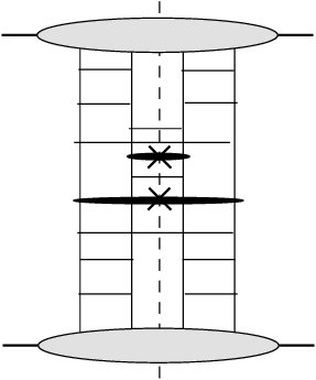
Applying our previous discussion, in particular the evolution paths illustrated in Fig.6, we conclude that the momentum scale at the upper end of the lower rapidity gap, $q^{2}$, will be above $Q_{0}^{2}$ but not too close to the jet momenta $p_{1}^{2}=p_{2}^{2}$: this allows for ’semihard’ diffraction and is in qualitative agreement with inclusive diffraction seen at HERA.

We have studied the possibility of interactions (’recombinations’) between two evolution chains, which describe double parton scattering corrections in high energy hadron collisions. We show that, thanks to large anomalous dimensions of the parton distributions in the low-$x$ region, such an interaction may occur at small distances within the pertubative domain, provided we consider two recombination vertices (which describe the chain-chain interaction) placed relatively close to the ’hard’ matrix elements.

In our double leading log analysis of gluon ladder diagrams we find a competition between ’collinear’ logarithms ($\ln\mbox{\boldmath$p$}^{2}$) and ’energy’ logarithms ($\ln(1/x)$). Depending on the ratio between these logarithms, the major contribution to integrals over the rapidity of the two recombination vertices, $Y$ and $Y^{\prime}$, comes either from the region near the protons (Fig.6a) or from the region close to the jet production vertices (Fig.6b), i.e. these integrals have no saddle point somewhere in centre of the avaliable interval. The first case (Fig.6a) corresponds to two independent ladders which do not communicate with each other and are described by ’double DGLAP’ evolution equations. More interesting is the second possibility (Fig.6b) where the recombination vertices are close to the hard matrix elements and thus are entirely in the perturbative region. These configurations may lead to nontrivial correlations between the secondaries produced in ’double parton scattering’ processes. We note that, in Fig.6b, the rapidities and transverse momenta of the partons inside the recombination vertices need not be very close to the ’hard’ matrix element: in a more or less realistic situation the convergence of the integrals in rapidity ($Y$ and $Y^{\prime}$) and transverse momentm ($q$) are rather slow, since they are driven by numerically small powers of $1/x$ and $q^{2}$. Therefore the particles coming from the recombination vertices may still be separated from those produced via the ’hard’ subprocess by relatively large intervals in rapidity ($\sim$ few units) and in the logarithms of transverse momenta.

The interactions between different ladders discussed in this paper also allow for semihard diffractive final states (Fig.7).

In the case of multiple parton interactions with a larger number of evolution chains the suppression of chain-chain interactions caused by the colour factor $1/(N^{2}_{c}-1)$ may be compensated by the combinatorical factor. For $n$ chains we have $n(n-1)/2$ possibilities. According to naive ’eikonal model’ estimates the mean number of chains in proton-proton collision at the LHC is $<n>\sim 5$. Therefore the expected probability of multi-chain recombinations is not small and may lead both to a noticeable correlation between the secondaries in inclusive processes and to ’semihard’ diffraction final states.

All results of this paper are based upon the double logarithmic approximation (with fixed $\alpha_{s}$). We consider this as a first step towards a more accurate analysis. Within the small-$x$ approach it is possible to go beyond the double logarithmic approximation and to reach single logarithmic accuracy (leading $\ln 1/x$). Also, a more detailed numerical analysis will be needed in order to obtain a more reliable estimate of the importance of the recombination corrections addressed in this paper. Both tasks will be topics of future work.

We finally mention an important consequence of our result. In contrast to non-interacting multiparton chains which often are modelled within the eikonal approximation, corrections due to the recombination of ladder diagrams no longer fit into the eikonal picture. This raises the question of the AGK cutting rules which provide a crucial theoretical constraint of multiparton corrections. An investigation of this problem is quite important.

Acknowledgements:
The work by MGR was supported by the grant RFBR 11-02-00120a and by the Federeal Program of the Russian State RSGSS-65751.2010.2.

References

- [1] D. Treleani, Phys. Rev. D 76 (2007) 076006 [arXiv:0708.2603 [hep-ph]].
- [2] E. L. Berger, C. B. Jackson and G. Shaughnessy, Phys. Rev. D 81 (2010) 014014 [arXiv:0911.5348 [hep-ph]].
- [3] J. R. Gaunt and W. J. Stirling, JHEP 1003 (2010) 005 [arXiv:0910.4347 [hep-ph]].
- [4] J. R. Gaunt, C. H. Kom, A. Kulesza and W. J. Stirling, Eur. Phys. J. C 69 (2010) 53 [arXiv:1003.3953 [hep-ph]].
- [5] M. Strikman and W. Vogelsang, Phys. Rev. D 83 (2011) 034029 [arXiv:1009.6123 [hep-ph]].
- [6] M. Diehl and A. Schafer, Phys. Lett. B 698 (2011) 389 [arXiv:1102.3081 [hep-ph]].
- [7] C. Flensburg, G. Gustafson, L. Lonnblad and A. Ster, arXiv:1103.4320 [hep-ph].
- [8] M. G. Ryskin and A. M. Snigirev, arXiv:1103.3495 [hep-ph].
- [9] A. P. Bukhvostov, G. V. Frolov, L. N. Lipatov and E. A. Kuraev, Nucl. Phys. B 258 (1985) 601.
- [10]
J. Bartels,
Nucl. Phys. B175 (1980) 365.
J. Kwiecinski, M. Praszalowicz, Phys. Lett. B94 (1980) 413.
T. Jaroszewicz, Acta Phys. Polon. B11 (1980) 965. - [11] V. Khachatryan et al. [CMS Collaboration], JHEP 1009 (2010) 091. [arXiv:1009.4122 [hep-ex]].
- [12] A. Dumitru, K. Dusling, F. Gelis, J. Jalilian-Marian, T. Lappi, R. Venugopalan, Phys. Lett. B697 (2011) 21-25. [arXiv:1009.5295 [hep-ph]].
- [13] C. Adloff et al. [ H1 collaboration ], Phys. Lett. B520 (2001) 183.