DNA Circuits Based on Isothermal Constrained Loop Extension DNA Amplification

The ICLEDA amplification method designed in patent [8] is to some extend a combination of RCA and SDA amplification. We refer to this patent for more technical information.

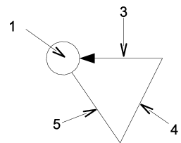
The mechanism is represented on Fig. 1(a). The loop complex is a circular molecule composed of two parts: the amplifiable fragment (2) and the loop link (1). The arrow represents the 3’ end of the amplifiable fragment. We represent this molecule schematically as on Fig. 1(b). For the sake of commodity we split the amplifiable fragment in 3 parts (3,4,5 on the picture) corresponding to the 3’ end, middle and 5’ end of the amplifiable fragment.

The amplification mix contains primers (101) which hybridize to the 3’ part of the amplifiable fragment (3). They can be further extended by DNA polymerase (102) present in the mix, see Fig. 2(a). The loop link (1) length is small compared to the length of the DNA fragment: typically 1 to 5 nm. It can be a simple chemical link joining the extremities of the DNA fragment, or a biochemical link between biotin moieties attached to the extremities of the DNA fragment via a streptavidin protein. The DNA fragment is also short in regards to the stiffness of double stranded DNA. In conditions where the biochemical replication reactions can take place, double stranded DNA molecules shorter than 300 – 500 nucleotides are too stiff for their extremities to come into close proximity. In other words, a circular DNA molecule shorter than 300 nucleotides cannot exist in full double stranded form, but is found as stretches of double stranded portions separated by single stranded portions. This is true also for the loop complexes used in ICLEDA. At some point the complex will be composed from a single stranded DNA having $n$ nucleotides from the 5’ end of the amplifiable fragment, a double-stranded DNA corresponding to the 3’ part of the amplifiable fragment, the extended primer and the linking loop of special length.

Since the two extremities of the amplifiable fragment are linked to each other this gives a geometric constraint for the loop. In order to continue the reaction either the single strand part should be extended to the maximum or the double stranded part should open at the opposite extremity. At some level of tension the energetic preference will be to continue the extension of the primer by DNA polymerase, while the opposite end will detach by Brownian motion. So, at the same time the double stranded fragment will be opened at 5’ part and one nucleotide will be added by DNA polymerase. However it should be noted that the number of nucleotides on the double stranded part remains unchanged, due to the geometric constraints of the loop.

Since no more nucleotides are bound at the 3’ end of the amplifiable fragment (3) at some point it becomes accessible for a hybridization with a new primer, see Fig. 2(b). The extension is blocked when it reaches the end on the amplifiable fragment (105) because of the presence of non-natural nucleotides in the link, see Fig. 2(c).

Fig. 3 shows a loop complex (1) which has three attached primers being in different stages of the duplication. The first primer (101a) is paired to the 3’ part of the amplifiable fragment (3) and is ready to be extended. The second primer (101b) is in the process of the extension and it is paired by its 3’ end to the central part (4) of the amplifiable fragment where its extension continues, while its 5’ part is a single stranded DNA. The third primer (101c) reached the end and is not extended anymore, but it is still paired by its 3’ end to the 5’ end (5) of the amplifiable fragment. The progression of the extension is blocked by the loop link (1), while its 5’ part is progressively detached from the amplifiable fragment by the progression of the extension of the second primer. Besides its role in the amplification process, the link also enables the possibility of attaching the loop complex to a surface without hindering the replication mechanism.

Now we remark that if in the mix a fragment of a single stranded DNA that matches the 3’ part of the amplifiable fragment is present, then it can stick to the amplifiable fragment as shown on Fig. 4(a). We call such a strand a trigger. When a trigger is attached to the loop complex, no amplification can be done. A trigger can be detached from the loop complex by an activator that matches by its 3’ end a part of the trigger strand as shown on Fig. 4(b). Once bound to the trigger the activator can be extended by DNA polymerase and this will release the trigger, so the loop complex will be able to start the amplification process.

As the main process described in the previous subsection deals with molecules, we shall represent them as words over the four-letter alphabet. However, we shall not represent individual nucleotides. We shall rather consider the places where reactions may occur. Consequently, we shall divide the words in several places, the sensitive ones and the neutral ones. If $A$ is a molecule or a part of it, we denote by $A^{\prime}$ its complement in the Watson-Crick complementarity rule. Note that $A^{\prime}$ is also written in the opposite order of its letters with respect to $A$. Molecules are oriented and we denote by the symbol $\diamond$ the head (3’ end) of the molecule, which implies the reading order from left to right for $\diamond A$ and from right to left for $A^{\prime}\diamond$.

We consider that if $A$ and $A^{\prime}$ are both present and if the configurations of the DNA strings to which they belong allow it, they bind each other. Consider that $A$ occurs in a molecule $M$. We write this $M=uAv$ with $u$ or $v$ possibly not present: we then say that $u$ or $v$ is empty. Consider that $A^{\prime}$ occurs in a molecule $M^{\prime}$. We similarly denote this by $M^{\prime}=xA^{\prime}y$. We assume that $A$ no more occurs neither in $u$ nor in $v$ and that, similarly $A^{\prime}$ no more occurs neither in $x$ nor in $y$. We also assume that $A$ and $A^{\prime}$ do not interact with neither of the molecules $u$, $v$, $x$ and $y$ and that these molecules also do no interact with each other. We express this by saying that $u$, $v$, $x$ and $y$ are neutral parts of the molecules to which they belong. This allows us to focus only on $A$ and $A^{\prime}$ which are called the sensitive parts of the molecules $M$ and $M^{\prime}$. We shall mark this difference between sensitive and neutral parts of molecules in the notation: sensitive parts will be denoted by capital letters and neutral parts will be denoted by lower case ones.

When the molecules $\diamond M$ and $N\diamond$ are both present, assuming that $\diamond M$ contains the active part $A$ and that $N\diamond$ contains $A^{\prime}$, we denote this by an additive notation: $\diamond M~\bigoplus~N\diamond$. Now, if we replace $\diamond M$ and $N\diamond$ by their expressions in terms of $A$ and $A^{\prime}$, we get $\diamond uAv~\bigoplus~yA^{\prime}x\diamond$ and we now know that as a result we obtain a complex as $A$ and $A^{\prime}$ get bound to each other. We write the complex as $\diamond uAv\otimes yA^{\prime}x\diamond$. Hence the corresponding rule can be written as follows:

As an example, we cannot write

unless $A=wB^{\prime}t$ or $B=rA^{\prime}s$, we remember the reader that lower case letters denote neutral parts. To avoid unneeded repetition of rules we shall always use the rule in its explicit form (1),considering that in (2), we have neither $A=wB^{\prime}t$, nor $B=rA^{\prime}s$.

We assume that the operation $\textstyle\bigoplus$ is commutative and associative, which corresponds to the fact that $\textstyle\bigoplus$ models a situation in which the components are independent and may freely combine or not and in all possible combinations.

The loop complex can be formalized as follows: $\nabla F^{\prime}uR^{\prime}$ where $u$ is the neutral part and $F^{\prime}$ with $R^{\prime}$ are the sensitive ones, corresponding to the parts 4,3,5 on Fig. 1(b). A trigger can be formalized as $\diamond wX^{\prime}Fz$, where $w$ and $z$ are the neutral parts and $X^{\prime}$, $F$ are the sensitive ones.

The working of the loop complex can be formalized as:

Now, if there is a trigger, we have:

We also have two rules for the trigger which occurs in formula (4):

It can be noted that the formalism allows to explain why we obtain this rule. Indeed, it might be argued that as $F^{\prime}$ and $F$ should also bind together, we could have the backward reaction:

The reason why we have not this reaction is that as $A^{\prime}$ is more visible for $A$ that $F$ is for $F^{\prime}$, $A$ attaches to the trigger which, as a result, lead to its freeing from the complex.

In what follows, to simplify the notations, we introduce the following convention: we represent the triggers $Ax\diamond$ and $zF^{\prime}Ax\diamond$ as $\mathcal{A}$. This allows us to melt the formulas (5) and (6) in a single one,namely:

We can see this higher priority of $\mathcal{A}$ in the formalism. Remember that if we wish to read the words in the order given by a run other the molecule from its head to its tail, we have to read the word from the diamond to the opposite end. Define the apartness of a sensitive molecule $X$ with respect to a molecule $M$ as the number of sensitive parts of $M$ between the diamond of $M$ and the position of $X$. Denote it by $apart(X,M)$. We can now define the apartness of $X$ with respect to $M$ and $N$, denoted by $apart(X,M,N)$, where $X$ is contained in $M$ and $X^{\prime}$ is contained in $N$, as the expression $apart(X,M)+apart(X^{\prime},N)$. Now, we can see that $apart(\mathcal{A},\hbox{$\nabla F^{\prime}uR^{\prime}\otimes\diamond tA^{\prime}Fw$},\mathcal{A})=0$ whatever the realization of $\mathcal{A}$: as $Ax\diamond$ or $zF^{\prime}Ax\diamond$. Now we have that $apart(F,\hbox{$\nabla F^{\prime}uR^{\prime}\otimes\diamond tA^{\prime}Fw$},\mathcal{A})=1$, also whatever the realization of $\mathcal{A}$. As the apartness of $\mathcal{A}$ is lower than that of $F$, the reaction with $\mathcal{A}$ has a higher priority and so it takes place while the reaction with $F$ does not.

Considering rule (3), we decide to interpret the production of the molecule $\mathcal{R}$ as the emission of the boolean signal true.

In this condition, if the trigger $tA^{\prime}Fw\diamond$ is initially attached to a loop complex $\nabla F^{\prime}uR^{\prime}$, forming complex $\nabla F^{\prime}uR^{\prime}\otimes\diamond tA^{\prime}Fw$, rule (7) tells us that introducing the molecule $\mathcal{A}$ either as $Ax\diamond$ or as $zF^{\prime}Ax\diamond$, we obtain $\nabla F^{\prime}uR^{\prime}\textstyle\bigoplus\hbox{$\diamond tA^{\prime}Fw\otimes\mathcal{A}$}$. As $\bigoplus$ is commutative, this corresponds to the fact that now rule (3) applies to $\nabla F^{\prime}uR^{\prime}$: accordingly, we get again the signal true.

It is not difficult to obtain a similar sequence of deductions with $\nabla G^{\prime}vR^{\prime}$ and the trigger $\diamond rB^{\prime}Gs$. Introducing the molecule $\mathcal{B}$, either as $By\diamond$ or as $zG^{\prime}Bx\diamond$, we shall also get $\mathcal{R}$ by applying the rules. The final construction for the gate is shown on Fig. 5.

It is plain that if we introduce one of $\mathcal{A}$ or $\mathcal{B}$ we get also $\mathcal{R}$: it is enough to introduce initially in the soup with both the loop complexes $\nabla F^{\prime}uR^{\prime}$ and $\nabla G^{\prime}vR^{\prime}$ as well as both triggers $\diamond tA^{\prime}Fw$ and $\diamond rB^{\prime}Gs$, so that we may assume that, after a certain time, rule (4) applies giving us:

¿From rule (7) and the commutativity and associativity, we obtain that if $\mathcal{A}$ is poured into the soup, $\mathcal{R}$ will be produced, as the complex $\nabla F^{\prime}uR^{\prime}\otimes\diamond tA^{\prime}Fw$ will be decomposed into $\nabla F^{\prime}uR^{\prime}\textstyle\bigoplus\hbox{$\diamond tA^{\prime}Fw\otimes\mathcal{A}$}$. If  $\mathcal{B}$ is poured, we get a similar result. If both $\mathcal{A}$ and $\mathcal{B}$ are introduced, we get a similar result as both kinds of complexes are present. In all these three cases, the molecule $\mathcal{R}$ is produced.

Accordingly, we obtain that a soup which contains both the loop complexes $\nabla F^{\prime}uR^{\prime}\otimes\diamond tA^{\prime}Fw$ and $\nabla G^{\prime}vR^{\prime}\otimes\diamond rB^{\prime}Gs$, it behaves like an $OR$-gate with respect to the occurrence or absence of the molecules $\mathcal{A}$ and $\mathcal{B}$: the required signal $\mathcal{R}$ occurs if at least one of them is present and only in this condition.

We remark that the construction above can be extended to an $n$-ary OR gate. This gives the possibility to simulate semi-unbounded fan-in circuits.

We can simulate an AND gate by considering two active regions on the loop, i.e. loops of form $\nabla F_{A}^{\prime}uF_{B}^{\prime}vR^{\prime}$, where $F_{A}^{\prime}$ and $F_{B}^{\prime}$ are active zones for triggers having $A$ and $B$. Then the loop is blocked by two molecules as follows $\hbox{$\nabla F_{A}^{\prime}uF_{B}^{\prime}vR^{\prime}\otimes\diamond tA^{\prime}F_{A}w$}\otimes\diamond qB^{\prime}F_{B}s$, see Fig. 6(a). Now if both triggers $\diamond At^{\prime}$ and $\diamond Bq^{\prime}$ are present, then the loop complex can be unblocked:

In the above derivation the unblocking can start by the signal $At^{\prime}$, but following the commutativity of $\textstyle\bigoplus$ it yields the same result.

It is clear that if only one of the triggers $At^{\prime}$ or $Bq^{\prime}$ is present, then the loop complex is only partially unblocked (either $\nabla F_{A}^{\prime}uF_{B}^{\prime}vR^{\prime}\otimes\diamond tA^{\prime}F_{A}w$ or $\nabla F_{A}^{\prime}uF_{B}^{\prime}vR^{\prime}\otimes\diamond qB^{\prime}F_{B}s$) and cannot produce the resulting signal.

Another variant of the AND gate is described in [8]. Like in the previous case it is also a complex of 3 molecules, however the loop complex is bound in only one place. Its construction is done in two stages: the loop complex $\nabla F_{A}^{\prime}wR^{\prime}$ is blocked by the trigger $\diamond F_{A}A^{\prime}$. After that the molecule $AB^{\prime}\diamond$ is added into the solution and it will stick to the $A^{\prime}$ site. Hence, the complex $\hbox{$\nabla F_{A}^{\prime}wR^{\prime}\otimes\diamond A^{\prime}F_{A}$}\otimes AB^{\prime}\diamond$ will be formed, see Fig. 6(b). We remark that since this complex is formed during the preparation stage, we can insure that no molecules $\diamond Au$, ($u\neq B$) or $\diamond tF_{A}Av$ are present in the solution.

Now during the computation the loop complex can be unblocked as follows:

We remark that unlike the previous case this construction is not symmetric, i.e. first the signal $\diamond Bu$ is removing the molecule $AB^{\prime}\diamond$ from the complex, freeing the site $A^{\prime}$, which can be bound after that by the signal $\diamond Au$ that finally unblocks the loop.

It is known that every boolean function of $n$ variables can be implemented by a boolean circuit using AND, OR and NOT gates. It is possible to eliminate the NOT gate by considering that only true signals can circulate in the circuit. In this case the input of the circuit is not the true or false value for the same variable $x$, but rather a true value for $x$ or for $\neg x$. The output is also modified: instead of a single output having one of the values true or false, there are two outputs (marked by true and false) and a true value in some of the outputs indicate that the output value of the circuit is true or false.

For a boolean formula $\phi$ such a modified circuit can be constructed by a superposition of two circuits, one computing $\phi$ and the other one computing $\neg\phi$.

If we consider that the two output nodes are combined into a fictive output node then such a circuit is a DAG with the root being the output node and the leaves being the input variables and their negations.

We remark an important similarity between traditional electronic implementation of boolean circuits and our implementation: if a signal (represented by an electric charge in electronics and by DNA molecule in our case) appears at some moment during the computation, then it is sufficiently strong and does not disappear in the consequent steps. This allows us to make a direct analogy between two implementations and use similar construction techniques. This is different from other approaches of simulation of circuits by DNA computing, as we do not need additional amplification phase anymore.

More precisely, let $f:B^{n}\to B$, $B=\{0,1\}$ be a boolean function and let $D=(V,E,F)$ be the circuit implementing this function (where $V=\{1,\dots,n\}$ is the set of vertices, $E\subseteq V\times V$ is the set of edges and $F:V\to\{x_{p},\neg x_{p},AND_{m},OR_{k},\linebreak NOT_{q},out\}$, $1\leq p,q,m,k\leq n$ is the function that labels vertices of the circuit). Then for any inner node $y$ such that $F(y)=OR_{m}$ (resp. $F(y)=AND_{m}$) we construct an OR loop (resp. AND loop) as discussed in 3.1 (resp. 3.2). The final gate will send the signal to the output node (the root of the circuit ($F(x)=out$) ). A similar construction should be performed for $\neg f$. The final assembly is the union of these two circuits.

In order to compute the result in the initial configuration signals corresponding to $X_{k}$ (where $X_{k}$ is either $x_{k}$ or $\neg x_{k}$) should be introduced.

We give below an example of such a construction for the following function: $f(x_{1},x_{2},x_{3})=(\neg x_{1}\wedge x_{2})\ \vee\ (x_{1}\wedge x_{2}\wedge\neg x_{3})$.

The ordinary boolean circuit computing $f$ is given below:

Next we replace the NOT gate by considering that only true values can transit the circuit. This gives the following structure for $f$ (we also numbered the gates):

Now we should construct the circuit (without negation) for $\neg f=(x_{1}\wedge x_{3})\vee\neg x_{2}$:

Now we combine the two constructions. We also add labels to edges going out from the same left node (corresponding to a concrete signal produced by the corresponding gate).

Having in mind that the true value of some node is represented by the presence of the corresponding signal (that labels the edge), it becomes clear that this construction can be directly implemented using loop complexes and corresponding signals by 4 AND gates and 2 OR gates.

The signals $S_{1}-S_{6}$ correspond to the input values and the signals $S_{11}$ and $S_{12}$ to the output. So the computation starts by giving input signals (taking care of not having an input $x$ and $\neg x$ at the same time). Then the gates will act in cascade and one of two output signals ($S_{11}$ if $f$ is true or $S_{12}$ if $f$ is false) will be obtained.

References

- [1] L. Adleman, Molecular computation of solutions to combinatorial problems. Science, 266, 1994, 1021–1029.
- [2] H. Ahrabian, M. Ganjtabesh, A. Nowzari-Dalini, DNA algorithm for an unbounded fan-in Boolean circuit, Biosystems, 82(1), 2005, 52-60.
- [3] M. Amos, A. Gibbons, D. Hodgson, DNA simulation of boolean circuits. Research Report CTAG-97009. University of Liverpool. Liverpool, UK, 1997.
- [4] M. Amos, Theoretical and experimental DNA computation. In: Natural Computing Series. Springer-Verlag, Berlin, Heidelberg, 2005.
- [5] A. Fire, S.Q. Xu, Rolling replication of short DNA circles. Proc. Natl. Acad. Sci. USA., 92(10), 1995, 4641–4645.
- [6] W. Gilbert, D. Dressler, DNA replication: the rolling circle model. Cold Spring Harb. Symp. Quant. Biol., 33, 1968, 473–484.
- [7] I.-H. Lee, J.-Y. Park, Y.-G. Chai, B.-T. Zhang, RCA-Based Detection Methods for Resolution Refutation. In J. Chen, J. H. Reif (Eds.), DNA Computing, 9th Int. Workshop on DNA Based Computers, DNA9, Madison, WI, USA, June 1-3, 2003, Revised Papers, Lecture Notes in Computer Science, 2943, 2004, 32-36.
- [8]
P. Mayer, Méthode d’amplification d’acides nucléiques et
ses applications, Brevet INPI N∘2936246, September, 24, 2009.
(Method of amplification of nucleic acids and its applications,
French patent).
http://fr.espacenet.com/as well as athttp://www.lacl.fr/verlan/data/brevetICEDA.pdf - [9] M. Ogihara, A. Ray, DNA-based self-propagating algorithm for solving bounded-fan-in Boolean circuits, In proceedings of Third Conference on Genetic Programming, Morgan Kaufman Publishers, San Francisco, (1998), 725–730.
- [10] M. Ogihara, A. Ray, Simulating Boolean circuits on a DNA computers. Algorithmica, 25, 1999, 239–250.
- [11] G.T. Walker, M.C. Little, J.G. Nadeau, D.D. Shank, Isothermal in vitro amplification of DNA by a restriction enzyme/DNA polymerase system. Proc. Natl. Acad. Sci. USA, 89(1), 1992, 392-396.
- [12] D.Y. Zhang, M. Brandwein, T.C. Hsuih, H. Li, Amplification of target-specific, ligation-dependent circular probe. Gene, 211(2), 1998, 277-85.
- [13] B.S.E. Zoraida, M. Arock, B.S.M. Ronald, R. Ponalagusamy, A novel generalized design methodology and realization of Boolean operations using DNA, Biosystems, 97, (2009), 146–153.