Symmetries without symmetries in Smoothed Particle Hydrodynamics
Abstract
We introduce a technique to solve numerically the relativistic Euler’s equations in scenarios with spherical symmetry using the standard Smoothed Particles Hydrodynamics method in cartesian coordinates. This implementation allow us to increase the resolution of the simulations in order to obtain accurate results. We test our implementation studying the evolution of a perfect fluid in a blast wave configuration in a fixed space-time . The technique can be easily generalized to axial symmetric problems.
Keywords:
Hydrodynamics , SPH , Numerical Implementation1 Introduction
Physical scenarios involving fluids are studied using different numerical methods. One of these standard methods is the Smoothed Particle Hydrodynamics (SPH).
Different implementations for Newtonian and relativistic Euler’s equations in three spatial dimension using SPH have been studied for many years [2, 3, 4, 5, 6]. The idea is to write the evolution equations in cartesian coordinates and using a Lagrangian scheme we follow the evolution of the elements of the fluid during the simulation. When the physical problem has spherical symmetry, the standard approach is to rewrite the evolution equations in spherical coordinates, try to find the best way to adjust the parameters of the discretization and then evolve the system under that symmetry [10].
In this article we use the ideas introduced in [7] (in the context of numerical evolutions of black holes) in order to evolve the system of equations written in cartesian coordinates without rewriting the system of equations, only using the symmetries of the problem. This “Cartoon SPH” technique, can easily be generalized to systems with axial symmetry. It is very helpful and straightforward task if a standard SPH code is already working, providing a simple way to obtain high resolution to evolve the systems with symmetries and obtain accurate results.
The structure of the paper is the following: In section 2 we describe the standard SPH. In section 3 we describe relativistic Euler’s equations. Then, in section 4 we describe the idea and the implementation of the cartoon SPH. In section 5 we present tests for the cartoon SPH implementation and finally, in section 6 we conclude.
2 Standard SPH
The Smoothed Particle Hydrodynamics is a method used to solve numerically hydrodynamical equations. It is a mesh free method, also called a Lagrangian method, because we are not dealing with a fixed grid, instead we use several nodes called particles distributed on the volume of the fluid that we are studying.
The discretization of the functions and their derivatives in the SPH method, is carried out in two steps [14, 2]:
- 1.
Integral representation of a function: Let be a real valued function from . We use the following identity:
(1) where the delta function has been approximated by the function called the kernel and -called the smoothing length of the kernel- defines the region where the kernel is different from zero, i.e. . The kernel is a smooth function over specifically over and it is normalized to the unity according to . is assumed to be symmetric, i.e. it only depends on the norm of the vector .
- 2.
Particle approximation: We change the integration by a sum over discrete volume elements where is the number density, subdividing the fluid in parts we get
(2) where we use the convention that for any real valued function , with .
The derivatives of any real valued function are obtained using the compact support
| (3) | |||||
The integral over the boundary of the volume is zero because of the compact support of the kernel. Then
| (4) |
Following the same procedure we obtain the approximation for the divergence of a vector:
| (5) |
3 Hydrodynamic Relativistic Equation
If we want to study the behavior of a fluid in a curved space time we need to use the laws of thermodynamics in curved-space-times, i.e., local baryon conservation, the first and second laws of thermodynamics plus the local law of energy-momentum conservation [16]:
| (6) |
Choosing a coordinate basis , we express equation (6) as .
Now, we assume the fluid can be approximated by a perfect fluid represented by the following stress-energy tensor: . Here is the rest mass-energy density, is the relativistic specific enthalpy, is specific internal energy, is the hydrodynamic pressure and is a quantity known as the artificial viscosity [1, 16].
In order to evolve the system for a Lagrangian formulation of relativistic hydrodynamic equations we need to do a splitting of the space-time. The standard way to do this is using the ADM formalism, where the space-time is decomposed into an infinite foliation of spatial hyper-surfaces of constant coordinate. The line element is given by
| (7) |
where is the lapse function, the shift vector, and the induced 3-metric on [19, 18, 17]. Greek indices run from to and Latin indices from to .
We can express the quantities either in the coordinate basis or in the basis formed by the Eulerian observer velocity and the spatial vector basis , (with and orthogonal). For example, we can express the 4-velocity of a fluid in these two basis: or where and is the Lorentz factor.
In order to obtain the Lagrangian equations of relativistic hydrodynamics we define the Lagrangian derivative as
| (8) |
and we write the equations of motion in terms of this derivative.
The local conservation of baryon number is given by
| (9) |
where
| (10) |
is the relativistic rest mass density, and is the determinant of the induced metric.
With the spatial part () of equation (6) we obtain the relativistic momentum equation
| (11) |
with the relativistic specific momentum defined by
| (12) |
Notice that equation (11) contains spatial derivatives of the metric of the space-time. For simplicity, we assume that the fluid interacts very weakly with the space-time, and we are going to use a fixed background. This means that the metric is given during all our simulation and we can compute the spatial (and also the temporal) derivatives either analytically or numerically.
The temporal part () of equation (6) give us the relativistic energy equation:
| (13) |
with and is the total relativistic specific energy
| (14) |
Finally the system of equations must be closed with an equation of state , we are going to use an ideal gas equation of state
| (15) |
3.1 Discretization of Motion Equations
Using the ideas and equations introduced in section 2, the equation of the relativistic momentum can be written as:
| (16) | |||||
where , and the metric gradients and can be calculated from the given metric.
The relativistic energy equation is
| (17) | |||||
Finally, there are two possible ways to obtain the density: The first one is recovering the density by summation, using equation (2)
| (18) |
where we have used .
The second one is integrating the density using equation (9)
| (19) |
It can be proved that keeping constant, these two equations are equivalent.
3.2 Artificial Viscosity
In order to handle the shocks that appear evolving Euler equations, we use the extra term as we mentioned before. This term is the artificial viscosity and it is inspired in the standard artificial viscosity used in [8, 9, 1].
In our simulations, we have used the following artificial viscous pressure
| (20) |
where
| (21) |
The divergence of the velocity for the a particle is
| (22) |
where is the relativistic sound velocity measured in the rest frame of the fluid, , and are numerical parameters, , were define as the differences , , and is the mean value of the smoothing lengths of particles and . This version of artificial viscosity [1] is equivalent to the invented by Monaghan et. al in [2].
3.3 About the Implementation
At the initial time we have the initial data of our physical problem . With this information, we reconstruct the initial relativistic variables , using equations (10, 12, 14). We can now integrate the evolution equations to obtain the relativistic variables at the new time .
The next step is to recover the physical variables. This can be accomplished solving numerically an algebraic equation for
| (23) |
where
| (24) |
and
4 Cartoon SPH
Now we are going to describe how the symmetry of the problem can be used to improve the numerical calculations. We are going to describe the method using spherical symmetry. The generalization to cylindrical symmetry is straightforward.
Using the cartesian and the spherical coordinate vector basis and respectively, we identify the axis with the radial direction . Then, we subdivide the sphere in shells. We impose that each shell has the same mass with the following relation:
| (26) |
with the total mass of the configuration and the inner boundary position of shell (). To assign the position of the real particles or nodes we use
| (27) |
where is the position of the -th real particle.
The third step consists in generate a set of new particles around each real particle. This can be accomplished building an sphere of radius ( smoothing length) and subdividing it in virtual particles. In order to use the 3D SPH code we need to assign values of the physical quantities for each virtual particle. By construction we know the position and volume of the virtual particles, then, the physical values required can be assigned interpolating the values of the real particles. We can compute the mass of each one of the virtual particles using the simple relation . Finally, we can obtain the auxiliar variables and use the 3D SPH equations of motion to evolve the particles using for each one virtual particles.
4.1 Constructing the Virtual Particles
Given a physical particle located at , we construct a sphere of radius containing physical particles inside of it.
We use spherical coordinates and split the and angles in and parts respectively. The radial coordinate is subdivided in parts. The additional subdivision of the radial coordinate corresponds to the central physical particle.
The positions of the boundaries of the volume elements with respect to the position of the physical particle, are obtained in the following way:
- 1.
The radius is subdivided in shells, so the first division is
(28) The rest are obtained demanding that all the shells have the same volume, using the recurrence relation
(29) - 2.
is subdivided in equal parts
(30) - 3.
is subdivided in equal parts
(31)
We identify the position of the virtual particles with the geometrical centers of these volume elements:
| (32) | |||||
The first radius is because the central particle has radius and its volume is
| (33) |
with .
The volume of each element constructed can be calculated by an analytical expression
| (34) |
4.1.1 Assigning values to the virtual particles
Now we must assign physical values to each one of the virtual particles in order to evolve the system with the SPH algorithm in cartesian coordinates.
The virtual sphere has been subdivided entirely in volume elements with a virtual particle at the center. Lets assign to each one of them a physical value related with the physical quantities.
Instead of interpolating for the virtual particles, we use a subset of auxiliary particles lying on -plane ().


The coordinates assigned to each one of the particles in the fan are given by
| (35) |
The central particle coincides with the physical particle:
| (36) |
and we assign physical values to the virtual particles, interpolating the values of the real particles using the radial distance to the origin.
Once the fan has been filled, we can copy for all the virtual particles in the sphere rotating around the -axis, i.e., for all the , see Figure 1.
For the velocity, we interpolate the radial velocity , then we reconstruct the cartesian components of the velocity such that we can introduce them in the SPH 3D algorithm. We use the unitary vector pointing from the origin to the particle
| (37) |
with
| (38) |
and
| (39) | |||||
We identify each with a virtual particle and the implementation in the 3D code is straightforward.
4.2 The Virtual Particle Approximation
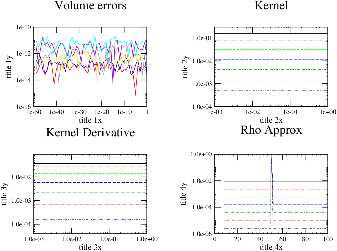
Before presenting the simulations obtained using the Cartoon SPH we verify that the construction of the virtual particles was made in a consistent way. We present four convergence tests and we present the results in Figure 2
- 1.
Volume approximation:
We check that the volume of the virtual particles and the positions assigned to them are correct. We compare for a given sphere of radius its analytical volume and the approximated value of the volume using the volumes of the virtual particles (34)
(40) where is the volume of each one of the particles. Figure 2(a) shows the behavior of the relative error () as function of the smoothing length. We can observe that the relative error is always close to the round-off error of the computer.
- 2.
Normalization of the kernel:
We verify that the relation is properly satisfied. For the i physical particle we have
(41) then, we compute the error increasing the number of virtual particles. We present the behavior in Figure 2(b).
- 3.
Derivative of the kernel:
We verify that the approximation for the derivative is satisfied. The discretization of this equation is
(42) We compute the relative error and obtain proper convergence for all the components of the derivative. We show the error of the derivative in the direction in Figure (2(c)).
- 4.
Density
The last convergence test compares the numerical approximation of a discontinuous profile of density with an initial profile () in a given region of the space:
(43) where the subindex labels the position . Again, the relative error is , and the results are presented in the figure (2(d)).
It is important to notice that if we choose a fixed number of particles and change the value of the smoothing length, the relative error remains constant.
Now we can proceed to present the main simulations used to test the cartoon implementation.
5 Blast wave
We are going to consider a spherical fluid distribution with two regions: the first one with and the second one with , here and . We are using units where .
We assume a flat spacetime properly described by the Minkowsky metric . It is clear that the lapse function is and the shift vector , . The induced on the hyper surface of constant time , ,is (the Kronecker-delta).
The parameters for the artificial viscosity are , and .
To find the initial distribution of the real particles we use equation (26)
| (44) |
with the mass contained in the inner and outer regions. In region the index takes the values and in region , .
We consider as the origin and the radius of the complete sphere. Then we can get easily the recurrence equation
- 1.
Region I:
(45) where .
- 2.
Region II:
(46) where .
5.1 The evolution
We present in the Figure (3) the physical quantities for the blast wave configuration, with the parameters mentioned above. The figure contains three different columns corresponding to three different times and . In this panels we can appreciate the behavior of the physical quantities where the velocities of the particles are very small compared with the speed of light [10].
We observe (from left to right in Figure 3) the existence of the head, rarefaction wave, tail, contact discontinuity and shock waves.
The behavior of the simulation is similar to the shock tube with some differences in the profile of the velocity between the regions of rarefaction and shock. The boundaries of the rarefaction zone are called the head and the tail, [10, 1].
The pressure is continuos in the zone between the tail and shock point (in the classical problem this is supported by the Rankine-Hugoniot conditions).
In the specific internal energy we notice a difference between the shock tube and the blast wave, in the region after the rarefaction and the contact discontinuity. All these deformations are result of the spherical symmetry of the problem.

It is clear that all the evolutions have oscillations in the area of the contact discontinuity. This is the result of the implementation of the artificial viscosity. It is important to mention that if we increase the number of real particles in the tests this oscillations decrease as we present in Figure (4) and it is because the linear interpolation is better with more subdivision in the radial direction. We used three different values of . It is also possible to used better interpolations to decrease the oscillations.

6 Conclusions
The implementation introduced in this article is a successful method that can be used to deal with problems in spherical symmetry with 3 dimensional codes instead of rewriting the equations in that symmetry. This implementation is simple and can be also applied to problems with axial symmetry. In the same way, it can also be implemented for the Newtonian Euler equations [15]. The tests we presented here, give a clear idea of the behavior of the cartoon and can be used to perform further analysis and studies of physical and astrophysical scenarios.
7 Acknowledgments
This work is supported by grants CIC-UMSNH-4.23, PROMEP UMICH-CA-22, UMICH-PTC-210 and CONACyT 79601.
References
- [1] S. Siegler and H. Riffert, Smoothed Particle Hydrodynamics Simulations of Ultrarelativistic Shocks with Artificial Viscosity, The Astrophysical Journal, 531: 1053-1066, 2000 March 10.
- [2] J.J.Monaghan, R.A.Gingold, Shock Simulation by the Particle Method, Journal of Computational Physics 52, 374-389 (1983).
- [3] J. Barnes, P. Hut, A hierarchical O(N log N) force-calculation algorithm, Nature, 324, 446-449 (1986).
- [4] V. Springel, N. Yoshida, S.D.M. White, GADGET: a code for collisionless and gas dynamical cosmological simulations, New Astronomy, 6, 2, 79-117. (2001).
- [5] S. Rosswog, Astrophysical Smooth Particle Hydrodynamics, New Astronomy Reviews, 53, 4-6, 78-104 (2009).
- [6] T. Abel, rpSPH: a much improved SPH Algorithm, Mon. Not. R. Astron. Soc. 000, 1-17 (2010).
- [7] M. Alcubierre, S. Brandt, B. Bruegmann, D. Holz, E. Seidel, R. Takahashi, J. Thornburg, Symmetry without symmetry: Numerical simulation of axisymmetric systems using Cartesian grids. Int.J.Mod.Phys.D10:273-290,2001.
- [8] J. J. Monaghan, R. A. Gingold, Shock Simulation by the Particle Method SPH, Journal of Computational Physics 52, 374-389 (1983).
- [9] J. VonNeumann, R. D. Richtmyer, A Method for the Numerical Calculation of Hydrodynamics Shocks, Journal of Applied Physics, Volume 21, March, 1950.
- [10] M. Omang, S. Borve, J. Trulsen, SPH in spherical and cylindrical coordinates, Journal of Computational Physics 213 (2006) 391-412.
- [11] S-I Inutsuka, Reformulation of SPH with Riemann Solver, Journal of Computational Physics, 179, 1, 238-267 (2002).
- [12] D. Molteni, C. Biello, Riemann Solver in SPH, Mem. S.A.It. Suppl. 1,36 (2003).
- [13] S. H. Cha, A.P. Whitworth, Implementations and tests of Godunov-type particle Hydrodynamics, Mon. Not. R. Astron. Soc. 340, 73-90 (2003).
- [14] G. R. Liu, M. B. Liu, Smoothed Particle Hydrodynamics: a meshfree particle method, World Scientific.
- [15] J. P. Cruz-Pérez, J. A. González, Using the symmetries in 3D Smoothed Particle Hydrodynamics. Submitted to AIP Conf.Proc.
- [16] C. W. Misner, K. S. Thorne, J. A. Wheeler, Gravitation, W. H. Freeman and Company.
- [17] J. R. Wilson, G. J. Mathews, Relativistic Numerical Hydrodynamics, Cambridge Monographs on Mathematical Physics.
- [18] Robert M. Wald, General Relativity, The University of Chicago Press Chicago and London.
- [19] M. Alcubierre, Introduction to 3+1 Numerical Relativity, International Series of Monographs on Physics