Rim curvature anomaly in thin conical sheets revisited
Abstract
This paper revisits one of the puzzling behaviors in a developable cone (d-cone), the shape obtained by pushing a thin sheet into a circular container of radius by a distance [1]. The mean curvature was reported to vanish at the rim where the d-cone is supported [2]. We investigate the ratio of the two principal curvatures versus sheet thickness over a wider dynamic range than was used previously, holding and fixed. Instead of tending towards 1 as suggested by previous work, the ratio scales as . Thus the mean curvature does not vanish for very thin sheets as previously claimed. Moreover, we find that the normalized rim profile of radial curvature in a d-cone is identical to that in a “c-cone” which is made by pushing a regular cone into a circular container. In both c-cones and d-cones, the ratio of the principal curvatures at the rim scales as , where is the pushing force and is the Young’s modulus. Scaling arguments and analytical solutions confirm the numerical results.
pacs
46.70.De, 68.55.-a, 46.32.+xI INTRODUCTION
When a piece of thin sheet like paper crumples, it develops a network of two types of sharp structures: straight stretching ridges and pointlike vertices. Since thin sheets and membranes are very common in both natural and man-made structures at almost all length scales, crumpling has applications in a broad range of systems, such as graphene sheets [3], carbon nanotubes [4, 5], virus capsids [6], pollen grains [7], polymerized membranes [8], and leaves [9]. The pointlike vertex singularity has mostly been studied via the simple realization known as the developable cone or d-cone, shown in Figure 1(a). A d-cone is the shape created by pushing the center of a thin sheet into a circular container of radius by a distance [1]. d-cones, stretching ridges, and crumpling in general have been studied extensively [10, 11, 12, 13, 14, 15, 16, 1, 17, 18, 19, 20, 21, 22, 23, 24, 25, 26, 27, 28, 29]. In certain cases it is possible to set bounds on the energy of singular structures [30, 31], but to our knowledge such bounds have not been established for d-cones. Furthermore, while the scaling properties of stretching ridges have been determined analytically and numerically [11, 12, 19], several phenomena in d-cones are still beyond our understanding [27]. One mysterious behavior of d-cones is the reported vanishing of mean curvature at the rim region where a d-cone is supported [2].
The deformation of a d-cone can be characterized by the deflection and its Young’s modulus is denoted by . and are defined as radial and angular components in the material coordinate system. and are the radial and azimuthal curvature respectively. In principle the shape of a d-cone is governed by the Föppl-von Kármán equations[13, 32], whose analytical solution is known only in a few special cases [33, 34]. Unfortunately, a d-cone is not one of these cases. However, it is energetically much cheaper for thin sheets to bend than to stretch, so a d-cone is asymptotically unstretched, and thence developable, except in the core region where it is pushed. Assuming that a d-cone is unstretched almost everywhere, Cerda and Mahadevan [15, 25] described the deformation in terms of the classical Elastica of Euler [35] and obtained the shape of the d-cone by minimizing the bending energy. Numerical study [24] has confirmed their finding.
 |
 |
Under the assumption that a d-cone is unstretched almost everywhere, the shape of the d-cone has zero radial curvature except in the core region, but the real shape must have nonzero at the rim to balance the normal force from the edge of the container[2, 36]. Liang and Witten [2] reported a striking feature that within numerical accuracy, as the thickness of the sheet went to zero, the radial curvature and the azimuthal curvature were nearly equal and opposite at the rim, so that the mean curvature, defined as , nearly vanished there. They found that the feature was independent of container radius , thicknesses of the sheet , and deflection , but the circular symmetry of the container was indispensable. Since nonzero entails stretching, it should be necessary to consider the stretching in the rim region in order to understand this vanishing of mean curvature feature [2].
In the limit of thin sheets, the cost of stretching becomes prohibitive and the rim region with nonzero stretching should shrink to zero. In this limit, it seems plausible to treat the rim region as a boundary layer sandwiched by regions where the Elastica approach can still be applied. This type of boundary layer phenomenon appears in a wide variety of systems, such as the Pogorelov ring ridge [32, 37], the ”minimal ridge” [12], and more recent work [38, 39, 6].
Judging from its characteristics, this vanishing mean curvature phenomenon is nonlocal and purely geometric; thus, researchers have investigated the connection between this phenomenon and another nonlocal geometric constraint on surfaces, i.e. the Gauss-Bonnet theorem[36, 40]. This theorem requires that the sum of the integral of Gaussian curvature within a surface and the integral of geodesic curvature along its boundary remain a constant. For a d-cone, the integral of geodesic curvature along the boundary can be assumed a constant, so net Gaussian curvature in one region needs to be balanced by another region(s) of opposite Gaussian curvature. Since zero mean curvature at the rim means negative Gaussian curvature, researchers have suspected the negative Gaussian curvature at the rim is necessary to balance a net positive Gaussian curvatures in the core region[36]. However, the integral of (negative) Gaussian curvature near the rim is almost completely compensated by that of two adjacent bands. Thus, the Gauss-Bonnet theorem offers no obvious explanation of the nonlocality implicit in the vanishing mean curvature phenomenon.
This paper investigates the ratio of the two principal curvatures at the rim versus sheet thickness over a wider dynamic range than was used previously in Ref. [2], holding the deflection and the container radius fixed. The numerical models are specified in Sec. II. In Sec. III, we describe our numerical findings in detail. Instead of tending towards 1 as required by the vanishing of mean curvature, the ratio at the rim goes below 1 and scales as . To better understand this power law, we study d-cone’s close cousin “c-cone” which is made by pushing a regular cone into a circular container, as seen in Figure 2(a) . C-cones are simpler structures than d-cones. In a c-cone, deflection , pushing force , and thickness are independent degrees of freedom. In both c-cones and d-cones, we find that for fixed deflection . Moreover, given the same , , and , the normalized rim profiles of radial curvature are identical in a c-cone and a d-cone. To put these numerical findings on firmer grounds, in Sec. IV we give scaling arguments for both c-cones and d-cones. General solutions for symmetrically loaded conical shells are available [41, 42], and we use the proper boundary conditions to get the analytical solutions for c-cones. Both the scaling arguments and the analytical solutions confirm the numerical results. In Sec. V, we discuss the implications of our findings.
 |
 |
II NUMERICAL METHODS
In principle, one could use standard finite element softwares such as Abaqus [43] to simulate thin sheets, but we find them difficult to adapt to the ultra-thin asymptotic behavior of d-cones that we want to study. We use an extended Seung-Nelson model [44, 19] to cope with the singularity at the center of a d-cone and to better study the interaction between the sheet and the supporting container. The extended model simulates an elastic sheet by a triangular lattice with variable lattice spacing, so it has more adaptability than the original Seung-Nelson model [45] which dictates a uniform lattice. This allows the extended model to concentrate lattice points as needed in regions of strong gradients. Our deformed lattice is shown in Figure 1(b).
The total elastic energy of the sheet is the sum of stretching and bending energies on each triangle. On an arbitrary triangle the strain tensor and curvature tensor are assumed constant. The strain tensor is determined from the changes in the edge lengths, as seen in Figure 3, and the curvature tensor from the dihedral angles between the given triangle and its three adjoining triangles as shown in Figure 4. The specific transformation formulas are derived in Appendix A. Once we know the strain and curvature tensors, we obtain the corresponding energy densities and via the conventional equations of elasticity [32, 34]:
| (1) | ||||
| (2) |
where is the Poisson’s ratio, is the bending rigidity, and is the Gaussian bending rigidity. The total elastic energy of the sheet is taken as the sum of the energy density for each triangle times its undeformed area.
 |
 |

A variable lattice for a d-cone is created in two stages [44, 19]. First a uniform triangular lattice of spacing is used to span the desired area. The lattice spacing is the distance between adjacent lattice points. Then this lattice is mapped to the desired nonuniform lattice e.g. Figure 1(b). Let the point density of the initial uniform lattice be . For our purposes we may choose a mapping with radial symmetry. For a point in the uniform lattice, we transform so its new position in the variable lattice is . Then the local point density in the variable lattice is . In practice, we choose to be a function form of , where
and the index labels the regions where local point density needs adjustment. In Figure 1(b) there are four such regions: the center region, the rim region, the region between the center and the rim, and the outer region. In the center region and the rim region the point densities are increased while in the two other larger regions the point densities are reduced. The overall average point density remains close to that of the uniform lattice before the density adjustment. As shown in Figure 5, the graph of is a simple U-shaped curve centered around , and we can control its width through and depth through .
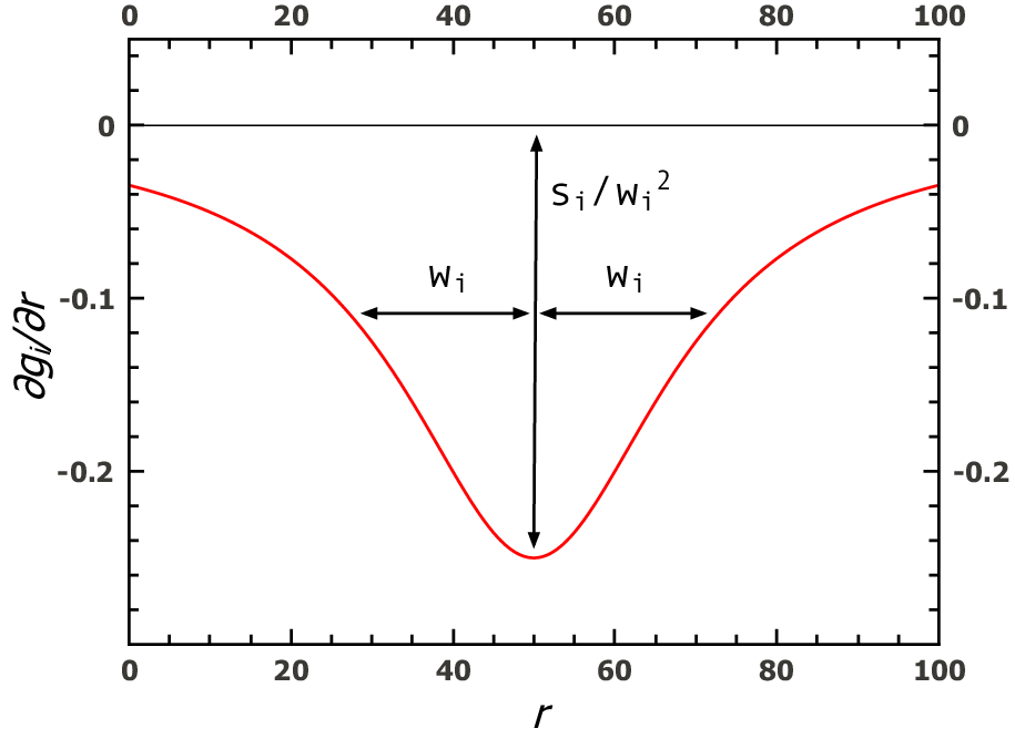
The resulting nonuniform lattice defines the initial undeformed state of Figure 3 for each triangle in the nonuniform lattice. Thus the lattice positions defined by this map constitute the state of zero stretching energy. By construction, these positions lie in a plane, so that each triangle also has zero curvature energy as defined by Figure 4.
Creating the nonuniform lattice for a c-cone requires two additional steps. To simulate a c-cone with opening angle equal to , we make a cut along the radial line , and map every lattice point through the transformation and . The last step is to join the two free boundary lines. That is, we identify each point on the free radial boundary line with its counterpart on the other free boundary line, so that the two lattice positions are constrained to occupy the same spatial position in the simulation.
The constraining container rim and the pushing force are simulated in almost the same way as previously used in Ref. [24, 36]. The rim is in the plane and its shape is determined by the equation , where is the radius of the container. We introduce an external potential to implement the geometric rim constraint for all points in the sheet. To implement such a constraint for a discrete lattice we must assure that every lattice point remains a distance of order from the rim line. For numerical tractability we assure this by adding an external potential felt by all lattice points that maintain the required separation while having negligible effect on more distant points. We find empirically that a short range potential is adequate. More specifically, we implement the repulsive normal force from the rim by introducing a potential of the form
where is a constant, is the coordinate of the th lattice point, and the summation is over the whole lattice. The value of is chosen so that the shortest distance between the lattice points and the rim is approximately the local lattice spacing in the radial direction. The potential due to the central pushing force is
Here is the coordinate of the lattice point in the center, is effectively the magnitude of the pushing force, and the function is given by
where is a constant of order . This is introduced to make sure that when the sheet is being pushed the lattice point in the center does not stray away from the axis of the cylindrical container, i.e., .
The total energy of the system is the sum of the total elastic energy in the sheet and the potential energies due to the rim and the applied pushing force. The conjugate gradient algorithm[46] is used to minimize the total energy as a function of the coordinates of all lattice points to get the final shape of the sheet [47, 24, 36]. To verify that the energy of the final configuration is at a global minimum, we can move each lattice point away from its equilibrium position by a random amount in a random direction and see if the energy minimization process will bring the system back to its original state; the magnitudes of the random displacements introduced are usually much less than the local lattice spacing. We can also check how sensitive the final configuration is to the starting configuration. A high sensitivity generally signals the thickness of the sheet is too small for the current lattice to simulate and the results are likely unreliable.
This model faithfully represents continuum sheets provided that the radii of curvature are everywhere much larger than the local lattice spacing. This limitation restricts the values of deflection to be less than or equal to in our simulations. Ref. [44] reports further details about this simulation technique. The simulation program using the nonuniform lattice has been validated to show uniform elastic behavior for states of planar stress and for cylinders. It has been validated against uniform lattices for d-cones of thickness that can be simulated by both methods. Ref. [44] also provides further simulated sheets, as well as our relaxation protocol and timing information.
Our computer program is sequential and the bottleneck of the simulation is the CPU speed. A typical d-cone or c-cone is simulated with lattice points, and it usually takes more than one month to finish the energy minimization process on a Intel Core processor. Each processor usually runs only one instance of the program at a time, but we have up to processors to run multiple instances with different parameters simultaneously.
Once the final configuration of a d-cone is obtained, the curvature tensor in each triangle can be determined using the procedure stated earlier. We then solve the characteristic equation of each curvature tensor to get the principal curvatures and . To find the radial profile of , we pick a circular sector with angle and for each triangle within this sector, its is associated with the radial coordinate of its center. As shown later, reaches its maximum at the rim where the interaction between the sheet and the container is the strongest. Within each sector we average the four largest values of near the peak as the rim value of . The four corresponding are averaged to get the rim value of . The rim curvatures depend on the angular separation between the center line of the circular sector and that of the buckled region. The angular separation is for the rim profiles of and rim values of reported in subsequent sections. The estimated percentage uncertainty of the reported rim values of due to this angular dependence is about for the whole range of thickness considered. A better approach is to average the rim and across multiple sectors, but this will have no noticeable impact on our results. Our tests also show that different initial configurations will cause at the rim to change by less than for the range of thickness considered here. If we assume these two sources of uncertainties are independent, the total percentage uncertainty for the reported rim values of should be about . The results for c-cones are determined in the same way and have the same level of uncertainties as in the d-cone data.
III NUMERICAL RESULTS
Figure 6 shows at the rim of d-cones versus relative thickness for two different values of . Unless explicitly stated otherwise, and Young’s modulus are assumed to be constant. For both and , goes below 1 as is sufficiently thin, and it does not show any sign of leveling off as it reaches as low as 0.76 in the thinnest sheets simulated. More strikingly, for each fixed , scales as . This clearly contradicts the previous observation of vanishing mean curvature which requires to stay at 1 when the sheet gets very thin. To resolve this contradiction, we need a better understanding of how at the rim responds to changes in and . However, in d-cones there is a one-to-one correspondence between and for a fixed . To gain more flexibility and to explore the generality of this feature, we study d-cone’s close relative, the c-cone.

In c-cones, for a fixed , while and are changed independently we find that at the rim scales as , as shown in Figure 7. This scaling law is justified in Section IV. In d-cones, even though and are interdependent, the same scaling law also holds. Moreover, Figure 8 demonstrates that for the same set of , , and the radial profile of normalized near the rim is the same in the d-cone as in the c-cone. These two findings together suggest very strongly that the behavior of in the rim region of a d-cone is identical to that in a c-cone, and should be explained by the same mechanism.


To shed some light on the underlying mechanism, we investigate the detailed deformation of the sheets near the supporting rim, as sketched in Figure 2(b). Let us denote the maximum deviation from the straight radial line as and the width of the deformation as . Figure 9 shows that has a linear response to and scales as . From Figure 10, we can see that is independent of and scales as . It’s worth noting that for the same and within numerical accuracy is exactly the same in a d-cone as in a c-cone. It scales in the same way as the width of a Pogorelov ring ridge formed by pushing a convex thin shell with a large inward concentrated normal force [32, 37]. Our scaling arguments in the next section will closely follow how the scaling properties of the Pogorelov ring ridge are derived.


IV SCALING ARGUMENTS AND ANALYTICAL SOLUTIONS
IV.0.1 Scaling arguments
Scaling arguments can be constructed to determine the dependence of ratio , the maximum deviation , and width on , , and . Near the rim of a c-cone or a d-cone, the energy contribution of the local deformation includes both bending and stretching energy. Let us first find how each of them scales with and .
To evaluate the bending energy component, we start with the principal curvatures. We denote quantities unperturbed by the rim force by an overbar, e.g., . We denote changes induced by the the rim force by a , e.g., . Let be the deviation of the tangent vector away from the original direction along a meridian as shown in Figure 2(b). In the deformed region and . We also have , and radius of the azimuthal curvature . Due to the local deformation, , so , or . Since as argued below, is much less than and can be safely ignored. Locally there is a contribution to the part of the bending energy of Equation 2. The change in this energy induced by the rim force is of order . However, this energy must integrate to zero because of the Gauss-Bonnet theorem. Thus the bending energy due to the local deformation near the rim (over an area ) is:
| (3) |
For the stretching component, and is negligible here 11 1 Due to the local deformation, the length of the meridian within a distance of increases by , but the stretching due to this elongation is spread over a distance much larger than . This can be shown through the following exercise. For the cone shown in Figure 2(a), let us remove the top part that is above the rim, fix the outer edge, and pull the top edge of the remaining cone along the meridian away from the outer edge by a distance of . Then and , where is the decay length of . The resulting total stretching energy will be . Minimizing this energy gives .. Thus the stretching energy contribution near the rim is:
| (4) |
Minimizing gives . Plugging this back into Equations 3 and 4, the total elastic energy is
| (5) |
Taking the derivative of the total elastic energy with respect to and equating the result to the pushing force , we find . Thus , and . All the scaling relations obtained here agree with the numerical results presented in the previous section.
IV.0.2 Analytical solutions for c-cones
The deformation of shells of revolution under symmetrical loading is a classical problem [41, 42, 48, 49]. The governing Föppl-von Kármán equations[32] are 4th order nonlinear differential equations. The analysis is greatly simplified by treating the limiting regime of weak loading, so that the equations can be linearized in the deformation. From the linearized solution, we may then verify that for loading forces of interest, the linearized treatment is completely valid for asymptotically thin sheets.
For a c-cone, assuming that the supporting container’s rim is infinitely hard (i.e. the range of the normal force from the rim is close to zero), satisfies the following differential equations as shown in Appendix B:
| (6) |
where is half of the underlying cone’s opening angle, , and .
These equations have closed form solutions in terms of Bessel functions. For , the equation is homogeneous and its general solution is [41, 42]
| (7) |
where , and a prime is differentiation with respect to . The , , , and functions are known as the Thomson or Kelvin functions [50, 42]. Evidently goes to zero for large . However, and diverges there, and are linearly independent. Thus their coefficients and must vanish. The solution for the has an extra term:
| (8) |
Even though and are divergent at , the and terms are needed to balance the term that also diverges at the apex. However, and decreases almost exponentially as increases, so these two terms are negligible near the rim. For our purpose of getting the radial profile of near the rim, the term can also be ignored because it changes in length scale , which is much larger than the width of the rim region. The contribution of this term to at the rim is vanishingly small compared with the we got from numerical simulations and scaling arguments:
| (9) |
We conclude from the preceding reasoning that it is sufficient to specify , , , and for the inner and outer regions. To determine these four coefficients, we may use the four matching conditions applicable at the forcing point : is continuous and equal to zero , the curvature is also continuous, and there is a jump for which equals . The last condition is due to the assumption that the rim of the supporting container is infinitely hard. Any localized force on an elastic sheet produces a discontinuity of curvature derivative of this type [32].
Finally, we can compare the radial profile of from analytical solution with that from numerical simulation. The overall excellent agreement between them, as shown in Figure 11, gives convincing evidence that our numerical results are valid. It should be stressed that there is no normalization in either axis. The difference between the peak values are primarily due to three factors. First, as noted in Section II the percentage uncertainty of the rim curvatures from simulation is about . Second, the analytical solution assumes an infinitely sharp container edge, but the force range of the normal force used in the simulation is close to of the full-width-at-half-maximum (FWHM) of the peak for this specific c-cone. Third, the local lattice spacing in the radial direction is also about of the FWHM. The last two factors cause the simulated curve to have a rounded peak. The effect of the finite thickness of the sheet is negligible here since the thickness is less than a tenth of the normal force range. Finite size of the simulation can also influence the curvature profile.
In addition to the stronger peak, the analytical solution shown in Figure 11 has a stronger dip on either side. We believe this is due to the local compensation of Gaussian curvature [36], which requires the integral under the curve to be zero. So if the analytical solution has extra area under the peak, it must have extra negative area at the dips.
Over the full range of the c-cone sheet thickness covered in our simulation, the peak values of the at the rim from simulation is lower than that given by the analytical solutions by between and . We should expect a similar level of discrepancy between the simulation and analytical solutions for the d-cone. Thus the lowest value achieved for d-cones in our simulations may increase from to a value as high as , which is much closer to , but this level of discrepancy should have no material impact on the scaling relationship between , , and , which is the much stronger evidence that at the rim will drop below one and keep decreasing as the thickness of the sheet approaches zero.

V DISCUSSION AND CONCLUSION
In this paper we have shown numerically that contrary to previous claims, the mean curvature at the rim in a d-cone does not vanish as the thickness of the sheet goes to zero. This vanishing requires that goes to . However, in the range we studied, at the rim appears to vary as . More generally, in both c-cones and d-cones, . These identical scaling laws and the similarity of the radial profiles of in d-cones and c-cones suggest that the core region of a d-cone has no influence on how the rim region reacts to the normal rim force pressure. The core region only affects the amplitude of the rim force pressure.
This paper does not attempt to determine the right scaling law for the pushing force in a d-cone. Simply combining the derived scaling law with the numerically observed scaling law for will give . There is another proposed functional form for : , where is radius of the sheet, and is the radius of the core region [25, 1]. The first force scaling is asymptotically much stronger than the second one with the logarithmic term. However, within the dynamic range covered in our simulations, the fit for these two functional forms are equally good. It should also be mentioned that some researchers have expressed doubts on the arguments leading to the second functional form[24, 27]. Our work in progress aims to resolve this issue.
Acknowledgments
The author is grateful to Thomas A. Witten for enlightening discussions. He warmly thanks the University of Chicago Computer Science Instructional Laboratories for providing computing resources. This work was performed as part of the author’s PhD research under the supervision of Thomas A. Witten and was supported in part by the US-Israel Binational Science Foundation and in part by the National Science Foundation’s MRSEC Program under Grant Number DMR 0820054.
Appendix A Formulas for strain and curvature tensors
A.1 Formulas for the strain tensor
This subsection derives the expression for strain tensor in terms of the changes of edge lengths , and in an arbitrary triangle as shown in Figure 3(a) and 3(b).
In Figure 3(a), let the coordinates of , , and be , , and , respectively. When triangle is under strain, as shown in Figure 3(b), denote the changes of , , and as , , and , and the new coordinates of , , and are , , and . For a general point in the triangle, let us denote its displacement as , so its coordinate due to deformation is . Under the assumption of infinitesimal constant strain across the triangle, , , , and should be constants. We can also expand the displacement of points and in terms of these partial derivatives:
| (10) | ||||
| (11) | ||||
| (12) | ||||
| (13) |
Ignoring the higher order terms, we can solve Equations 10, 11,12,and 13 for , , , and :
| (14) | ||||
| (15) | ||||
| (16) | ||||
| (17) |
Then we can easily get the strain tensor elements [32]:
| (18) | ||||
| (19) | ||||
| (20) |
or in matrix form:
| (21) |
where
| (22) |
We have determined the elements of in terms of , , and , but it is much more efficient to compute , , and during simulating, so let us find the expression for , , and in terms of , , and , and then express in terms of , , and .
A.2 Formulas for the curvature tensor
To calculate the curvature tensor on an arbitrary triangle, e.g. triangle in Figure 4, we can fit the coordinates of the six vertices of its three adjoining triangles to the following function [19, 24]:
| (29) |
where are coordinates of the vertices in a local coordinate system. In this system, the axis is perpendicular to and its origin is at the center of . These choices ensure that and are negligible. Then the curvature tensor elements are determined through [19, 24]
| (30) |
If we ignore the changes in the and , the coefficient matrix in Equation 29 will stay the same during the simulation, which means for each triangle we only need to invert the coefficient matrix once at program initialization. Under the assumption that both bending and stretching are infinitesimal, this simplification will result in a second order error in the curvature tensor.
In this local coordinate system, , , and are all zero by the choice of the axis. The other three nonzero coordinates , , and can be determined from the three dihedral angles between and its three adjoining neighbors. For example, , where is the distance from point to edge . So, alternatively, we can also determine the curvature tensor from the three dihedral angles , , and .
This method works for both uniform and variable lattices.
Appendix B Analytical solutions for c-cones

Ref. [42] provides detailed information on the general theory of symmetrically loaded shells of revolution, including conical shells. Its derivation assumes that the deformation is small relative to the size of the structure, but may be comparable to the thickness. In this regime, both bending and in-plane stretching may occur and thus need to be considered together. However, for many problems only the force and moment balance of the undistorted element is needed, and the resulting equations are normally linear. Here, we will simply quote the relevant equations presented in Ref. [42] and use them to find the specific equations for c-cones assuming that the supporting container’s rim is infinitely hard.
As shown in Figure 12, , , and are the pressure, axial and radial forces per unit length, respectively. is the radial distance from the axis and it is related to through . In a conical shell these variable and satisfy the following equations according to Ref. [42]:
| (31) |
| (32) |
| (33) |
where is a constant of integration. It is worth noting that these equations are derived for sheets whose unstressed (or undeformed) state has curvature, but we find that they are also valid when the unstressed state is flat.
Since we assume the supporting container’s rim is infinitely hard, using the balance of force it is straightforward to determine that in c-cones has the following functional form:
| (34) |
where is the Heaviside step function. Combining Equations 31 and 34, we can get:
| (35) |
where is the Dirac delta function. Plugging this into Equations 32 and 33 and replacing with yield:
| (36) |
| (37) |
Equation 36 can be rewritten to get an explicit expression for :
| (38) |
References
- [1] E. Cerda, S. Chaïeb, F. Melo, and L. Mahadevan, Nature 401, 46 (1999).
- [2] T. Liang and T. A. Witten, Phys. Rev. E 73, 046604 (2006).
- [3] A. Fasolino, J. H. Los, and M. I. Katsnelson, Nature Materials 6, 858 (2007).
- [4] A. Cao, P. L. Dickrell, W. G. Sawyer, M. N. Ghasemi-Nejhad, and P. M. Ajayan, Science 310, 1307 (2005).
- [5] I. Arias and M. Arroyo, Phys. Rev. Lett. 100, 085503 (2008).
- [6] J. Lidmar, L. Mirny, and D. R. Nelson, Phys. Rev. E 68, 051910 (2003).
- [7] E. Katifori, S. Alben, E. Cerda, D. R. Nelson, and J. Dumais, PNAS 107, 7635 (2010).
- [8] L. Pocivavsek, R. Dellsy, A. Kern, S. Johnson, B. Lin, K. Y. C. Lee, and E. Cerda, Science 320, 912 (2008).
- [9] H. Liang and L. Mahadevan, PNAS 106, 22049 (2009).
- [10] T. A. Witten and H. Li, Europhys. Lett. 23, 51 (1993).
- [11] A. Lobkovsky, S. Gentges, H. Li, D. Morse, and T. A. Witten, Science 270, 1482 (1995).
- [12] A. E. Lobkovsky and T. A. Witten, Phys. Rev. E 55, 1577 (1997).
- [13] M. Ben Amar and Y. Pomeau, Roy. Soc. Lond. A 453, 729 (1997).
- [14] S. Chaïeb, F. Melo, and J.-C. Géminard, Phys. Rev. Lett. 80, 2354 (1998).
- [15] E. Cerda and L. Mahadevan, Phys. Rev. Lett. 80, 2358 (1998).
- [16] S. Chaïeb and F. Melo, Phys. Rev. E 60, 6091 (1999).
- [17] A. Boudaoud, P. Patricio, Y. Couder, and M. Ben Amar, Nature 407, 718 (2000).
- [18] T. Mora and A. Boudaoud, Europhys. Lett. 59, 41 (2002).
- [19] B. A. DiDonna, Phys. Rev. E 66, 016601 (2002).
- [20] E. Hamm, B. Roman, and F. Melo, Phys. Rev. E 70, 026607 (2004).
- [21] E. Cerda, L. Mahadevan, and J. M. Pasini, PNAS 101, 1806 (2004).
- [22] S. Farmer and C. Calladine, International Journal of Mechanical Sciences 47, 509 (2005).
- [23] D. L. Blair and A. Kudrolli, Phys. Rev. Lett. 94, 166107 (2005).
- [24] T. Liang and T. A. Witten, Phys. Rev. E 71, 016612 (2005).
- [25] E. Cerda and L. Mahadevan, Proc. R. Soc. A 461, 671 (2005).
- [26] C. A. Andresen, A. Hansen, and J. Schmittbuhl, Phys. Rev. E 76, 026108 (2007).
- [27] T. A. Witten, Rev. Mod. Phys. 79, 643 (2007).
- [28] H. Aharoni and E. Sharon, Nature Materials 9, 993 (2010).
- [29] P. Mellado, S. Cheng, and A. Concha, Phys. Rev. E 83, 036607 (2011).
- [30] S. C. Venkataramani, Nonlinearity 17, 301 (2004).
- [31] S. Conti and F. Maggi, Archive for Rational Mechanics and Analysis 187, 1 (2008).
- [32] L. D. Landau and E. M. Lifshitz, Theory of Elasticity (Pergamon Press, New York, 1986).
- [33] A. E. Lobkovsky, Phys. Rev. E 53, 3750 (1996).
- [34] E. H. Mansfield, The Bending and Stretching of Plates (Pergamon, New York, 1964).
- [35] C. G. Fraser, Centaurus 34, 211 (1991).
- [36] J. W. Wang and T. A. Witten, Phys. Rev. E 80, 046610 (2009).
- [37] A. Pogorelov, Bendings of surfaces and stability of shells, Translations of mathematical monographs (American Mathematical Societ, Providence, R.I, 1988).
- [38] B. Audoly, Phys. Rev. Lett. 83, 4124 (1999).
- [39] W. Jin and R. Kohn, Journal of Nonlinear Science 10, 355 (2000).
- [40] D. J. Struik, Lectures on Classical Differential Geometry (Addison-Wesley Publishing Company, Massachusetts, 1961).
- [41] A. Love, A Treatise on the Mathematical Theory of Elasticity (Dover Publications, New York, 1944), 4th ed.
- [42] C. E. Turner, Introduction to Plate and Shell Theory (American Elsevier Publishing Company, 1965).
- [43] Abaqus Theory Manual (6.9), Dassault Systèmes Simulia Corp., Providence, RI (2009).
- [44] J. W. Wang and T. A. Witten, manuscript in preparation.
- [45] H. S. Seung and D. R. Nelson, Phys. Rev. A 38, 1005 (1988).
- [46] W. H. Press, S. A. Teukolsky, W. T. Vetterling, and B. P. Flannery, Numerical Recipe in C (Cambridage University Press, Cambridage, 1996).
- [47] I. M. Jánosi, D. Chrétien, and H. Flyvbjerg, European Biophysics Journal 27, 501 (1998).
- [48] J. E. Gibson, Linear Elastic Theory of Thin Shells (Pergamon Press, 1965).
- [49] W. Flügge, Stresses in Shells (Springer-Verlag, Berlin, 1960).
- [50] G. N. Watson, A Treatise on the Theory of Bessel Functions (Cambridge University Press, 1944), 2nd ed.