1Introduction

IGC–11/5–1

Black-hole horizons in modified space-time structures arising from canonical quantum gravity

Martin Bojowald,¹^*^* * e-mail address: bojowald@gravity.psu.edu George M. Paily,¹^†^† † e-mail address: gmpaily@phys.psu.edu Juan D. Reyes^2,3^‡^‡ ‡ e-mail address: jdreyes@matmor.unam.mx and Rakesh Tibrewala⁴^§^§ § e-mail address: rtibs@imsc.res.in

¹Institute for Gravitation and the Cosmos, The Pennsylvania State University,

104 Davey Lab, University Park, PA 16802, USA

²Instituto de Matemáticas,

Universidad Nacional Autónoma de México, Campus Morelia,

A. Postal 61-3, C.P. 58090, Morelia, Michoacán, Mexico

³Instituto de Física y Matemáticas,

Universidad Michoacana de San Nicolás de Hidalgo,

Edificio C-3, Ciudad Universitaria, Morelia, Michoacán, Mexico

⁴The Institute of Mathematical Sciences, CIT Campus, Chennai 600113, India

Abstract

Several properties of canonical quantum gravity modify space-time structures, sometimes to the degree that no effective line elements exist to describe the geometry. An analysis of solutions, for instance in the context of black holes, then requires new insights. In this article, standard definitions of horizons in spherical symmetry are first reformulated canonically, and then evaluated for solutions of equations and constraints modified by inverse-triad corrections of loop quantum gravity. When possible, a space-time analysis is performed which reveals a mass threshold for black holes and small changes to Hawking radiation. For more general conclusions, canonical perturbation theory is developed to second order to include back-reaction from matter. The results shed light on the questions of whether renormalization of Newton’s constant or other modifications of horizon conditions should be taken into account in computations of black-hole entropy in loop quantum gravity.

1 Introduction

Canonical quantum gravity allows for new quantum space-time structures to replace the classical continuum underlying general relativity. If new forms of space-time are realized, they must come along with a modified version of general covariance embodied in the set of transformations acting on them. Covariance in this general sense is encoded in the constraint algebra of a gravitational theory under consideration, which can easily acquire quantum corrections. Provided the quantum constraints form a first-class algebra, covariance is not broken but might be modified compared to the classical notion. Many of the standard effects of space-time are then expected to change; this article provides an exploration in the context of black-hole aspects. (Qualitatively, there are similarities to deformed Poincaré symmetries [1], but a detailed relationship is not straightforward to work out.)

Loop quantum gravity [2, 3, 4] has provided a discrete notion of quantum space, subject to dynamical laws. Several key properties of this kind of quantum geometry have implications that can be implemented consistently at the level of modified classical constraints, especially in the spherically symmetric context. The general theory is not unique, and so several different types of modifications are possible. But many characteristic features arise in a way rather insensitive to quantization ambiguities, which are then interesting to probe in concrete models. In this article, we focus on corrections arising from the quantization of inverse components of the triad variables used in loop quantum gravity. They imply corrections in the Hamiltonian constraint [5] which change the dynamics and, generically, the constraint algebra of effective geometries. In this special case of spherical symmetry, also versions of corrected constraints not changing the algebra exist, which provide interesting comparisons.

We use these examples to probe possible influences of quantum space-time on properties of non-rotating black holes. Concrete scenarios of collapse or evaporation sensitive to global space-time structure cannot be considered reliable at the present stage of developments, but an exploration of general aspects is worthwhile. Among them are: the form of solutions, the status of different gauges, and direct implications for black holes such as horizons, Hawking radiation, or singularities. Many of the classically known properties can no longer be taken for granted when even the notion of space-time has changed. The examples provided here thus show some of the expectations toward quantum gravity in general, as well as the way in which loop quantum gravity at present can deal with them.

In particular, we will see that classical horizon conditions require modifications in order to produce dynamically consistent results in the presence of quantum-gravity corrections. Section 2 introduces the corrections and discusses their consistency. In Section 3 we find and analyze background solutions analogous to the Schwarzschild and Painlevé–Gullstrand forms of space-time. Section 4 is devoted to second-order perturbation theory in canonical form, directly applicable to corrected constraints encoding modified space-time structure. Section 5, finally, applies this perturbation theory to horizon conditions with the main result: Classical horizon conditions can consistently be used when constraints are corrected but obey the classical algebra. When the constraint algebra is modified, however, classical horizon conditions become inconsistent and gauge-dependent. We will provide modifications of the horizon conditions so as to make them consistent in the cases considered here. The area-mass relation of horizons is corrected in both cases of corrected constraints, with modified and unmodified constraint algebra. In the final section we will discuss implications for black-hole entropy calculations in loop quantum gravity, which so far use the classical conditions after an implicit gauge fixing implied by implementing the horizon as a boundary.

2 Models in Connection Variables

We recall that the canonical set of variables used for a loop quantization of gravity consists of the $\mathfrak{su}(2)$ -valued Ashtekar–Barbero connection $A_{a}^{i}(\bar{x})$ and a densitized triad $E^{a}_{i}(\bar{x})$ (which can be seen as an $\mathfrak{su}(2)$ -valued densitized vector field) on a 3-dimensional manifold coordinatized by $\bar{x}$ . (Here Latin indices $a,b,\ldots$ from the beginning of the alphabet are space indices and those from the middle of the alphabet $i,j,\ldots$ are internal indices.)

Classically, one gives a geometrical interpretation to these quantities through their relation with the standard geometrical variables used in the Hamiltonian formulation of general relativity: the Riemannian metric $q_{ab}$ on space-like hypersurfaces embedded in spacetime with normal $n^{a}$ , and the corresponding extrinsic curvature

K_{ab}=\frac{1}{2}\mathcal{L}_{n}q_{ab}\,.

(1)

The spatial 3-dimensional metric $q_{ab}$ is constructed from the densitized triad via $(\det q)q^{ab}=E_{i}^{a}E_{i}^{b}$ , while the Ashtekar–Barbero connection [6, 7] is related to the extrinsic curvature and the spin connection $\Gamma^{i}_{a}$ compatible with the triad by the formula

A^{i}_{a}=\Gamma^{i}_{a}+\gamma K^{i}_{a}\,,

(2)

where $K^{i}_{a}:=|\det E|^{-\frac{1}{2}}K_{ab}E^{bi}$ and $\gamma>0$ is the Barbero-Immirzi parameter [7, 8]. Its value, estimated by calculations of black-hole entropy [9, 10], is usually reported as $\gamma\sim 0.24$ [11]. To that end, one treats the horizon as a boundary of space-time and imposes isolated-horizon conditions for the boundary fields. The boundary fields are then quantized and configurations giving rise to a certain value of the area are counted. Details of this procedure are still being developed [12, 13, 14, 15, 16, 17, 18] but the basic premise of using classical horizon conditions to set up the quantum theory has not been questioned. Later in this article we will come back to the consistency issue arising from the fact that a classical condition for horizons is imposed before quantization.

We will simplify the dynamical discussion by working with a midisuperspace model. Imposing spherical symmetry [19, 20] and using adapted coordinates $(t,x,\vartheta,\varphi)$ reduces the SU(2)-gauge of the original variables to U(1). The densitized triad is then determined by two U(1)-invariant functions $E^{x}(x)$ and $E^{\varphi}(x)$ and a pure gauge angle $\eta(x)$ . This gauge angle also determines the $x$ -component of the spin connection $\Gamma_{x}=-\eta^{\prime}$ , while its ‘angular’ gauge-invariant component is $\Gamma_{\varphi}=-E^{x}\,{}^{\prime}/2E^{\varphi}$ (for details see [21, 22]). Here and in what follows the prime denotes a derivative with respect to the radial coordinate $x$ , while a dot will denote derivatives with respect to the time coordinate $t$ . The spherically symmetric metric in terms of these variables is

{\rm d}s^{2}=-N^{2}{\rm d}t^{2}+\frac{E^{\varphi}\,{}^{2}}{|E^{x}|}({\rm d}x+N^{x}{\rm d}t)^{2}+|E^{x}|{\rm d}\Omega^{2}

(3)

where $N(t,x)$ is the lapse function and $N^{x}(t,x)$ the only nonzero component of the shift vector.

Similarly the Ashtekar connection is determined by three functions: a U(1)-connection $A_{x}(x)$ , a U(1)-invariant function $A_{\varphi}(x)$ and the gauge angle $\eta(x)-\alpha(x)$ . The relation (2) then gives [22]

A_{\varphi}\cos\alpha=\gamma K_{\varphi}\quad,\quad A_{x}+\eta^{\prime}=\gamma K_{x}\quad\mbox{and}\quad A_{\varphi}^{2}=\Gamma_{\varphi}^{2}+\gamma^{2}K_{\varphi}^{2}

for the gauge invariant parts $K_{x}$ and $K_{\varphi}$ of extrinsic curvature. A suitable choice of variables for a loop quatization of spherically reduced gravity gives the symplectic structure:

\{A_{x}(x),\frac{1}{2\gamma}E^{x}(y)\}=\{K_{\varphi}(x),E^{\varphi}(y)\}=\{\eta(x),\frac{1}{2\gamma}P^{\eta}(y)\}=G\delta(x,y)

where $P^{\eta}:=2A_{\varphi}E^{\varphi}\sin\alpha$ is the conjugate momentum of the gauge angle $\eta$ .

Imposing the Gauss constraint

G_{\rm grav}[\lambda]=\frac{1}{2G\gamma}\int{\mathrm{d}}x\,\lambda((E^{x})^{\prime}+P^{\eta})\,,

the generator of the residual U(1)-gauge transformations of the theory, we may further eliminate $\eta$ and $P^{\eta}$ and work with the canonical pairs:

\{K_{x}(x),E^{x}(y)\}=2G\delta(x,y)\quad\mbox{and}\quad\{K_{\varphi}(x),E^{\varphi}(y)\}=G\delta(x,y)\,.

(4)

2.1 Constraints and corrections

In these variables, the constraints of general relativity (including generic matter contributions $\rho$ and $J_{x}$ for the energy density and flux) take the following forms:

Hamiltonian Constraint

\mathbf{H}[N]=-\frac{1}{2G}\int{\mathrm{d}}x\,N|E^{x}|^{-\frac{1}{2}}\bigg[K_{\varphi}^{2}E^{\varphi}+2K_{\varphi}K_{x}E^{x}+(1-\Gamma_{\varphi}^{2})E^{\varphi}+2\Gamma_{\varphi}^{\prime}E^{x}-8\pi GE^{\varphi}|E^{x}|\rho\bigg]\approx 0

(5)

Diffeomorphism constraint

\mathbf{D}[N^{x}]=\frac{1}{2G}\int{\mathrm{d}}x\,N^{x}\bigg[2E^{\varphi}K_{\varphi}^{\prime}-K_{x}E^{x^{\prime}}-8\pi GE^{\varphi}\sqrt{|E^{x}|}J_{x}\bigg]\approx 0

(6)

Under the conditions of the space-time being static, these constraints and the equations of motion they generate can be solved to give the traditional Schwarzschild metric, and similarly, the Painlevé–Gullstrand metric, which describes the same situation in different coordinates. We will demonstrate some of the derivations below, including also one type of quantum corrections. The corrections discussed here are inspired by calculations in loop quantum gravity, but we will attempt to keep our conclusions as general as possible. For the rest of this work we will use units where the gravitational constant $G=1$ .

Quantizing gravity is expected to lead to different types of quantum corrections of the constraints. They are often subject to quantization ambiguities, but requiring the new constraints to still have an anomaly-free first class algebra puts restrictions on the general form of the corrections. Anomaly-freedom, however, is not always easy to achieve, and so it is useful to split an analysis of quantum-gravity corrections into the different types. Even a single type of correction, while not providing complete equations, can put strong consistency conditions on the formalism. In loop quantum gravity, it turns out that the easiest corrections to implement are the inverse triad corrections, which arise when one quantizes terms in the Hamiltonian constraint containing inverse components of the densitized triad. In this framework, the $E^{a}_{i}$ are quantized to flux operators with discrete spectra containing zero [23, 24]. Since such operators do not have densely defined inverses, no direct inverse operator is available. Instead well-defined techniques [5, 25] are used that imply corrections (generally denoted as $\alpha$ in what follows) to the classical inverse.

A basic condition on $\alpha$ is that it be a scalar to preserve the spatial transformation properties of the corrected expressions. Among the triad variables, $E^{x}$ is the only one with density weight zero, and thus we can restrict $\alpha$ to depend only on $E^{x}$ . In the actual operators, $E^{x}(x)$ appears via fluxes, integrated over small plaquettes forming the scaffolding of a discrete quantum state, not via the whole orbit area $4\pi|E^{x}|$ at radius $x$ . Qualitatively, the correction function is a function $\alpha(\Delta)$ depending on $E^{x}$ via the plaquette size $\Delta=E^{x}/{\cal N}(E^{x})$ , obtained by dividing the orbit size by the number of plaquettes ${\cal N}(E^{x})$ that form an orbit of size $|E^{x}|$ . In general, the number must be assumed to be a function of $E^{x}$ since a large orbit has to contain more plaquettes than a smaller one in order to provide a similar microscopic scale; this refinement of the underlying discrete structure as the orbit considered grows is analogous to lattice refinement in an expanding universe [26, 27]. As in homogeneous models, lattice refinement cannot be fully derived within a pure midisuperspace setting; the freedom must thus be suitably parameterized.

A concrete calculation of correction functions results in [28]

\alpha(\Delta)=2\sqrt{\Delta}\frac{\sqrt{|\Delta+\gamma\ell_{\mathrm{P}}^{2}/2|}-\sqrt{|\Delta-\gamma\ell_{\mathrm{P}}^{2}/2|}}{\gamma\ell_{\mathrm{P}}^{2}}

(7)

with the Planck length $\ell_{\mathrm{P}}$ (see Fig. 1). (Quantization ambiguities imply that the functional form is not uniquely fixed, but the qualitative properties used here are robust.) For a small range of orbit radii and short evolution times, as suitable for quasilocal horizon properties, one may assume ${\cal N}$ to be a constant, whose sole effect then is to raise the quantum-gravity scale for $E^{x}$ where inverse-triad corrections become important from $\ell_{\mathrm{P}}^{2}$ to ${\cal N}\ell_{\mathrm{P}}^{2}$ . These corrections are thus relevant not just for Planck-size spheres; what matters is how close the size of elementary plaquettes is to the Planck scale.

Refer to caption — Figure 1: The correction function $\alpha(\Delta)$ where $\Delta$ is taken relative to $\Delta_{*}:=\sqrt{\gamma{\cal N}/2}\ell_{\mathrm{P}}$ .

In particular, including a gauge choice for $E^{x}$ we shall consider the following situation:

E^{x}=x^{2}\quad,\quad\alpha=2x\frac{\sqrt{|x^{2}+\gamma{\cal N}\ell_{\mathrm{P}}^{2}/2|}-\sqrt{|x^{2}-\gamma{\cal N}\ell_{\mathrm{P}}^{2}/2|}}{\gamma{\cal N}\ell_{\mathrm{P}}^{2}}\,.

(8)

As appropriate, we will comment throughout the paper on the reliability of our conclusions in light of the fact that not all possible quantum-gravity corrections are being considered.

The modified gravitational part of the Hamiltonian constraint we consider here is

	$\displaystyle H^{Q}_{\rm grav}[N]=-\frac{1}{2G}\int{\mathrm{d}}x\,N\bigg[$	$\displaystyle\alpha\|E^{x}\|^{-\frac{1}{2}}K_{\varphi}^{2}E^{\varphi}+2\bar{\alpha}K_{\varphi}K_{x}\|E^{x}\|^{\frac{1}{2}}+$
		$\displaystyle+\alpha\|E^{x}\|^{-\frac{1}{2}}(1-\Gamma_{\varphi}^{2})E^{\varphi}+2\bar{\alpha}\Gamma_{\varphi}^{\prime}\|E^{x}\|^{\frac{1}{2}}\bigg]$		(9)

with corrections of different powers of $E^{x}$ left independent by using, for the sake of generality, two correction functions $\alpha$ and $\bar{\alpha}$ . (Also $\Gamma_{\varphi}$ might initially be expected to be corrected with independent correction functions, but no such anomaly-free version exists [29].) There is no inverse triad component in the diffeomorphism constraint, and its action is directly represented on graph states by the spatial deformations it generates. Thus, we will keep the diffeomorphism constraint unmodified.

The Poisson algebra of modified constraints closes:

	$\displaystyle\{H_{\rm grav}^{Q}[N],D_{\rm grav}[N^{x}]\}$	$\displaystyle=$	$\displaystyle-H_{\rm grav}^{Q}[N^{x}N^{\prime}]\,,$		(10)
	$\displaystyle\{H_{\rm grav}^{Q}[N],H_{\rm grav}^{Q}[M]\}$	$\displaystyle=$	$\displaystyle D_{\rm grav}[\bar{\alpha}^{2}\|E^{x}\|(E^{\varphi})^{-2}(NM^{\prime}-MN^{\prime})]\,.$		(11)

The Poisson bracket relations (11) (or (20) below in the presence of scalar matter) with $\bar{\alpha}=1$ express the fact that dynamics takes place on space-like hypersurfaces embedded in a pseudo-Riemannian spacetime [30]. However, for generic $\bar{\alpha}\neq 1$ , this algebra no longer coincides with the algebra of spherically symmetric hypersurface deformations of general relativity and generally spacetime covariant systems.¹¹ 1 Defining $\bar{\alpha}N=\bar{N}$ , we have $\bar{\alpha}^{2}(NM^{\prime}-MN^{\prime})=(\bar{N}\bar{M}^{\prime}-\bar{M}\bar{N}^{\prime})$ and the algebra can formally be written in classical form $\{H_{\rm grav}^{Q}[\bar{N}/\bar{\alpha}],H_{\rm grav}^{Q}[\bar{M}/\bar{\alpha}]\}=D_{\rm grav}[|E^{x}|(E^{\varphi})^{-2}(\bar{N}\bar{M}^{\prime}-\bar{M}\bar{N}^{\prime})]$ . However, using $\bar{N}$ in the full algebra will then modify the Poisson bracket (10) of the Hamiltonian with the diffeomorphism constraint. The algebra is a fundamental object, encoding not only gauge properties of gravity but the structure of spacetime as well. Thus, for $\bar{\alpha}\neq 1$ not only the dynamics (reflected by the modified Hamiltonian constraint (9)) but also the structure or symmetries of the spacetime manifold are changed by these quantum corrections. Gauge symmetries will, in general, no longer coincide with coordinate transformations in our models and we cannot interpret the dynamical fields $E^{x}$ and $E^{\varphi}$ as components of a pseudo-Riemannian metric as in (3): modified gauge transformations of $E^{x}$ and $E^{\varphi}$ no longer match with coordinate transformations of ${\rm d}x^{\mu}$ to form an invariant ${\rm d}s^{2}$ . (Possible candidates for space-time models corresponding to the corrected gauge transformations are non-commutative manifolds or Finsler geometries. The latter can be explored in this context using the formalism of [31].)

We will consider in detail the two cases $\alpha\not=\bar{\alpha}=1$ and $\alpha=\bar{\alpha}\not=1$ . All other cases where

1\neq\alpha\neq\bar{\alpha}\neq 1

(12)

can formally be related to the solutions with $\bar{\alpha}=1$ by means of the substitutions

N\rightarrow\frac{N_{\alpha}}{\bar{\alpha}};\quad\alpha\rightarrow\frac{\alpha}{\bar{\alpha}}.

(13)

where $N_{\alpha}$ refers to the value of $N$ in the $\bar{\alpha}=1$ case. (We will keep matter terms general, referring only to the energy density and energy flow without specific matter models. Thus, the substitution will lead to different matter terms compared to the case with $\bar{\alpha}=1$ , but will not change the analysis of equations.) Note, however, that since $\bar{\alpha}\neq 1$ in the original constraints, the system is not generally covariant and coordinate transformations between the different gauges do not exist.

For the first choice, the Hamiltonian constraint is replaced by its modified counterpart (9) with $\bar{\alpha}=1$ , while the diffeomorphism constraint (6) remains unchanged, as does the overall form of the constraint algebra. How does this first type of modification square with the result [30, 32] that given the constraint algebra of classical general relativity, the Hamiltonian that depends only on the 3-metric and the extrinsic curvature is uniquely the classical Hamiltonian of general relativity? First note that while the relations (4) still hold, we can no longer interpret $K_{a}$ as extrinsic curvatures of the metric. This can be easily seen from the equation for $K_{x}$ derived from the corrected evolution equations, (22) and (23) below. Classically, we have:

K_{x}=\frac{1}{N}\bigg(\frac{\dot{E}^{\varphi}}{\sqrt{|E^{x}|}}-\frac{E^{\varphi}\dot{E}^{x}}{2|E^{x}|^{3/2}}+\frac{N^{x}E^{\varphi}(E^{x})^{\prime}}{2|E^{x}|^{3/2}}-\frac{(N^{x}E^{\varphi})^{\prime}}{\sqrt{|E^{x}|}}\bigg)

(14)

but with the modified equations we get:

K_{x}=\frac{1}{N}\bigg(\frac{\dot{E}^{\varphi}}{\sqrt{|E^{x}|}}-\frac{\alpha E^{\varphi}\dot{E}^{x}}{2|E^{x}|^{3/2}}+\frac{N^{x}\alpha E^{\varphi}(E^{x})^{\prime}}{2|E^{x}|^{3/2}}-\frac{(N^{x}E^{\varphi})^{\prime}}{\sqrt{|E^{x}|}}\bigg)

(15)

which cannot be derived from relation (1). The component $K_{\varphi}=(\dot{E}^{x}-N^{x}(E^{x})^{\prime})/2N\sqrt{|E^{x}|}$ is not modofied if $\bar{\alpha}=1$ . We can relate the $\alpha$ -modified $K_{a}$ , which are conjugate to the densitized triad, to the geometric extrinsic curvature components from (1), denoted here by $\bar{K}_{a}$ :

K_{\varphi}=\bar{K}_{\varphi}\quad,\quad K_{x}=\bar{K}_{x}-\frac{(\alpha-1)E^{\varphi}}{E^{x}}\bar{K}_{\varphi}.

(16)

Substituting this into (9), we get the following Hamiltonian in terms of the densitized triad and the extrinsic curvatures:

	$\displaystyle H^{Q}_{\rm grav}[N]=-\frac{1}{2G}\int{\mathrm{d}}x\,N\bigg[$	$\displaystyle(2-\alpha)\|E^{x}\|^{-\frac{1}{2}}\bar{K}_{\varphi}^{2}E^{\varphi}+2\bar{K}_{\varphi}\bar{K}_{x}\|E^{x}\|^{\frac{1}{2}}+$
		$\displaystyle+\alpha\|E^{x}\|^{-\frac{1}{2}}(1-\Gamma_{\varphi}^{2})E^{\varphi}+2\Gamma_{\varphi}^{\prime}\|E^{x}\|^{\frac{1}{2}}\bigg]$		(17)

The Hamiltonian constraint is thus modified also in the geometrical variables $\bar{K}_{a}$ which correspond to the classical form of extrinsic curvature but are no longer canonically conjugate to the densitized triads. Compared with the full situation [30, 32], the constraint algebra in spherical symmetry is thus not as restrictive, and different sets of constraints can give rise to the same algebra.

2.2 Matter fields

For concreteness, we consider as a matter source a scalar field $\chi$ with general potential $U(\chi)$ . The matter part of the action we start with is

S_{\rm matter}=-\frac{1}{2}\int{\rm d}^{4}x\sqrt{-\det g}\,[g^{\mu\nu}\partial_{\mu}\chi\partial_{\nu}\chi+U(\chi)]

or in the 3+1 decomposition of the 4-metric in terms of $q_{ab}$ , lapse $N$ and shift vector $N^{a}$

\displaystyle S_{\rm matter}

\displaystyle=\int{\rm d}t\int{\rm d}^{3}x\bigg[\Pi\dot{\chi}-N^{a}\Pi\partial_{a}\chi-N\left(\frac{\Pi^{2}}{2\sqrt{\det q}}+\frac{1}{2}\sqrt{\det q}q^{ab}\partial_{a}\chi\partial_{b}\chi+\frac{1}{2}\sqrt{\det q}U\right)\bigg]

where $\Pi=\sqrt{\det q}(\dot{\chi}-N^{a}\partial_{a}\chi)/N$ is the canonically conjugate momentum of $\chi$ . From this form of the action we immediately identify the matter part of the diffeomorphism constraint and the kinetic, gradient and potential terms of the matter Hamiltonian.

Imposing spherical symmetry and defining $p_{\chi}$ by the relation $\Pi=p_{\chi}\sin\vartheta$ gives, after integration of the angular variables, the symplectic structure for a spherically symmetric scalar field minimally coupled to gravity:

\{\chi(x),p_{\chi}(y)\}=\frac{1}{4\pi}\delta(x,y)\,.

The matter contribution to the diffeomorphism constraint reads:

D_{\rm matter}[N^{x}]=4\pi\int{\rm d}x\,N^{x}p_{\chi}\chi^{\prime}

and to the Hamiltonian constraint it is

H_{\rm matter}[N]=\int{\rm d}x\,N(\tilde{\mathcal{H}}_{\pi}+\tilde{\mathcal{H}}_{\nabla}+\tilde{\mathcal{H}}_{U})

where the kinetic, gradient and potential terms are, respectively,

\tilde{\mathcal{H}}_{\pi}=4\pi\,\frac{p_{\chi}^{2}}{2|E^{x}|^{\frac{1}{2}}E^{\varphi}}\quad,\quad\tilde{\mathcal{H}}_{\nabla}=4\pi\,\frac{|E^{x}|^{\frac{3}{2}}\chi^{\prime}\,{}^{2}}{2E^{\varphi}}\quad,\quad\tilde{\mathcal{H}}_{U}=4\pi\,|E^{x}|^{\frac{1}{2}}E^{\varphi}\frac{U[\chi]}{2}\,.

Since $\tilde{\mathcal{H}}_{\rm matter}=\sqrt{\det q}\,\rho$ and $\tilde{D}_{\rm matter}=-\sqrt{\det q}\,J_{x}$ , the energy density $\rho=T_{ab}n^{a}n^{b}$ and energy flux $J_{a}=q_{a}^{b}T_{bc}n^{c}$ are, respectively,

\rho=\frac{p_{\chi}^{2}}{2|E^{x}|E^{\varphi}\,{}^{2}}+\frac{|E^{x}|\chi^{\prime}\,{}^{2}}{2E^{\varphi}\,{}^{2}}+\frac{U}{2}

and

J_{x}=-\frac{1}{|E^{x}|^{\frac{1}{2}}E^{\varphi}}p_{\chi}\chi^{\prime}\,.

Again, we introduce general quantum correction functions $\nu$ and $\sigma$ into the matter part of the Hamiltonian constraint to account for the quantization of inverse-triad operators as:

H_{\rm matter}^{Q}[N]=\int{\rm d}x\,N(\nu\tilde{\mathcal{H}}_{\pi}+\sigma\tilde{\mathcal{H}}_{\nabla}+\tilde{\mathcal{H}}_{U})\,.

(18)

As before, only a dependence of the correction functions on $E^{x}$ is possible for consistency with the unmodified diffeomorphism constraint. The potential term is not expected to acquire quantum corrections because it does not contain an inverse of the triad. There is no inverse of $E^{x}$ in the gradient term, either, which may thus be expected to be unmodified by $E^{\varphi}$ -independent corrections. For generality, we nevertheless insert a second correction function $\sigma(E^{x})$ for this term (in contrast to the potential term) because without spherical symmetry there is an inverse-triad component in the gradient term and it would be corrected. For all our subsequent calculations, it will nevertheless be consistent to assume $\sigma=1$ .

The presence of matter makes the constraint algebra more non-trivial. In the gravitational part, one can sometimes absorb correction functions in the lapse function if $\alpha=\bar{\alpha}$ at least as far as the dynamics is concerned. With a matter potential, even if $\nu$ and $\sigma$ would equal $\alpha$ , the correction does not simply amount to a rescaling of the lapse function and the closure of the constraint algebra becomes a nontrivial requirement that restricts the form of the correction functions. The total Hamiltonian $\mathbf{H^{Q}}[N]=H_{\rm grav}^{Q}[N]+H_{\rm matter}[N]$ and diffeomorphism constraint $\mathbf{D}[N^{x}]=D_{\rm grav}[N^{x}]+D_{\rm matter}[N^{x}]$ satisfy the algebra:

$\displaystyle\{\mathbf{H^{Q}}[N],\mathbf{D}[N^{x}]\}$	$\displaystyle=$	$\displaystyle-\mathbf{H^{Q}}[N^{x}N^{\prime}]\,,$	(19)
$\displaystyle\{\mathbf{H^{Q}}[N],\mathbf{H^{Q}}[M]\}$	$\displaystyle=$	$\displaystyle D_{\rm grav}[\bar{\alpha}^{2}\|E^{x}\|(E^{\varphi})^{-2}(NM^{\prime}-MN^{\prime})]$	(20)
		$\displaystyle+D_{\rm matter}[\nu\sigma\|E^{x}\|(E^{\varphi})^{-2}(NM^{\prime}-MN^{\prime})]\,.$	(20)

The requirement of anomaly-freedom thus imposes the condition

\bar{\alpha}^{2}=\nu\sigma

(21)

and quantization ambiguities are somewhat reduced by relating correction functions.

2.2.1 Equations of Motion

The canonical equations of motion obtained from the corrected Hamiltonian are

$\displaystyle\dot{E}^{x}$	$\displaystyle=2N\bar{\alpha}K_{\varphi}\|E^{x}\|^{\frac{1}{2}}+N^{x}E^{x}\,{}^{\prime}$	(22)
$\displaystyle\dot{E}^{\varphi}$	$\displaystyle=N(\bar{\alpha}K_{x}\|E^{x}\|^{\frac{1}{2}}+\alpha K_{\varphi}E^{\varphi}\|E^{x}\|^{-\frac{1}{2}})+(N^{x}E^{\varphi})^{\prime}$	(23)
$\displaystyle\dot{\chi}$	$\displaystyle=\frac{N\nu}{\|E^{x}\|^{\frac{1}{2}}E^{\varphi}}p_{\chi}+N^{x}\chi^{\prime}$	(24)
$\displaystyle\dot{p}_{\chi}$	$\displaystyle=\left(\frac{N\sigma\|E^{x}\|^{\frac{3}{2}}\chi^{\prime}}{E^{\varphi}}\right)^{\prime}-\frac{1}{2}N\|E^{x}\|^{\frac{1}{2}}E^{\varphi}\frac{\partial U}{\partial\chi}+(N^{x}p_{\chi})^{\prime}$	(25)

	$\displaystyle\dot{K}_{\varphi}=$	$\displaystyle\frac{N}{2}\|E^{x}\|^{-\frac{1}{2}}\left[-\alpha K_{\varphi}^{2}+(2\bar{\alpha}-\alpha)\frac{E^{x}\,{}^{\prime}\,{}^{2}}{4E^{\varphi}\,{}^{2}}-\alpha\right]+N^{x}K_{\varphi}^{\prime}+(N\bar{\alpha})^{\prime}\frac{\|E^{x}\|^{\frac{1}{2}}E^{x}\,{}^{\prime}}{2E^{\varphi}\,{}^{2}}$
		$\displaystyle-2\pi GN\left[\nu\frac{p_{\chi}^{2}}{\|E^{x}\|^{\frac{1}{2}}E^{\varphi}\,{}^{2}}+\sigma\frac{\|E^{x}\|^{\frac{3}{2}}\chi^{\prime}\,{}^{2}}{E^{\varphi}\,{}^{2}}-\|E^{x}\|^{\frac{1}{2}}U[\chi]\right]$		(26)

$\displaystyle\dot{K}_{x}=$	$\displaystyle-N\bar{\alpha}\|E^{x}\|^{-\frac{1}{2}}K_{x}K_{\varphi}+N\alpha\frac{\|E^{x}\|^{-\frac{3}{2}}E^{\varphi}}{2}\left(K_{\varphi}^{2}+1-\frac{E^{x}\,{}^{\prime}\,{}^{2}}{4E^{\varphi}\,{}^{2}}\right)$
	$\displaystyle+N\bar{\alpha}\|E^{x}\|^{-\frac{1}{2}}\left(\frac{E^{x}\,{}^{\prime\prime}}{2E^{\varphi}}-\frac{E^{x}\,{}^{\prime}E^{\varphi}\,{}^{\prime}}{2E^{\varphi}\,{}^{2}}\right)+N(\bar{\alpha}-\alpha)\left(\|E^{x}\|^{-\frac{1}{2}}\frac{E^{x}\,{}^{\prime}}{2E^{\varphi}}\right)^{\prime}$
	$\displaystyle+\left[2(N\bar{\alpha})^{\prime}-(N\alpha)^{\prime}\right]\frac{\|E^{x}\|^{-\frac{1}{2}}E^{x}\,{}^{\prime}}{2E^{\varphi}}-(N\bar{\alpha})^{\prime}\frac{\|E^{x}\|^{\frac{1}{2}}E^{\varphi}\,{}^{\prime}}{E^{\varphi}\,{}^{2}}+(N\bar{\alpha})^{\prime\prime}\frac{\|E^{x}\|^{\frac{1}{2}}}{E^{\varphi}}$
	$\displaystyle+(N^{x}K_{x})^{\prime}-N\frac{\partial\alpha}{\partial E^{x}}\|E^{x}\|^{-\frac{1}{2}}(K_{\varphi}^{2}E^{\varphi}+E^{\varphi}(1-\Gamma_{\varphi}^{2}))$
	$\displaystyle-2N\frac{\partial\bar{\alpha}}{\partial E^{x}}\|E^{x}\|^{\frac{1}{2}}(K_{x}K_{\varphi}+\Gamma_{\varphi}^{\prime})+2GN\left(\frac{\partial\nu}{\partial E^{x}}\tilde{\mathcal{H}}_{\pi}+\frac{\partial\sigma}{\partial E^{x}}\tilde{\mathcal{H}}_{\nabla}\right)$
	$\displaystyle+2\pi GN\left(-\nu\frac{p_{\chi}^{2}}{\|E^{x}\|^{\frac{3}{2}}E^{\varphi}}+\sigma\frac{3\|E^{x}\|^{\frac{1}{2}}\chi^{\prime}\,{}^{2}}{E^{\varphi}}+\frac{E^{\varphi}U[\chi]}{\|E^{x}\|^{\frac{1}{2}}}\right)\,.$	(27)

We will later provide examples for their consistency, showing the importance of conditions from anomaly freedom, including (21).

3 Background solutions for undeformed constraint algebra

For $\bar{\alpha}=1$ the constraints obey the classical algebra, and thus generate coordinate changes as gauge transformations and allow the existence of effective line elements to describe the modified geometries. Anomaly-freedom then requires $\sigma=\nu^{-1}$ , which with the typical form (7) of inverse-triad corrections can be satisfied only for $\sigma=1=\nu$ . (Irrespective of quantization ambiguities, inverse-triad correction functions have the characteristic feature that they approach the classical value one from above at large flux values [33, 34]; this cannot be satisfied by both $\sigma$ and $\nu$ if they are mutual inverses and not equal to one.) Thus, $\alpha$ is the only non-trivial correction function in this case. In this subsection, we analyze its implications for effective vacuum line elements. The usual properties of black holes can then be studied by standard means; just corrections in metric coefficients appear.

3.1 Vacuum line elements

For comparison and later reference, we derive vacuum solutions in two commonly used spacetime gauges, producing line elements in the Schwarzschild and Painlevé–Gullstrand form.

3.1.1 Modified Schwarzschild metric

In vacuum, we produce a Schwarzschild-type line element by imposing the static gauge $K_{x}=K_{\varphi}=N^{x}=0$ , and the diffeomorphism constraint is automatically satisfied. The Hamiltonian constraint requires

(1-\Gamma_{\varphi}^{2})\frac{\alpha E^{\varphi}}{\sqrt{E^{x}}}+2\Gamma^{\prime}_{\varphi}\sqrt{E^{x}}=0\,.

(28)

With the vanishing $K_{\varphi}$ obeying (26), we have the further equation

N^{\prime}=\frac{N\alpha(E^{\varphi})^{2}}{E^{x}E^{x^{\prime}}}+\frac{N\alpha E^{x^{\prime}}}{4E^{x}}-\frac{NE^{x^{\prime}}}{2E^{x}}\,.

(29)

With these two differential equations for $E^{\varphi}$ and $N$ one can check that (27) is identically satisfied.

Next we specify the coordinate gauge $E^{x}=x^{2}$ so as to refer by $x$ to the area radius. Eq. (28) then becomes

\alpha(E^{\varphi})^{3}-2x^{2}E^{\varphi}+2x^{3}E^{\varphi^{\prime}}-\alpha x^{2}E^{\varphi}=0\,.

(30)

With the classically motivated ansatz $E^{\varphi}=x/\sqrt{1-2Mf_{\alpha}(x)/x}$ we obtain the equation

\frac{f_{\alpha}^{\prime}(x)}{f_{\alpha}(x)}=\frac{1-\alpha}{x}\,.

(31)

The behavior of solutions to this equation for different refinement schemes will be shown below. The functional form of the resulting line element, which we first continue to derive, is largely independent of the refinement scheme.

Using the solution for $E^{\varphi}$ along with the choice $E^{x}=x^{2}$ in (29) gives,

\frac{2N^{\prime}x}{N}=\frac{\alpha}{1-2Mf_{\alpha}(x)/x}+\alpha-2\,.

(32)

Again we use a classically motivated ansatz $N=g_{\alpha}(x)\sqrt{1-2Mf_{\alpha}(x)/x}$ where $f_{\alpha}(x)$ is the function found above, and obtain

\frac{g_{\alpha}^{\prime}}{g_{\alpha}}=\frac{\alpha-1}{x}\,.

(33)

Comparing this with (31) we see that the solution for $g_{\alpha}(x)$ is the inverse of the solution for $f_{\alpha}(x)$ . In what follows we will interchangeably use $g_{\alpha}(x)$ and $1/f_{\alpha}(x)$ .

We thus see that both $E^{\varphi}$ and $N$ pick up corrections due to the inclusion of quantum effects. And since we already verified that the condition $\dot{K}_{x}=0$ is satisfied assuming that the solution is static, we have a valid solution for the modified Schwarzschild line element:

{\rm d}s^{2}=-g_{\alpha}^{2}\left(1-\frac{2Mf_{\alpha}}{x}\right){\rm d}t^{2}+\left(1-\frac{2Mf_{\alpha}}{x}\right)^{-1}{\rm d}x^{2}+x^{2}{\rm d}\Omega^{2}\,.

(34)

Provided that $f_{\alpha}$ and $g_{\alpha}$ approach one in the asymptotic region of large $x$ , the classical Schwarzschild spacetime is recovered. If one were to use this solution all the way down to $x=0$ , there is a strongly modified region at small $x$ , but the singularity at $x=0$ would not be resolved: The Ricci scalar, for one, diverges for the usual functional behavior of $f_{\alpha}$ . (Notice that the Ricci term does not necessarily vanish even in vacuum if quantum corrections are present.)

Between the asymptotic regime and the strongly modified one, we encounter the possibility of horizon formation. The equation for a horizon is given by $2Mf_{\alpha}(x)=x$ or solving for $M$ we have that $M=x/2f_{\alpha}(x)$ as the value of mass for which we have a horizon, implicitly defined as a function of the horizon radius $x$ .

We now look at the behavior of the solution for $f_{\alpha}$ for different refinement schemes.

Constant patch number:

First assuming ${\cal N}={\rm const}$ , we solve Eq. (31) for the two branches of $\alpha$ given by the absolute value in (8). For $x^{2}>{\cal N}\gamma\ell_{\mathrm{P}}^{2}/2$ ,

f_{\alpha}(x)=\frac{2xe^{(1-\alpha)/2}}{\left(x+\sqrt{x^{2}-{\cal N}\gamma\ell_{\mathrm{P}}^{2}/2}\right)^{1/2}\left(x+\sqrt{x^{2}+{\cal N}\gamma\ell_{\mathrm{P}}^{2}/2}\right)^{1/2}}

(35)

where the constant of integration has been chosen by the requirement that $\lim_{x\rightarrow\infty}f_{\alpha}(x)=1$ . For $x^{2}<{\cal N}\gamma l_{\rm Pl}^{2}/2$ ,

f_{\alpha}(x)=\frac{2e^{-\pi/4}xe^{(1-\alpha(x))/2}e^{\frac{1}{2}\arctan\left(\sqrt{x^{2}/({\cal N}\gamma\ell_{\mathrm{P}}^{2}/2-x^{2})}\right)}}{({\cal N}\gamma\ell_{\mathrm{P}}^{2}/2)^{1/4}(x+\sqrt{x^{2}+{\cal N}\gamma\ell_{\mathrm{P}}^{2}/2})^{1/2}}

(36)

where the constant of integration has been fixed by the requirement that $f_{\alpha}(x)$ be continuous at $x^{2}={\cal N}\gamma\ell_{\mathrm{P}}^{2}/2$ .

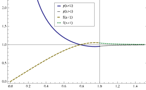
Figure 2 shows the behavior of $f_{\alpha}(x)$ and the corresponding $g_{\alpha}(x)=1/f_{\alpha}(x)$ and we see that they quickly tend to one beyond the scale $\sqrt{\gamma{\cal N}/2}\ell_{\rm P}$ , or the Planck length raised by the square root of the plaquette number ${\cal N}$ . Figure 3 shows the graphical solution of the horizon equation $M=x/2f_{\alpha}(x)$ for the example ${\cal N}=1$ and we see that there is a mass threshold below which no horizon forms. For other (constant) values of ${\cal N}$ the size of the mass threshold can easily be estimated as the limit

\lim_{x\to 0}\frac{x}{2f_{\alpha}(x)}=\frac{1}{4}e^{\pi/4-1/2}({\cal N}\gamma\ell_{\mathrm{P}}^{2}/2)^{1/4}\,.

(37)

Thus, for $M\lesssim\frac{1}{4}e^{\pi/4-1/2}{\cal N}^{1/4}\sim 0.33{\cal N}^{1/4}$ (in Planck units with $\gamma$ absorbed) no horizon forms. This observation agrees with results obtained independently with quantum corrections of inverse-triad type [35, 36, 28, 29]. For comparison we have also plotted the classical horizon curve and we see that the two curves are nearly indistinguishable beyond $x=\sqrt{\gamma{\cal N}/2}\ell_{\rm P}$ .

Given that small values of $x$ are associated with large curvature, the solutions are probably no longer reliable all the way down to $x=0$ ; other quantum corrections, ignored here, should be expected to become strong as well. However, since $x/f_{\alpha}(x)$ is monotonic, owing to ${\rm d}(x/f_{\alpha}(x))/{\rm d}x=\alpha(x)/f_{\alpha}(x)\geq 0$ , the limit (37) provides a lower bound for the threshold to which the ratio $M=x/2f_{\alpha}(x)$ asymptotes. Since the modified curve starts to deviate from the classical one at $x_{*}=\sqrt{\gamma{\cal N}/2}\ell_{\mathrm{P}}$ which for large ${\cal N}$ need not be deep inside the quantum regime, the limit, considered as an approximation for the asymptote value, gives a good estimate for the mass threshold.

Since the small- $x$ regime is likely to require all corrections, in addition to inverse-triad ones also quantum back-reaction and holonomy corrections (which, too, can be argued to lead to a mass threshold [37]), an analysis as the present one cannot provide hints for the full global structure or a conformal diagram.

Non-constant patch number:

If ${\cal N}$ is not constant but depends on $x$ , the correction functions $f_{\alpha}$ and $g_{\alpha}$ change. With a power-law ansatz ${\cal N}\propto x^{p}$ , the qualitative behavior of importance here does not strongly depend on $p$ , except in the interesting case $p=2$ in which the patch size (the orbit size divided by ${\cal N}$ ) is constant. We first present the formulas for general $p=:2+\epsilon$ , and then comment more specifically on $p=2$ or $\epsilon=0$ .

To be specific we choose a power-law behavior for the number of plaquettes i.e. $\mathcal{N}=b^{2}x^{2+\epsilon}$ . Here $b$ is a constant with dimesnsions $[L^{-(1+\epsilon/2)}]$ , introduced to ensure that $\mathcal{N}$ is dimensionless. From (8) we see that for the assumed form of $\mathcal{N}$ the correction function $\alpha$ becomes

\alpha=\frac{\sqrt{|1+a^{2}b^{2}x^{\epsilon}|}-\sqrt{|1-a^{2}b^{2}x^{\epsilon}|}}{a^{2}b^{2}x^{\epsilon}}\,,

(38)

where we have introduced the notation $a^{2}\equiv\gamma\ell_{\rm P}^{2}/2$ . We note that the point separating the deep quantum regime from the semiclassical regime is now dependent not just on the Planck scale through $a$ but also on the constant $b$ and the exponent $\epsilon$ .

It turns out that also for this form of $\alpha$ the differential equation (31) for $f_{\alpha}$ can be solved exactly. The solution is

f_{\alpha}(x)=c_{1}e^{\alpha/\epsilon}\left(1+\sqrt{1-a^{2}b^{2}x^{\epsilon}}\right)^{1/\epsilon}\left(1+\sqrt{1+a^{2}b^{2}x^{\epsilon}}\right)^{1/\epsilon}

(39)

for $1>a^{2}b^{2}x^{\epsilon}$ and

f_{\alpha}(x)=c_{2}x^{-1}\exp\left(\frac{\alpha}{\epsilon}+\frac{1}{2\epsilon}\arctan\left(\frac{-2+a^{2}b^{2}x^{\epsilon}}{2\sqrt{-1+a^{2}b^{2}x^{\epsilon}}}\right)\right)\left(1+\sqrt{1+a^{2}b^{2}x^{\epsilon}}\right)^{1/\epsilon}

(40)

for $1<a^{2}b^{2}x^{\epsilon}$ . The constants $c_{1}$ and $c_{2}$ are determined by imposing suitable boundary conditions. The condition $1>a^{2}b^{2}x^{\epsilon}$ , for which the solution in (39) has been written, would be valid for large $x$ only if $\epsilon<0$ . In this case $c_{1}$ is determined by requiring $f_{\alpha}(x)\rightarrow 1$ in the limit $x\rightarrow\infty$ , which gives $c_{1}=(4e)^{-1/\epsilon}$ . For $\epsilon=-2$ (and with $b=1$ ), which is the case considered previously, this correctly gives $c_{1}=2\sqrt{e}$ (see (35)). The constant $c_{2}$ is then determined by requiring continuity at $x^{\epsilon}=1/a^{2}b^{2}$ , which gives $c_{2}=(4e)^{-1/\epsilon}(ab)^{1/\epsilon}e^{\pi/4\epsilon}$ . For $\epsilon=-2$ , $c_{2}=2e^{1/2-\pi/8}/\sqrt{a}$ .

It is easy to see that for $\epsilon>0$ , the roles of the two solutions are reversed and it is the second solution above which will be valid for large values of $x$ . If we take the limit $x\rightarrow\infty$ in (40) with $\epsilon>0$ we find that it diverges, implying that we do not have the correct asymptotic limit. Another way to see this is to note that in this case $\alpha_{x\to\infty}\rightarrow 0$ whereas classically it should approach one. Thus we see that the case with $\epsilon>0$ does not correspond to physically acceptable solutions. Indeed, in this case the patch size $\Delta=E^{x}/{\cal N}$ shrinks as one moves out to larger radii, eventually falling into the regime where inverse-triad corrections are large.

We now consider the case $\epsilon=0$ (i.e. $\mathcal{N}\propto x^{2}$ ). In this case the correction function $\alpha$ turns out to be a constant:

\alpha=\frac{\sqrt{1+a^{2}b^{2}}-\sqrt{|1-a^{2}b^{2}|}}{a^{2}b^{2}}\,.

(41)

and the equation for $f_{\alpha}$ is solved by

f_{\alpha}(x)=c_{3}x^{1+a^{-2}b^{-2}\left(\sqrt{|1-a^{2}b^{2}|}-\sqrt{1+a^{2}b^{2}}\right)}\,.

(42)

In classical regimes, deviations of $\alpha$ from one should be small, and we are led to choose $a^{2}b^{2}\ll 1$ . This corresponds to an expression of $f_{\alpha}(x)$ proportional to $x$ raised to a very small negative power. Thus, although the function diverges at $x=0$ and goes to zero as $x\rightarrow\infty$ , for a large range of radii it is very nearly constant. Indeed, for $\mathcal{N}\propto x^{2}$ the size of plaquettes on every orbit is the same. Since inverse-triad corrections with refinement depend only on the plaquette size, they have the same value for all orbits and do not drop off as $x\to\infty$ . The only way to make the corrections small in any finite range of $x$ is then by choosing the proportionality constant $b^{2}$ in $\mathcal{N}=b^{2}x^{2}$ to be small, which is implied by the choice $a^{2}b^{2}\ll 1$ .

Nevertheless, the asymptotic structure of the full space-time is modified. First, one can check that the leading curvature invariants, the Ricci scalar, the Ricci tensor squared and the Riemann tensor squared, all vanish asymptotically. But asymptotic flatness is not obviously realized in the given slicing: In (34), the drop-off of $f_{\alpha}$ implies that the mass parameter $M$ plays no role for large $x$ , while the additional diverging factor of $g_{\alpha}(x)=1/f_{\alpha}(x)$ becomes relevant. For large $x$ , the metric turns out to be conformally related to the flat metric: For $g_{\alpha}(x)=g_{0}x^{\delta}$ with a small, positive $\delta$ , the line element for large $x$ is

{\rm d}s^{2}\sim-g_{\alpha}^{2}{\rm d}t^{2}+{\rm d}x^{2}+x^{2}{\rm d}\Omega^{2}=y^{2\delta/(1-\delta)}\left(-g_{0}^{2}{\rm d}t^{2}+(1-\delta)^{-2}{\rm d}y^{2}+y^{2}{\rm d}\Omega^{2}\right)

(43)

with $y:=x^{1-\delta}$ . However, the conformal factor diverges at $x\to\infty$ .

Thus, the simple-looking case of constant patch size (whose analog in isotropic quantum space-times is often used in cosmological models) implies non-trivial changes to the asymptotic form of the slicing used. Even though quantum corrections do not become larger as the asymptotic regime is approached, the cumulative effects of small corrections over a large range of radii add up and may lead to stronger effects in the asymptotic space-time. We leave a more detailed analysis for future work as the present article is mainly concerned with quasilocal horizon properties.

3.1.2 Modified Painlevé–Gullstrand metric

With the classical constraint algebra satisfied for the corrections with $\bar{\alpha}=1$ , we can look for a coordinate transformation to produce the Painlevé–Gullstrand form of the corrected metric (34). This coordinate system has as its time variable the proper time measured by a freely falling observer in the Schwarzschild spacetime (starting at rest from infinity and moving radially; see e.g. [38]). To determine this proper time we proceed as follows. The corrected Schwarzschild metric is independent of time and therefore $\xi_{(t)}=\partial_{t}$ is a Killing vector. Now consider the geodesic of a (radially) freely falling observer, with the tangent to the geodesic denoted by $u^{a}$ . Then we have $u_{a}\xi^{a}_{(t)}=E$ constant. If we parameterize the geodesic by its proper time $T$ and choose $E=-1$ , we have

g_{ab}u^{a}\xi^{b}_{(t)}=-\frac{1}{f_{\alpha}^{2}}\left(1-\frac{2Mf_{\alpha}}{x}\right)\frac{{\rm d}t}{{\rm d}T}=-1\,.

(44)

In addition, $g_{ab}u^{a}u^{b}=-1$ , or

-\frac{1}{f_{\alpha}^{2}}\left(1-\frac{2Mf_{\alpha}}{x}\right)\left(\frac{{\rm d}t}{{\rm d}T}\right)^{2}+\left(1-\frac{2Mf_{\alpha}}{x}\right)^{-1}\left(\frac{{\rm d}x}{{\rm d}T}\right)^{2}=-1

(45)

and with (44) we obtain

\frac{{\rm d}x}{{\rm d}T}=-\sqrt{f_{\alpha}^{2}-1+\frac{2Mf_{\alpha}}{x}}\,,

(46)

where the negative sign for the square root corresponds to an infalling observer. Thus, $u_{a}=(-1,-(1-2Mf_{\alpha}/x)^{-1}\sqrt{f_{\alpha}^{2}-1+2Mf_{\alpha}/x},0,0)$ and

{\rm d}T=-u_{a}{\rm d}x^{a}={\rm d}t+\left(1-\frac{2Mf_{\alpha}}{x}\right)^{-1}\sqrt{f_{\alpha}^{2}-1+\frac{2Mf_{\alpha}}{x}}{\rm d}x\,.

(47)

Inserting for ${\rm d}t$ from above in the Schwarzschild metric and simplifying we arrive at the metric in Painleve-Gullstrand-like coordinates

{\rm d}s^{2}=-\frac{1}{f_{\alpha}^{2}}\left(1-\frac{2Mf_{\alpha}}{x}\right){\rm d}T^{2}+f_{\alpha}^{-2}{\rm d}x^{2}+2f_{\alpha}^{-2}\sqrt{f_{\alpha}^{2}-1+\frac{2Mf_{\alpha}}{x}}{\rm d}T{\rm d}x+x^{2}{\rm d}\Omega^{2}\,.

(48)

(Notice that $T={\rm const}$ -slices, which are classically flat, are no longer so.)

In this derivation, we have made use of the fact that coordinate changes are gauge transformations for this type of corrections, and have used the usual geodesic properties in space-time. We can explicitly verify the first property by checking that the constraints are satisfied for the new form of the line element as well. By comparison with (3) we obtain $E^{x}=x^{2}$ and $E^{\varphi}=x/f_{\alpha}$ , as well as $N=1$ and $N^{x}=(f_{\alpha}^{2}-1+2Mf_{\alpha}/x)^{1/2}$ . These when used in (15) and the analogous equation for $K_{\varphi}$ , obtained from (22), give

K_{\varphi}=-\sqrt{f_{\alpha}^{2}-1+\frac{2Mf_{\alpha}}{x}}\quad,\quad K_{x}=\frac{\alpha f_{\alpha}+M\alpha/x-f_{\alpha}}{x\sqrt{f_{\alpha}^{2}-1+2Mf_{\alpha}/x}}\,.

(49)

The diffeomorphism constraint amounts to $2E^{\varphi}K_{\varphi}^{\prime}=K_{x}E^{x}{}^{\prime}$ which is satisfied, as is the Hamiltonian constraint. For later use, we note that $N=1$ appears to be a suitable way to specify the Painlevé–Gullstrand form without directly referring to space-time properties (while spatial flatness, as seen, can be violated by quantum corrections).

3.2 Space-time properties

For the uncorrected algebra, the usual space-time notions can be used to define and compute the position of horizons or other properties. In this section we first calculate the surface gravity and then give a detailed computation for the Hawking effect to show possible implications of space-time modifications.

To calculate the surface gravity we start by considering the 4-acceleration of a particle (of unit mass) held stationary at radius $x$ . For the case of a static, spherically symmetric metric the only non-zero component of the acceleration is $a^{x}=\Gamma^{x}_{tt}(u^{t})^{2}$ and the force required to hold the particle at radius $x$ by a local agent is $|a|=g_{xx}^{1/2}\Gamma^{x}_{tt}(u^{t})^{2}$ . The force required by an agent at infinity, defining surface gravity, differs by a red-shift factor of $g_{tt}^{1/2}$ , $\kappa=a_{\infty}(x)=g_{tt}^{1/2}|a|$ . At the horizon $x_{{\rm h}}=2Mf_{\alpha}$ , and the surface gravity is

\kappa|_{x_{{\rm h}}}=\left.\frac{\alpha}{4Mf_{\alpha}^{2}}\right|_{x_{{\rm h}}}\,.

(50)

For later use, we note that it can also be written as

\kappa=\frac{1}{2}\left.\frac{\partial C}{\partial x}\right|_{x=2Mf_{\alpha}}

(51)

with $C=g_{\alpha}(1-2Mf_{\alpha}/x)$ .

Since the solution is time independent we can go through the usual derivation of the Hawking effect [39, 40, 41]. We should note one crucial difference expected for a complete picture: as the black hole evaporates, its mass will decrease and will ultimately reach the limiting value below which the horizon disappears giving a naked singularity. In this regime, however, we can no longer consider our equations, or other corrections suggested by loop quantum gravity, reliable. (See [42, 43, 44, 45] for other calculations of horizons and evaporation with corrections motivated by loop quantum gravity.)

We start by rewriting the metric as

{\rm d}s^{2}=g_{\alpha}^{2}\left(1-\frac{2Mf_{\alpha}}{x}\right)\left[-{\rm d}t^{2}+\frac{{\rm d}x^{2}}{g_{\alpha}^{2}\left(1-2Mf_{\alpha}/x\right)^{2}}\right]+x^{2}{\rm d}\Omega^{2}\,.

(52)

Defining ${\rm d}x^{*}={\rm d}x/C={\rm d}x/g_{\alpha}\left(1-2Mf_{\alpha}/x\right)$ (with $C$ as above) and introducing the null coordinates $u=t-x^{*}+X_{0}^{*}$ , $v=t+x^{*}-X_{0}^{*}$ ( $X_{0}^{*}$ a constant), the metric becomes

{\rm d}s^{2}=\bar{C}(x){\rm d}u{\rm d}v

(53)

where $\bar{C}(x)=g_{\alpha}(x)C(x)=g_{\alpha}^{2}\left(1-2Mf_{\alpha}/x\right)$ . We now assume that this solution can be matched to a collapsing interior given by the metric

{\rm d}s^{2}=A(U,V){\rm d}U{\rm d}V

(54)

where $U=\tau-x+X_{0}$ and $V=\tau+x-X_{0}$ are the null coordinates in the interior with $x=X_{0}$ being the surface of the star at $\tau\leq 0$ . In general, the surface of the star is given by $x=X(\tau)$ . To simplify the calculations, in what follows, we will ignore the angular part of the metric and work in the 2-dimensional $(t,x)$ space. As is usually done, we restrict ourselves to the $x\geq 0$ region and impose the boundary condition that the scalar field $\chi$ vanishes at $x=0$ . In terms of the interior coodinates the line $x=0$ is given by

V=U-2X_{0}\,.

(55)

We now solve the 2-dimensional massless scalar wave equation $\Box\chi=0$ by functions that reduce to the standard form on $\mathcal{I}^{-}$ and are subject to the boundary condition $\chi=0$ along (55). If we let $U=a(u)$ and $v=b(V)$ denote the identification of coordinates between the interior and the exterior, then along $x=0$ we get

v=b(V)=b(U-2X_{0})=b(a(u)-2X_{0})\,.

This then gives the mode solution

\chi_{\rm in}=i(4\pi\omega)^{-1/2}(e^{-i\omega v}-e^{-i\omega b[a(u)-2X_{0}]})\,.

(56)

The complicated $u$ -dependence comes because the simple left-moving wave is converted, due to the exponential redshift suffered by the wave as the surface of the star approaches the horizon, to the complicated out-going wave by the collapsing star. To determine the free functions, we match the interior and the exterior metrics at the boundary $x=X(\tau)$ :

g_{\alpha}C\left(-{\rm d}t^{2}+\left(\frac{{\rm d}x}{C}\right)^{2}\right)=A(-{\rm d}\tau^{2}+{\rm d}x^{2})

such that

\dot{t}=\frac{\left(ACg_{\alpha}^{-1}(1-\dot{X}^{2})+\dot{X}^{2}\right)^{1/2}}{C}

where a dot here denotes derivative with respect to $\tau$ . Since $U=a(u)$ , taking the derivative of the two sides we obtain ${\rm d}U={\rm d}\tau(1-\dot{X})=a^{\prime}{\rm d}u=a^{\prime}(\dot{t}-\dot{X}/C){\rm d}\tau$ , or $a^{\prime}=C(1-\dot{X})/(C\dot{t}-\dot{X})$ . (In this section, a prime $(^{\prime})$ denotes derivative with respect to the argument of the function.) Inserting $\dot{t}$ ,

a^{\prime}=\frac{C(1-\dot{X})}{\left(ACg_{\alpha}^{-1}(1-\dot{X}^{2})+\dot{X}^{2}\right)^{1/2}-\dot{X}}\,.

(57)

The horizon is given by $C=0$ and therefore near the horizon, taking $(\dot{X}^{2})^{1/2}=-\dot{X}$ for a collapsing star, (57) simplifies to

a^{\prime}=\frac{C(\dot{X}-1)}{2\dot{X}}\,.

(58)

(Since $g_{\alpha}^{-1}=f_{\alpha}$ is bounded from above, the validity of neglecting the term involving $C$ is not affected by the presence of a factor of $1/g_{\alpha}$ .) Also, near $C=0$ we expand $X(\tau)$ as $X(\tau)=X_{{\rm h}}-\dot{X}(\tau_{{\rm h}})(\tau_{{\rm h}}-\tau)$ where the subscript ‘h’ designates the horizon. Using this we expand $C$ as

C(X)=C(X_{{\rm h}}-\dot{X}(\tau_{{\rm h}})(\tau_{{\rm h}}-\tau))=C(X_{{\rm h}})-\left.\frac{\partial C}{\partial x}\right|_{x_{{\rm h}}}\dot{X}(\tau_{{\rm h}})(\tau_{{\rm h}}-\tau)=-\left.\frac{\partial C}{\partial x}\right|_{x_{{\rm h}}}\dot{X}(\tau_{{\rm h}})(\tau_{{\rm h}}-\tau)\,.

Thus,

\frac{\partial{U}}{\partial{u}}=a^{\prime}=-(\dot{X}-1)(\tau_{{\rm h}}-\tau)\kappa

(59)

where $\kappa$ is given by (51). We thus have

-\kappa{\rm d}u=\frac{{\rm d}U}{(\dot{X}-1)(\tau_{{\rm h}}-\tau)}\,.

(60)

At the surface of the star, ${\rm d}U={\rm d}\tau(1-\dot{X})$ and therefore we get

-\kappa u=\ln|\tau-\tau_{{\rm h}}|+c_{1}=\ln|U+X_{{\rm h}}-X_{0}-\tau_{{\rm h}}|+c_{1}

(61)

where $c_{1}$ is a constant. Near $\tau\approx\tau_{{\rm h}}$ we therefore obtain

U=a(u)\propto e^{-\kappa u}+c_{2}

(62)

where $c_{2}$ is some constant. We note that due to the negative exponential, large changes in $u$ (the exterior coordinate at the surface) near the horizon, where $u$ is large, correspond to small changes in $U$ (the interior coordinate on the surface, near the horizon). Using similar arguments the function $b$ relating $v$ and $V$ , under the assumption $C\approx 0$ , is found to be

b^{\prime}=-\frac{A(1-\dot{X})}{2g_{\alpha}\dot{X}}\,.

(63)

Due to the presence of a horizon, all the null rays corresponding to $u=\rm constant$ near (and outside) the horizon, when traced back to $\mathcal{I}^{-}$ , correspond to a narrow range of $v=\rm constant$ rays. Similarly, because of the relation between $U$ and $V$ at the surface of the star, a narrow range of $U$ values corresponds to a narrow range in $V$ and therefore in the above equation one can assume $A(U,V)$ to be constant. In this limit we also assume that $g_{\alpha}$ is approximately a constant. (This assumption will not always be justified since depending on the mass and the lattice refinement scheme, the horizon could be at such a value of $x$ where $g_{\alpha}$ could be a rapidly varying function. Here, the possibility of stronger quantum effects arises which, however we will not explore in this paper.) The equation can then be integrated easily to give

v=-\frac{A(1-\dot{X})}{2g_{\alpha}\dot{X}}V+c_{3}\,.

(64)

Knowing the functions $a$ and $b$ we write the complicated phase factor in (56) as

\chi_{\rm in}=i(4\pi\omega)^{-1/2}(e^{-i\omega v}-e^{-i\omega[\bar{a}e^{-\kappa u}+\bar{b}]})\,.

(65)

Here $\bar{a}$ and $\bar{b}$ are some constants and as mentioned above, $g_{\alpha}$ has been taken to be a constant and absorbed with these two constants.

Instead of considering modes that are simple incoming waves on $\mathcal{I}^{-}$ and complicated outgoing waves as in the equation above, one may also consider modes which are simple outgoing waves on $\mathcal{I}^{+}$ but which (when traced back to $\mathcal{I}^{-}$ ) become complicated functions of $v$ . To do so, one has to invert the $u$ -dependent phase factor in (65) above. It is straightforward to see that this gives the following function of $v$

c(v)=-\frac{1}{\kappa}\ln\left|\frac{v-v_{0}}{\bar{a}}\right|

(66)

where $v_{0}$ corresponds to the latest value of $v$ such that the ray, starting on $\mathcal{I}^{-}$ , reaches $\mathcal{I}^{+}$ . This also implies $v_{0}>v$ . Thus this mode becomes

\chi_{\rm out}=i(4\pi\omega)^{-1/2}(e^{i\omega\kappa^{-1}\ln[(v_{0}-v)/\bar{a}]}-e^{-i\omega u})\,.

(67)

Knowing the ‘out’ mode on $\mathcal{I}^{-}$ , the next task is to calculate the Bogolubov coefficients relating the two sets of modes $\chi_{\rm in}$ and that portion of $\chi_{\rm out}$ that corresponds to waves going to $\mathcal{I}^{+}$ for $v<v_{0}$ , that is, $e^{-i\omega c(v)}$ . If the relation between the modes is given by

\chi_{\rm in}(\omega)=\int{\rm d}\omega^{\prime}\left(\alpha_{\omega\omega^{\prime}}\chi_{\rm out}(\omega^{\prime})+\beta_{\omega\omega^{\prime}}\chi^{*}_{\rm out}(\omega^{\prime})\right)\,,

(68)

then following the standard procedure, the relevant Bogolubov coefficient describing particle production is $\beta_{\omega\omega^{\prime}}$ . In terms of the standard inner product for scalar fields, this is given by $\beta_{\omega\omega^{\prime}}=-(\chi_{\rm in}(\omega),\chi_{\rm out}^{*}(\omega^{\prime}))$ . When evaluated this gives

|\beta_{\omega\omega^{\prime}}|^{2}=\frac{1}{2\pi\kappa\omega}\left(\frac{1}{e^{\omega^{\prime}/k_{\rm B}T-1}}\right)

(69)

with $T=\hbar\kappa/2\pi k_{\rm B}$ , $k_{\rm B}$ being the Boltzmann constant. Using $\kappa$ as given by (51) the temperature is

k_{\rm B}T=\frac{\hbar\alpha(x_{{\rm h}})g_{\alpha}^{2}(x_{{\rm h}})}{8\pi M}

(70)

where the horizon is given by $C=1-2Mf_{\alpha}/x_{\rm h}=0$ . In the limit $x\rightarrow\infty$ (for large $M$ ) we recover the well known result $k_{\rm B}T=\frac{\hbar}{8\pi M}$ .

The classical formulas are thus corrected by several factors from inverse-triad corrections. But there was also an additional position-dependence in the derivation, which, in regimes where it must be taken into account, makes the analysis more complicated but might introduce new and stronger effects.

4 Second-order perturbations

We now perform perturbative calculations for the classical vacuum constraints, to be used in the context of matter back-reaction. Although the classical vacuum constraints can be solved exactly, the perturbative procedure as well as some of the equations will be useful later. We will also take this opportunity to state our background gauge conditions for the two versions of the space-time, Schwarzschild and Painlevé–Gullstrand. For each of the backgrounds considered, we will perform the following steps:

Step 1: 1st-order perturbation of the Hamiltonian and diffeomorphism constraints.
Step 2: 1st-order perturbation of the equations of motion.
Step 3: 2nd-order perturbation of constraints including matter fields.
Step 4: 2nd-order perturbation of the equations of motion, as necessary.
Step 5: Calculation of the perturbed form of the metric and evaluation of horizon conditions to find area-mass relationships.

In addition, the following features are common to all the calculations:

•

The perturbations of the fundamental variables ( $E^{x},E^{\varphi},K_{x},K_{\varphi}$ ) will be denoted as:

$E^{\varphi}\rightarrow E^{\varphi}+\Delta E^{\varphi}=E^{\varphi}+\,\delta\!E^{\varphi}+\delta_{2}E^{\varphi}$ (71)

and so on. In every case, a $\delta$ without a subscript is to be taken to refer to a first-order perturbation of the relevant quantity. Fields without any kind of delta refer to the background values.
•

Since we are interested in possible changes to the area of various surfaces, we will, for simplicity of calculation, make the gauge choice

$E^{x}=x^{2}$ (72)

to fix the diffeomorphism constraint. In particular, we set $\Delta E^{x}=0$ , and the perturbation of $E^{x}$ at every order is set to zero. We will not be fixing the gauge completely. Rather, the presence of gauge-dependent terms (under transformations generated by the perturbed Hamiltonian constraint) will be taken as one of the criteria to distinguish between the horizon conditions used in various models with different types of inverse-triad corrections. A key consistency requirement will be that horizon conditions be gauge invariant.
•

We consider the matter field and its corresponding conjugate momentum to be first order perturbations (the background space-time is vacuum), which implies that the energy density $\rho$ and the energy-momentum flux $J^{x}$ are to be included only in the second order and higher perturbations of the constraints.

The different slicings (Schwarzschild and Painlevé–Gullstrand) are implemented by specifying the background fields. We will carry out the steps of the calculation in detail for the Painlevé–Gullstrand metric for an uncharged non-rotating black hole. For subsequent calculations we will only list the relevant changes. First, we provide two canonical versions of horizon conditions to be used.

4.1 Horizon conditions

We define horizons in canonical variables in order to be able to apply them to equations corrected by effects from canonical quantum gravity. For comparison, we provide two versions which would classically be equivalent in the context of spherically symmetric geometries. In doing so, we must use space-time notions to capture the meaning of a horizon, and it is not guaranteed that such definitions are reasonable for models with a deformed constraint algebra and their new versions of space-time structures. The motivation for providing two versions of horizon conditions is that we can test whether they remain equivalent in the deformed context and then have a chance of capturing the same effects. For cases with an uncorrected constraint algebra, we will furthermore compare with the direct space-time analysis.

4.1.1 Trapping horizon

Horizons of our perturbative solutions can be analyzed by an expansion of the usual conditions, for instance of [46]. In spherical symmetry, the cross-section of a spatial slice with a spherical trapping horizon as the boundary of spherical marginally trapped surfaces, can be defined simply as a sphere at radius $x$ whose co-normal $\mathrm{d}x_{a}$ is null. This condition may be written as $g^{xx}=0$ ; one can verify that zero expansion of null geodesics is then implied. In triad variables with line element (3) one obtains the condition

\frac{E^{x}}{(E^{\varphi})^{2}}-\left(\frac{N^{x}}{N}\right)^{2}=0

(73)

which can easily be analyzed perturbatively. To second order in the perturbations, it expands to:

\begin{split}&\bigg[\frac{E^{x}}{(E^{\varphi})^{2}}-\left(\frac{N^{x}}{N}\right)^{2}\bigg]_{0}\\ &+\bigg[-2\frac{E^{x}\,\delta\!E^{\varphi}}{(E^{\varphi})^{3}}-2\frac{N^{x}\,\delta\!N^{x}}{N^{2}}+2\frac{(N^{x})^{2}\delta\!N}{N^{3}}\bigg]_{1}\\ &+\bigg[-2\frac{E^{x}\delta_{2}E^{\varphi}}{(E^{\varphi})^{3}}-2\frac{N^{x}\,\delta_{2}\!N^{x}}{N^{2}}+2\frac{(N^{x})^{2}\delta_{2}\!N}{N^{3}}+3\frac{E^{x}(\,\delta\!E^{\varphi})^{2}}{(E^{\varphi})^{4}}\\ &-\frac{(\,\delta\!N^{x})^{2}}{N^{2}}-3\frac{(N^{x}\delta\!N)^{2}}{N^{4}}+4\frac{N^{x}\,\delta\!N^{x}\delta\!N}{N^{3}}\bigg]_{2}=0\,.\end{split}

(74)

4.1.2 Isolated horizon

Alternatively, for the Schwarzschild slicing we can define a spherical horizon by using the specialization of isolated horizon conditions [47] to spherical symmetry. Since matter is still allowed outside the horizon, a situation comparable to the previous definition is obtained, but the condition is more restrictive because no matter is allowed at the horizon.

We are now dealing with the condition [48]

A_{\varphi}=\sqrt{K_{\varphi}^{2}+\Gamma_{\varphi}^{2}}=0\,.

(75)

In the Schwarzschild metric this gives us two conditions:

K_{\varphi}^{2}=0\quad\mbox{and thus}\quad\,\delta\!K_{\varphi}^{2}=0

(76)

and

\Gamma_{\varphi}^{2}=0\quad\mbox{or}\quad\Gamma_{\varphi}^{2}+2\Gamma_{\varphi}\delta\Gamma_{\varphi}+2\Gamma_{\varphi}\delta_{2}\Gamma_{\varphi}+(\delta\Gamma_{\varphi})^{2}=0\,.

(77)

The fact that we have two conditions instead of just one as in (74) demonstrates the more restrictive notion. In spherical symmetry, it turns out that the difference does not matter much classically, but it will become important with spacetime-deforming quantum corrections.

4.1.3 Comparison and gauge

The origin of the additional condition arising for isolated horizons can be seen in the fact that isolated horizons, defined as boundaries of space-time, freeze gauge transformations generated by the Hamiltonian constraint on the horizon by boundary conditions. The additional condition on $K_{\varphi}$ then formally replaces a possible gauge-fixing condition one might choose in a treatment where the horizon is not a boundary. Classically, the trapping-horizon condition (74) is gauge invariant, and its evaluation does not depend on which gauge fixing is used. It thus implies results equivalent to those produced by the isolated-horizon condition.

However, it turns out that the condition (74) is no longer gauge invariant for some versions of quantum corrected constraints. The horizon condition itself will then have to be corrected so as to cancel the gauge dependence, thereby shedding some light on what quantum horizon conditions could look like. For an isolated horizon, on the other hand, having the Hamiltonian gauge fixed by boundary conditions eliminates the important option of seeing how horizon conditions must be corrected in addition to the dynamics of quantum gravity. We will address these questions in detail by the examples provided in the rest of this article.

4.2 Painlevé–Gullstrand

The Painlevé–Gullstrand form of the Schwarzschild space-time is

{\rm d}s^{2}=-\left(1-\frac{2M}{x}\right){\rm d}t^{2}+{\rm d}x^{2}+2\sqrt{\frac{2M}{x}}{\rm d}t{\rm d}x+x^{2}{\rm d}\Omega^{2}\,.

(78)

It is characterized by several interesting properties, such as having flat spatial slices of constant $t$ . In what follows, the background solutions will appear as coefficients of perturbation equations, partially identifying the gauge in which perturbations are analyzed. For the Painlevé–Gullstrand background,

E^{\varphi}=x,\quad N=1,\quad N^{x}=\sqrt{\frac{2M}{x}},\quad K_{x}=\sqrt{\frac{M}{2x^{3}}},\quad\text{and}\quad K_{\varphi}=-\sqrt{\frac{2M}{x}}

in addition to (72).

4.2.1 First order perturbation of the constraints

We expand the Hamiltonian and diffeomorphism constraint equations $\delta\mathbf{H}[N]/\delta N=0$ and $\delta\mathbf{D}[N^{x}]/\delta N^{x}=0$ to first order in metric perturbations, obtaining the general forms

	$\displaystyle 2($	$\displaystyle K_{\varphi}E^{\varphi}+K_{x}E^{x})\,\delta\!K_{\varphi}+2K_{\varphi}E^{x}\,\delta\!K_{x}+(K_{\varphi}^{2}-\Gamma_{\varphi}^{2}+1)\,\delta\!E^{\varphi}$
		$\displaystyle+2(K_{\varphi}K_{x}+\Gamma_{\varphi}^{\prime})\,\delta\!E^{x}-2\Gamma_{\varphi}E^{\varphi}\delta\Gamma_{\varphi}+2E^{x}\delta\Gamma_{\varphi}^{\prime}=0$		(79)

and

2E^{\varphi}\,\delta\!K_{\varphi}^{\prime}+2K_{\varphi}^{\prime}\,\delta\!E^{\varphi}-K_{x}\,\delta\!E^{x^{\prime}}-E^{x^{\prime}}\,\delta\!K_{x}=0

(80)

Inserting the unperturbed form of the densitized triad and extrinsic curvature corresponding to (78), and applying the gauge condition $\,\delta\!E^{x}=0$ , with the additional corollaries that $\,\delta\!E^{x^{\prime}}=0$ and $\delta\Gamma_{\varphi}=\frac{E^{x}\,{}^{\prime}}{2E^{\varphi}\,{}^{2}}\delta E^{\varphi}$ , we have:

-\sqrt{2Mx}\,\delta\!K_{\varphi}-2\sqrt{2Mx^{3}}\,\delta\!K_{x}+\frac{2M}{x}\,\delta\!E^{\varphi}+2x\,\delta\!E^{\varphi^{\prime}}=0

(81)

and

2\sqrt{2Mx}\,\delta\!K^{\prime}_{\varphi}+\frac{2M}{x^{2}}\,\delta\!E^{\varphi}-2\sqrt{2Mx}\,\delta\!K_{x}=0\,.

(82)

To proceed solving the equations as far as possible, we subtract (81) and (82) to obtain

\,\delta\!E^{\varphi^{\prime}}=\frac{1}{2}\sqrt{\frac{2M}{x}}\,\delta\!K_{\varphi}+\sqrt{2Mx}\,\delta\!K^{\prime}_{\varphi}=(\sqrt{2Mx}\,\,\delta\!K_{\varphi})^{\prime}\,,

(83)

which can immediately be integrated. If we impose the boundary conditions that all the perturbations fall off to zero at infinity, and in particular, that

\sqrt{x}\,\delta\!K_{\varphi}\rightarrow 0\quad\mbox{as}\quad x\rightarrow\infty\,,

(84)

this equation can be solved by

\,\delta\!E^{\varphi}=\sqrt{2Mx}\,\delta\!K_{\varphi}\,,

(85)

and, substituting this back in (82)

\,\delta\!K_{x}=\frac{M}{x^{2}}\,\delta\!K_{\varphi}+\,\delta\!K^{\prime}_{\varphi}\,.

(86)

4.2.2 Perturbation of the Equations of motion

We obtain the linear equations of motion by expanding the general spherically symmetric equations (22)–(27) with $\bar{\alpha}=\alpha=1$ . Equation (22) gives to first order

\delta\dot{E}^{x}=2|E^{x}|^{\frac{1}{2}}(K_{\varphi}\delta\!N+N\,\delta\!K_{\varphi})+NK_{\varphi}|E^{x}|^{-\frac{1}{2}}\,\delta\!E^{x}+N^{x}\,\delta\!E^{x^{\prime}}+E^{x^{\prime}}\,\delta\!N^{x}

(87)

\delta\dot{E}^{x}=-2x\sqrt{\frac{2M}{x}}\delta\!N+2x\,\delta\!K_{\varphi}-\frac{1}{x}\sqrt{\frac{2M}{x}}\,\delta\!E^{x}+\sqrt{\frac{2M}{x}}\,\delta\!E^{x^{\prime}}+2x\,\delta\!N^{x}

(88)

with the background solution (78) inserted for the unperturbed variables. We have $\delta\dot{E}^{\varphi}=\sqrt{2Mx}\delta\dot{K}_{\varphi}$ from (85). Using the equations of motion, this provides a second relation between $\delta N$ , $\delta K_{\varphi}$ and $\delta N^{x}$ which turns out to be identically satisfied.

To implement the gauge for the perturbations, we set $\,\delta\!E^{x}$ and all its derivatives to zero, to give:

-\sqrt{\frac{2M}{x}}\,\delta\!N+\,\delta\!K_{\varphi}+\,\delta\!N^{x}=0\,.

(89)

If we make the further choice that $\,\delta\!N=0$ , we can use the relations derived above to arrive at simplified equations for the other perturbations; in particular $\delta N^{x}=-\delta K_{\varphi}$ and:

\dot{\,\delta\!K_{\varphi}}=\sqrt{\frac{2M}{x}}\,\delta\!K^{\prime}_{\varphi}-\frac{1}{2x}\sqrt{\frac{2M}{x}}\,\delta\!K_{\varphi}\,.

(90)

The first order set of equations is solved by the general solution to (90):

\delta K_{\varphi}=\sqrt{x}\,F\left(2x^{3/2}/3+\sqrt{2M}\,t\right)

for an arbitrary function $F$ of one variable as indicated, satisfying the asymptotic condition (84). However, this extra gauge condition $\,\delta\!N=0$ is not necessary for our later results. The expressions for $\,\delta\!K_{x}$ , $\,\delta\!E^{\varphi}$ and $\,\delta\!N^{x}$ in terms of $\,\delta\!K_{\varphi}$ are consistent, and satisfy equations (26) and (27) for $\dot{\,\delta\!K_{\varphi}}$ and $\dot{\,\delta\!K_{x}}$ .

4.2.3 Second order perturbation of the constraints including matter

The second-order diffeomorphism constraint including matter is

2\delta E^{\varphi}\delta K_{\varphi}^{\prime}+2E^{\varphi}\delta_{2}K_{\varphi}^{\prime}+2K_{\varphi}^{\prime}\delta_{2}E^{\varphi}-E^{x}\,{}^{\prime}\delta_{2}K_{x}-8\pi E^{\varphi}|E^{x}|^{\frac{1}{2}}J_{x}=0\,,

(91)

so in our coordinates and using first order results we have

4M\,\delta\!K_{\varphi}\,\delta\!K^{\prime}_{\varphi}+2\sqrt{2Mx}\,\delta_{2}K^{\prime}_{\varphi}+\frac{2M}{x^{2}}\delta_{2}E^{\varphi}-2\sqrt{2Mx}\,\delta_{2}K_{x}-8\pi x^{2}\sqrt{\frac{2M}{x}}J_{x}=0\,.

(92)

The second-order Hamiltonian constraint

$\displaystyle($	$\displaystyle K_{\varphi}^{2}-\Gamma_{\varphi}^{2}+1)\delta_{2}E^{\varphi}+2K_{\varphi}E^{x}\delta_{2}K_{x}+2(K_{\varphi}E^{\varphi}+K_{x}E^{x})\delta_{2}K_{\varphi}$
	$\displaystyle-2\Gamma_{\varphi}E^{\varphi}\delta_{2}\Gamma_{\varphi}+2E^{x}\delta_{2}\Gamma_{\varphi}^{\prime}+2K_{\varphi}\delta K_{\varphi}\delta E^{\varphi}+E^{\varphi}(\delta K_{\varphi})^{2}$
$\displaystyle+$	$\displaystyle 2E^{x}\delta K_{\varphi}\delta K_{x}-2\Gamma_{\varphi}\delta\Gamma_{\varphi}\delta E^{\varphi}-E^{\varphi}(\delta\Gamma_{\varphi})^{2}-8\pi E^{\varphi}\|E^{x}\|\rho=0$	(93)

with $\delta_{2}\Gamma_{\varphi}=\frac{E^{x}\,{}^{\prime}}{2E^{\varphi}\,{}^{2}}\delta_{2}E^{\varphi}-\frac{E^{x}\,{}^{\prime}}{2E^{\varphi}\,{}^{3}}(\delta E^{\varphi})^{2}$ , requires a little more work and gives

\begin{split}&-\sqrt{\frac{2M}{x}}\delta_{2}K_{\varphi}-\sqrt{8Mx}\delta_{2}K_{x}+\frac{2M}{x^{2}}\delta_{2}E^{\varphi}+2\delta_{2}E^{\varphi^{\prime}}+\bigg((x-4M)(\,\delta\!K_{\varphi})^{2}\bigg)^{\prime}-8\pi x^{2}\rho=0\,,\end{split}

(94)

Subtracting these constraints,

2\delta_{2}E^{\varphi^{\prime}}=\sqrt{\frac{2M}{x}}\delta_{2}K_{\varphi}+2\sqrt{2Mx}\,\delta_{2}K^{\prime}_{\varphi}-((x-6M)(\,\delta\!K_{\varphi})^{2})^{\prime}+8\pi x^{2}\mathcal{H}

(95)

and integrating gives

\delta_{2}E^{\varphi}=\sqrt{2Mx}\delta_{2}K_{\varphi}-\frac{1}{2}(x-6M)(\,\delta\!K_{\varphi})^{2}-\frac{1}{2}\int_{x}^{\infty}\mathrm{d}z\>8\pi z^{2}\mathcal{H}

(96)

where we have used

\mathcal{H}:=N\rho-N^{x}J_{x}\,.

(97)

4.2.4 Second order perturbation of the equations of motion

We may proceed putting (96) back into the diffeomorphism constraint (92) to get an equation for $K_{x}$ in terms of $K_{\varphi}$ . Equation (22) gives

-\sqrt{\frac{2M}{x}}\delta_{2}N+\delta_{2}K_{\varphi}+\delta_{2}N^{x}+\delta N\delta K_{\varphi}=0

(98)

and (23), upon using these and the first order equations, results in an evolution equation for $K_{\varphi}$ consistent with equation (26). Since we will not use these equations for the horizon conditions we will not write them here.

4.2.5 Perturbation of the metric and horizon

After inserting the relevant expressions into (74), we find that the zeroth order terms are naturally the same as for the background, the first order terms vanish — which is to be expected since the matter terms have not yet played a part — and the second order terms include an influence from the matter fields. The condition on the horizon becomes:

1-\frac{2M}{x}+\frac{2}{x}\int_{x}^{\infty}\mathrm{d}z\>4\pi z^{2}\mathcal{H}=0

(99)

which tells us that

R_{\rm hor}=2\bigg(M-\int_{R_{\rm hor}}^{\infty}\mathrm{d}z\>4\pi z^{2}\mathcal{H}\>\bigg)\,.

(100)

The horizon radius is simply shifted from the vacuum value $2M$ in terms of the asymptotic mass by the amount of energy contributed by matter between the horizon and spatial infinity. The dependence on $\Delta K_{\varphi}$ in some solutions, for instance in (96), automatically cancels when they are combined to the horizon condition: the resulting condition is gauge invariant.

4.3 Schwarzschild

We proceed with the calculations in the Schwarzschild metric in a manner analogous to the Painlevé–Gullstrand case.

4.3.1 Step 1

In the Schwarzschild metric, assuming $\,\delta\!E^{x}=0$ , the first order Hamiltonian constraint (79) can be simplified to

\bigg(2\bigg(1-\frac{2M}{x}\bigg)^{3/2}\,\delta\!E^{\varphi}\bigg)^{\prime}=0\,.

(101)

The simplest solution to satisfy this constraint is to have $\,\delta\!E^{\varphi}=c(1-2M/x)^{-3/2}$ . However this choice blows up near the horizon faster than $E^{\varphi}=x(1-2M/x)^{-1/2}$ , so we make the choice $\,\delta\!E^{\varphi}=0$ .

In the Schwarzschild gauge, the first order diffeomorphism constraint (80) becomes

\,\delta\!K^{\prime}_{\varphi}=\sqrt{1-\frac{2M}{x}}\,\delta\!K_{x}\,.

(102)

This relation will be used repeatedly to simplify the second order constraints and equations of motion.

4.3.2 Step 2

¿From the first order perturbation of equation (22) for $E^{x}$ we derive

\,\delta\!N^{x}=-\sqrt{1-\frac{2M}{x}}\,\delta\!K_{\varphi}\,.

(103)

Considering (23), the equation of motion for $E^{\varphi}$ , we find:

\dot{\,\delta\!E^{\varphi}}=\,\delta\!K_{\varphi}+x\sqrt{1-\frac{2M}{x}}\,\delta\!K_{x}+\bigg(x\bigg(1-\frac{2M}{x}\bigg)^{-1/2}\,\delta\!N^{x}\bigg)^{\prime}

which, using (102) and (103), simplifies to

\dot{\,\delta\!E^{\varphi}}=\,\delta\!K_{\varphi}+x\,\delta\!K^{\prime}_{\varphi}+(-x\,\delta\!K_{\varphi})^{\prime}=0

(104)

and ensures that $\,\delta\!E^{\varphi}$ remains zero.

Finally, equation (26) gives the additional relation

\delta\dot{K_{\varphi}}=\left(1-\frac{2M}{x}\right)\delta N^{\prime}-\frac{M}{x^{2}}\delta N

(105)

4.3.3 Step 3

The second order Hamiltonian constraint (93), after simplification and discarding terms containing $\,\delta\!E^{\varphi}$ , becomes

\bigg(2\bigg(1-\frac{2M}{x}\bigg)^{3/2}\delta_{2}E^{\varphi}\bigg)^{\prime}+\bigg(x(\,\delta\!K_{\varphi})^{2}\bigg)^{\prime}-8\pi x^{2}\rho=0

(106)

and implies

2\bigg(1-\frac{2M}{x}\bigg)^{3/2}\delta_{2}E^{\varphi}+x(\,\delta\!K_{\varphi})^{2}=-\int_{x}^{\infty}\mathrm{d}z\>{8\pi z^{2}\rho}\,.

(107)

The relation provided by the diffeomorphism constraint (91) and the second order equations of motion are not needed here to derive the horizon condition, so we may proceed directly to step 5.

4.3.4 Step 5

The condition on the horizon is:

1-\frac{2M}{x}+\frac{2}{x}\int_{x}^{\infty}\mathrm{d}z\>4\pi z^{2}\mathcal{H}=0

(108)

where in the Schwarzschild slicing $\mathcal{H}=\rho$ . This agrees with our Painlevé–Gullstrand result.

Additionally, we can use the isolated horizon conditions, and we find that (77) gives, after setting $\,\delta\!E^{\varphi}=0$ :

1-\frac{2M}{x}+\,\delta\!K_{\varphi}^{2}-\frac{2}{x}\bigg(1-\frac{2M}{x}\bigg)^{3/2}\delta_{2}E^{\varphi}=0\,.

(109)

But since $\,\delta\!K_{\varphi}^{2}=0$ from (76) at the isolated horizon, we once again have:

1-\frac{2M}{x}+\frac{2}{x}\int_{x}^{\infty}{\mathrm{d}z\,4\pi z^{2}\rho}=0\,.

(110)

showing that we get equivalent results for the two methods of deriving the position of the horizon.

5 Inverse-triad corrections

We are especially interested in horizon conditions in the presence of back-reaction and quantum corrections. For $\bar{\alpha}=1$ the constraints satisfy the classical hypersurface-deformation algebra despite the presence of corrections. Effective line elements can thus be used to describe the space-time geometry and standard horizon definitions are applicable. We will first evaluate these definitions in the presence of corrections, which still provide equivalent results. This outcome is non-trivial since the modified dynamics could have led to stronger changes of the horizon behavior, rendering different definitions inequivalent. Moreover, the results of horizon conditions will be gauge invariant.

For $\alpha=\bar{\alpha}\not=1$ we have a modified constraint algebra but can obtain horizon formulas simply by substitution after absorbing $\alpha$ in the lapse function as far as the gravitational part of the Hamiltonian constraint is concerned. (There are still non-trivial quantum corrections: Matter Hamiltonians are non-classical even if we absorb $\alpha$ in the lapse function for the gravitational part, unless $U=0$ and $\nu=\sigma=\alpha$ in (18).)

The most interesting case is thus that of $1\not=\bar{\alpha}\not=\alpha$ , which as stated previously can be related to these two special cases. Here, the standard horizon conditions will no longer be gauge invariant, but we present a modification leading to satisfactory results. We will come back to conclusions drawn from this case in the discussions.

5.1 Classical algebra

Modified dynamics in the presence of ordinary space-time structure can directly be evaluated by the canonical horizon definitions.

5.1.1 Modified Painlevé–Gullstrand gauge

We consider the modified Painlevé–Gullstrand metric (48) as our background. The correction function $\alpha$ depends only on $E^{x}$ , so by assuming $\,\delta\!E^{x}=0$ , we also have $\delta\alpha=0$ . We will use the short hand notation:

h:=f_{\alpha}^{2}-1+\frac{2Mf_{\alpha}}{x}\,.

(111)

Step 1

Modified Hamiltonian constraint H[N]:

To first order, assuming $\,\delta\!E^{x}=0$ , the modified Hamiltonian constraint reads

\begin{split}2(\alpha K_{\varphi}E^{\varphi}+&K_{x}E^{x})\,\delta\!K_{\varphi}+2K_{\varphi}E^{x}\,\delta\!K_{x}+\alpha(K_{\varphi}^{2}-\Gamma_{\varphi}^{2}+1)\,\delta\!E^{\varphi}\\ &-2\alpha\Gamma_{\varphi}E^{\varphi}\delta\Gamma_{\varphi}+2E^{x}\delta\Gamma_{\varphi}^{\prime}=0\,.\end{split}

(112)

For the modified Painlevé–Gullstrand metric, using the relation between $\alpha$ and $f_{\alpha}$ , this simplifies to:

\bigg(\frac{x\sqrt{h}}{f_{\alpha}}\bigg)^{\prime}\,\delta\!K_{\varphi}+x\sqrt{h}\,\delta\!K_{x}-\frac{f_{\alpha}^{2}}{x}(x\,\delta\!E^{\varphi})^{\prime}+\frac{f_{\alpha}}{x}\bigg(\frac{x}{f_{\alpha}}\bigg)^{\prime}\bigg(\frac{-Mf_{\alpha}}{x}+f_{\alpha}^{2}\bigg)\,\delta\!E^{\varphi}=0\,.

(113)

Diffeomorphism constraint $D[N^{x}]$ :

Equation (80) becomes:

\frac{x\sqrt{h}}{f_{\alpha}}\,\delta\!K^{\prime}_{\varphi}-\sqrt{h}(\sqrt{h})^{\prime}\,\delta\!E^{\varphi}-x\sqrt{h}\,\delta\!K_{x}=0\,.

(114)

Adding these first order equations, we get an expression that simplifies to:

\bigg(\frac{x\sqrt{h}}{f_{\alpha}}\,\delta\!K_{\varphi}\bigg)^{\prime}-(f_{\alpha}^{2}\,\delta\!E^{\varphi})^{\prime}=0

(115)

which implies, with the appropriate fall off conditions at infinity, that

\,\delta\!E^{\varphi}=\frac{x\sqrt{h}}{f_{\alpha}^{3}}\,\delta\!K_{\varphi}\,.

(116)

Step 2

The equation of motion (22) for $E^{x}$ gives us the relation

-\sqrt{h}\,\delta\!N+\,\delta\!K_{\varphi}+\,\delta\!N^{x}=0

(117)

in this modified Painlevé–Gullstrand metric.

Step 4

Similarly for the second order perturbation of the same equation, we derive

\,\delta\!N\,\delta\!K_{\varphi}-\sqrt{h}\,\delta_{2}N+\delta_{2}K_{\varphi}+\delta_{2}N^{x}=0\,.

(118)

Step 3

Adding the second order constraints, integrating and rearranging, we get

\frac{2x\sqrt{h}}{f_{\alpha}}\delta_{2}K_{\varphi}-\bigg(\frac{x}{f_{\alpha}}-\frac{3xh}{f_{\alpha}^{3}}\bigg)(\,\delta\!K_{\varphi})^{2}-2f_{\alpha}^{2}\delta_{2}E^{\varphi}=\int_{x}^{\infty}\mathrm{d}z\>8\pi z^{2}\frac{\mathcal{H}}{f_{\alpha}}

(119)

where

\mathcal{H}=N{\rho}-N^{x}J_{x}\,.

(120)

Step 5

The condition on the horizon in the modified metric is:

1-\frac{2Mf_{\alpha}}{x}+\frac{2f_{\alpha}}{x}\int_{x}^{\infty}{\mathrm{d}z\>\,4\pi z^{2}\frac{\mathcal{H}}{f_{\alpha}}}=0

(121)

which agrees with the classical Painlevé–Gullstrand result in the limit that $f_{\alpha}\rightarrow 1$ . Gauge-dependent terms such as $\delta K_{\varphi}$ drop out and there is no need to fix the Hamiltonian gauge.

5.1.2 Modified Schwarzschild gauge

Step 1

Modified Hamiltonian constraint $H[N]$ :

Using the relation between $\alpha$ and $f_{\alpha}$ , equation (112) simplifies to:

\bigg(\frac{2}{f_{\alpha}}\bigg(1-\frac{2Mf_{\alpha}}{x}\bigg)^{3/2}\,\delta\!E^{\varphi}\bigg)^{\prime}=0\,.

(122)

The simplest solution to satisfy this constraint is to have $\,\delta\!E^{\varphi}=0$ .

Diffeomorphism constraint $D[N^{x}]$ :

Equation (80) for this metric gives the relation:

\,\delta\!K^{\prime}_{\varphi}=\sqrt{1-\frac{2Mf_{\alpha}}{x}}\,\delta\!K_{x}\,.

(123)

Step 2

From the first order perturbation of the equation of motion for $E^{x}$ , we have:

\,\delta\!N^{x}=-\frac{\,\delta\!K_{\varphi}}{f_{\alpha}}\sqrt{1-\frac{2Mf_{\alpha}}{x}}\,.

(124)

For the equation of motion of $\,\delta\!E^{\varphi}$ , we find

\dot{\,\delta\!E^{\varphi}}=\bigg(-\frac{x}{f_{\alpha}}\,\delta\!K_{\varphi}\bigg)^{\prime}+\frac{x}{f_{\alpha}}(\,\delta\!K_{\varphi})^{\prime}+\bigg(\frac{1}{f_{\alpha}}-\frac{xf_{\alpha}^{\prime}}{f_{\alpha}^{2}}\bigg)\,\delta\!K_{\varphi}=0

(125)

which, once again, ensures that $\,\delta\!E^{\varphi}$ remains zero.

Step 3

The second order Hamiltonian constraint, after simplification and discarding terms which contain $\,\delta\!E^{\varphi}$ , becomes:

\bigg(\frac{2}{f_{\alpha}}\bigg(1-\frac{2Mf_{\alpha}}{x}\bigg)^{3/2}\delta_{2}E^{\varphi}\bigg)^{\prime}+\bigg(\frac{x(\,\delta\!K_{\varphi})^{2}}{f_{\alpha}}\bigg)^{\prime}-\frac{8\pi x^{2}\rho}{f_{\alpha}}=0\,,

(126)

As in the classical Schwarzschild case, the relations from the second order diffeomorphism constraint (91) and equations of motion are not needed to derive the expression for the horizon condition.

For the horizon condition, we arrive at

1-\frac{2Mf_{\alpha}}{x}+\frac{2f_{\alpha}}{x}\int_{x}^{\infty}{\mathrm{d}z\;4\pi z^{2}\frac{\rho}{f_{\alpha}}}=0

(127)

which agrees with the classical Schwarzschild result in the limit that $f_{\alpha}\rightarrow 1$ . Equivalent results, (121) and (127) are obtained with both slicings and, in the Schwarzschild slicing, with both definitions of horizons. Moreover, for vacuum the result is in agreement with the direct space-time analysis performed in Sec. 3, which applies in this subsection where the classical algebra is assumed in the presence of corrections. In both cases, $\delta K_{\varphi}$ -terms automatically cancel in the horizon equation.

5.2 Modified algebra, absorbable

Before we evaluate horizon conditions in the case of a modified constraint algebra, we present calculations that show the overall consistency of the equations of motion and constraints. We will perform some of the calculations explicitly for the choice $N\alpha=1$ with a scalar matter field, illustrating how the anomaly-freedom condition is necessary to obtain consistent equations. (See the Appendix for an illustration of the inconsistency of line elements in this case with modified space-time structures.)

5.2.1 Dynamical consistency

First-order equations and results for this case are identical to those in sections 4.2.1 and 4.2.2. The second-order diffeomorphism constraint is the same as (92), and in the second order Hamiltonian constraint (94) the matter term is replaced by $-2x\alpha^{-1}(\nu\tilde{\mathcal{H}}_{\pi}+\sigma\tilde{\mathcal{H}}_{\nabla}+\tilde{\mathcal{H}}_{U})$ . Again, combining these equations and integrating gives

\delta_{2}E^{\varphi}=\sqrt{2Mx}\,\delta_{2}K_{\varphi}-\frac{1}{2}(x-6M)(\delta K_{\varphi})^{2}-\mathcal{E}

(128)

where now we use the short hand notation

	$\displaystyle\mathcal{E}:=$	$\displaystyle\,\int_{x}^{\infty}{\rm d}z\,4\pi z^{2}(N\rho_{\rm mod}\,-N^{x}J_{x})$
	$\displaystyle=$	$\displaystyle\,4\pi\int_{x}^{\infty}{\rm d}z\left[\frac{1}{\alpha}\left(\frac{\nu}{2z^{2}}p_{\chi}^{2}+\sigma\frac{z^{2}}{2}\chi^{\prime}\,{}^{2}+\frac{z^{2}}{2}U\right)+\sqrt{\frac{2M}{z}}p_{\chi}\chi^{\prime}\right]\,.$		(129)

Putting (128) back into the diffeomorphism constraint (92)

	$\displaystyle\delta_{2}K_{x}=$	$\displaystyle\frac{M}{x^{2}}\delta_{2}K_{\varphi}+\delta_{2}K_{\varphi}^{\prime}-\frac{1}{4x^{2}}\sqrt{\frac{2M}{x}}(x-6M)(\delta K_{\varphi})^{2}$
		$\displaystyle+\sqrt{\frac{2M}{x}}\delta K_{\varphi}\delta K_{\varphi}^{\prime}-\frac{1}{2x^{2}}\sqrt{\frac{2M}{x}}\mathcal{E}+\frac{4\pi}{x}p_{\chi}\chi^{\prime}\,.$		(130)

Equation (22) gives again

\delta_{2}N^{x}=-\delta_{2}K_{\varphi}

(131)

and (23), upon using (128), (130), (131) and the first-order equations,

	$\displaystyle\sqrt{2Mx}\,\delta_{2}\dot{K}_{\varphi}=$	$\displaystyle-\frac{M}{x}\delta_{2}K_{\varphi}+2M\delta_{2}K_{\varphi}^{\prime}-\sqrt{2Mx}\,\delta K_{\varphi}\delta K_{\varphi}^{\prime}$
		$\displaystyle+\frac{1}{x}\sqrt{\frac{2M}{x}}\mathcal{E}-\sqrt{\frac{2M}{x}}\mathcal{E}^{\prime}+4\pi p_{\chi}\chi^{\prime}+\dot{\mathcal{E}}\,.$		(132)

On the other hand, equation (26) for the time evolution of the extrinsic curvature $K_{\varphi}$ gives

	$\displaystyle\delta_{2}\dot{K}_{\varphi}=$	$\displaystyle-\frac{1}{2x}\sqrt{\frac{2M}{x}}\,\delta_{2}K_{\varphi}+\sqrt{\frac{2M}{x}}\,\delta_{2}K_{\varphi}^{\prime}-\delta K_{\varphi}\delta K_{\varphi}^{\prime}$
		$\displaystyle+\frac{1}{x^{2}}\mathcal{E}-\frac{2\pi}{\alpha}\left(\frac{\nu}{x^{3}}p_{\chi}^{2}+\sigma x\chi^{\prime}\,{}^{2}-xU\right)$		(133)

comparing each term of this equation with (132) we must, for consistency, have the identity

\dot{\mathcal{E}}=\sqrt{\frac{2M}{x}}\mathcal{E}^{\prime}-4\pi p_{\chi}\chi^{\prime}-2\pi\frac{\sqrt{2Mx}}{\alpha}\left(\frac{\nu}{x^{3}}p_{\chi}^{2}+\sigma x\chi^{\prime}\,{}^{2}-xU\right)

or, simplifying the RHS using (129),

\dot{\mathcal{E}}=-4\pi\left[\left(1-\frac{2M}{x}\right)p_{\chi}\chi^{\prime}+\frac{\sqrt{2Mx}}{\alpha}\left(\frac{\nu}{x^{3}}p_{\chi}^{2}+\sigma x\chi^{\prime}\,{}^{2}\right)\right]+\text{surface term}\,.

(134)

That this is indeed the case can be readily verified using the (first order) equations of motion for the matter field, (24) and (25) or

\dot{\chi}=\frac{\nu}{\alpha x^{2}}p_{\chi}+\sqrt{\frac{2M}{x}}\,\chi^{\prime}\quad,\quad\dot{p}_{\chi}=\left(\frac{\sigma x^{2}}{\alpha}\chi^{\prime}\right)^{\prime}-\frac{x^{2}}{2\alpha}\frac{{\rm d}U}{{\rm d}\chi}+\left(\sqrt{\frac{2M}{x}}\,p_{\chi}\right)^{\prime}

(135)

in the present gauge, to compute the time derivative of $\mathcal{E}$ from its definition (129):

\dot{\mathcal{E}}=4\pi\int_{x}^{\infty}{\rm d}z\left[\left(\frac{\nu\sigma}{\alpha^{2}}-\frac{2M}{z}\right)p_{\chi}\chi^{\prime}+\frac{\sqrt{2Mz}}{\alpha}\left(\frac{\nu}{z^{3}}p_{\chi}^{2}+\sigma z\chi^{\prime}\,{}^{2}\right)\right]^{\prime}\,.

(136)

Comparing (134) and (136), we see here how the anomaly-freedom condition (21) is required for consistency.

Once anomaly freedom is implemented, equations of motion can be consistently used to evaluate the dynamics even in the absence of a classical space-time structure. We will now turn to the issue of horizons, whose primary motivation and definition is closely tied to classical space-time intuition.

5.2.2 Classical horizon conditions

We introduce inverse-triad corrections in the Hamiltonian constraint by replacing $N/\sqrt{E^{x}}$ by $N\alpha/\sqrt{E^{x}}$ . For the Schwarzschild gauge this can be accounted for most simply by setting:

N\alpha=\sqrt{1-\frac{2M}{x}}

(137)

and replacing $\rho$ by $\rho_{\rm mod}/\alpha$ where $\rho_{\rm mod}$ contains further corrections such as $\nu$ and $\sigma$ used above for a scalar field. By following the procedure in Sec. 4.3 and simple substitution in (74) we have

1-\frac{2M}{x}+\frac{2}{x}\int_{x}^{\infty}{\mathrm{d}z\,4\pi\frac{\rho_{\rm mod}}{\alpha}z^{2}}-(\alpha^{2}-1)(\,\delta\!K_{\varphi})^{2}=0\,.

(138)

Now, $\delta K_{\varphi}$ no longer cancels because different powers of $\alpha$ appear in the terms of (74) with different powers of $N$ in the denominators. The isolated horizon condition gives the results from (109) and (110), with $\rho$ replaced by $\rho_{\rm mod}/\alpha$ , and $\delta K_{\varphi}$ vanishes by definition. Thus the two horizon conditions give different results, becoming equivalent only in the case when $\,\delta\!K_{\varphi}=0$ . One may choose this value to fix the Hamiltonian gauge, but the more general condition of trapping horizons remains gauge dependent.

For the Painlevé–Gullstrand gauge, we have, again up to second order, the horizon condition (74) as

\displaystyle 1-\alpha^{2}\frac{2M}{x}+(\alpha^{2}-1)\left(2\sqrt{\frac{2M}{x}}\delta K_{\varphi}+2\sqrt{\frac{2M}{x}}\delta_{2}K_{\varphi}-(\delta K_{\varphi})^{2}\right)+\frac{2}{x}\mathcal{E}=0\,.

(139)

In contrast to the Schwarzschild case with the same correction in the Hamiltonian constraint, even the background terms are modified as a consequence of the term $(N^{x}/N)^{2}$ in (74), now with a non-vanishing shift vector. Different slicings do not give rise to the same area-mass relationship of horizons, further illustrating the gauge dependence of the original horizon condition.

5.2.3 Horizon conditions for modified space-time structures

The case of a modified, yet consistent constraint algebra provides several interesting lessons. Not only do the horizon conditions we use lead to different results (138) and (139) for different choices of slicings, for each slicing they depend on the gauge-dependent quantity $\delta K_{\varphi}$ . With this dependence, the horizon conditions are no longer meaningful. The application of conventional space-time intuition to quantum gravity, embodied here by some of its effects on modified constraints, is thus highly non-trivial. In Section 6 we will discuss this set of problems and its ramifications further.

We recall that the modified equations are fully consistent dynamically; it is only the horizon conditions which must be adapted as well by using as yet unknown notions of quantum horizons. To provide an idea of the required modifications of horizon conditions, it turns out that the modified trapping-horizon condition

\frac{E^{x}}{(E^{\varphi})^{2}}-\left(\frac{N^{x}}{\bar{\alpha}N}\right)^{2}=0

(140)

when evaluated for all cases considered here produces satisfactory results: there is no gauge dependence in the area-mass relationships, and they all agree for the different slicings, correcting the classical relationship by

1-\frac{2M}{x}+\frac{2}{x}\int_{x}^{\infty}{\mathrm{d}z\,4\pi\frac{\rho_{\rm mod}}{\alpha}z^{2}}=0\,.

(141)

Moreover, the corrections differ from those found in the non-absorbable case with classical constraint algebra, where we have (127).

The combination of fields appearing in the modified horizon condition may be interpreted as the inverse-metric component $g^{xx}$ for a metric with rescaled lapse function $\bar{\alpha}N$ , but in the case of a modified constraint algebra the notion of line elements or metrics is not applicable. Instead, the modification can be read off from the dynamical equations used here, ensuring that evaluations for horizons are gauge invariant. The isolated-horizon condition fixes the Hamiltonian gauge before quantization or putting in corrections, and thus removes the gauge-dependent term by fiat. This form of gauge fixing before quantization, or before including corrections, eliminates important consistency conditions, and thus, if it is used as the sole means to determine horizons, further necessary conditions to the horizon condition such as (140) would be overlooked.

5.3 Modified algebra, non-absorbable

The equations for $1\not=\alpha\not=\bar{\alpha}\not=1$ can be mapped to those analyzed in Section 5.1 by absorbing $\bar{\alpha}$ in the lapse function. We can thus skip analyzing this general case anew and simply cite the conclusions drawn earlier: Corrections to the area-mass relation do arise, even in vacuum space-times. However, as in Section 5.2, absorbing a correction function in the lapse function makes the horizon conditions differ in the two definitions used here, and gauge-dependent terms no longer drop out, unless the horizon condition is corrected to (140). Combining the previous area-mass relationships, we arrive at

1-\frac{2Mf_{\alpha/\bar{\alpha}}}{x}+\frac{2f_{\alpha/\bar{\alpha}}}{x}\int_{x}^{\infty}{\mathrm{d}z\;\frac{4\pi\rho}{f_{\alpha/\bar{\alpha}}\bar{\alpha}}z^{2}}=0

(142)

where $f_{\alpha/\bar{\alpha}}$ is computed as in the case of $\bar{\alpha}=1$ , but replacing $\alpha$ with $\alpha/\bar{\alpha}$ .

6 Discussion

When quantum gravity changes the structure of space and time, as expected in many different ways at a fundamental level, the usual notions of geometry and physical implications for instance in the behavior of black holes must be reanalyzed. In particular, one cannot always make use of definitions that refer directly or indirectly to space-time manifolds or even coordinates. The line element, one of the basic concepts often used in classical general relativity, is the main example for this; and constructions based on its properties such as some notions of horizons cannot always be applied in the presence of quantum-gravity corrections. But even if one does not rely on line elements or metric components, the concept of a horizon crucially refers to test-particle propagation in space-time (e.g. for trapping surfaces or causal properties). The notion of test particles does not exist in fundamental quantum-gravity theories, and even at effective levels this notion can lead to additional difficulties if space-time structures change.²² 2 For instance, in [49] apparent superluminal effects arise, but only because the space-time notion used for null lines is not applicable for the deformed constraint algebra.

In this article, we have illustrated some of these features by different examples of inverse-triad corrections in spherically symmetric models of loop quantum gravity, showing the various ways in which the area-mass relationship of horizons is modified by inverse-triad corrections. While our calculations of the dynamics are not at the full quantum level of the theory, which is still too difficult to handle explicitly, several features such as modified space-time structures as evidenced by non-classical constraint algebras, can be highlighted. This led us to stress the importance of rethinking definitions of horizons suitable for quantum gravity.

In order to probe properties of black-hole horizons in a more general context, allowing for corrections to the constraint algebra, we have developed a canonical version of spherically symmetric perturbation theory in connection variables. Several perturbation equations can be solved completely in the presence of matter, providing general formulas for the dynamics of trapping horizons. In the classical case, these formulas are not new, but their new derivation allows an easy extension to geometries arising from canonical quantizations and the related modified space-time structures.

Quantum-gravity corrections, from this perspective, can be split into two classes: those that modify the dynamics of general relativity but not its space-time structure, leaving the classical constraint algebra unchanged; and those that modify both the dynamics and the space-time structure. We have presented a detailed analysis of a model falling in the former class, where a standard space-time analysis is available in the presence of inverse-triad corrections, used for the results presented in Sec. 3. As seen there, the horizon behavior is affected by the corrections, for instance regarding the relationship between mass and size, or Hawking radiation. But the classical notion of a horizon is still valid, illustrated by the result of Section 5.1 that different horizon conditions agree with each other and are gauge independent. Moreover, in this case ( $\bar{\alpha}=1$ ) the canonical horizon conditions produce the same result as a direct space-time analysis.

We have not attempted to address the question of how in general to define horizons in modified space-time, but we have provided an example where direct extensions of classical conditions fail when quantum gravity modifies space-time structures. Properties of horizons according to the classical definitions then depend on the slicing chosen, and are gauge dependent. In the examples considered here, a simple modification of the classical horizon conditions (140) by the correction function that also changes the dynamics leads to satisfactory results. In particular, the area-mass relationship is corrected to the implicit condition

R_{\rm hor}=2f_{\alpha/\bar{\alpha}}(R_{\rm hor})\left(M-\int_{R_{\rm hor}}^{\infty}{\rm d}x4\pi x^{2}\frac{\rho(x)}{f_{\alpha/\bar{\alpha}}(x)\bar{\alpha}(x)}\right)

(143)

for the area radius $R_{\rm hor}$ of the horizon, with $f_{\alpha/\bar{\alpha}}$ related to the primary correction functions $\alpha$ and $\bar{\alpha}$ by $f_{\alpha/\bar{\alpha}}^{\prime}/f_{\alpha/\bar{\alpha}}=(1-\alpha/\bar{\alpha})/x$ .

No gauge-dependence appears in the condition for the horizon radius, and the different slicings lead to equivalent results. But the modified horizon condition was not obtained by quantum space-time intuition; rather, we looked for a modification that served to eliminate gauge-dependent terms. Our results especially in the case of modified yet first-class constraint algebras, the general case expected for loop quantum gravity, thus show the need to develop appropriate horizon definitions for quantum space-times without referring to the usual classical notions such as the expansion of light rays which are no longer available. Some steps in this direction have already been undertaken, for instance in [50, 51, 52, 53] and recently in [54], but most of them remain tied to the classical notion of expansion and they are difficult to evaluate in a dynamical context. Our results also show that the more restrictive notion of isolated horizons, based on an additional gauge fixing compared with trapping horizons, does not seem sufficient to derive corrected horizon conditions.

Our considerations provide a cautious note regarding the reliability of black-hole entropy calculations in loop quantum gravity, which are based on a classical implementation of isolated horizons treated as boundaries of space-time [9]. The properties of horizon definitions found here indicate that the implementation of isolated horizons via boundary conditions derived before quantization may not include all possible quantum features relevant for horizons. Even though quantum-gravity corrections are expected to be small for realistic black holes, the value of the Barbero–Immirzi parameter derived from entropy countings could change. In particular, it is not clear whether a universal value of the parameter, independent of the type of black hole, would still arise. In this way, new interesting and non-trivial tests of the quantization may be possible. On the other hand, as a supportive statement for some of the assumptions behind the current counting procedures, our results for the case of quantum effects leaving the classical constraint algebra intact also show that corrections to the area and temperature laws arise from modifications in the dynamics even if classically motivated horizon conditions are used. The fact that, at least in some cases, classical definitions can consistently be used even for the quantum-modified dynamics shows, among other things, that a possible renormalization of Newton’s constant, as sometimes suggested [55], need not necessarily be taken into account for the horizon condition itself (or for countings of entropy based on it);³³ 3 There may be other motivations to introduce renormalization at the level of horizon conditions independent of the present context. it will in any case arise once horizon conditions are evaluated for a dynamical solution, producing the area-mass relationship. Inverse-triad corrections, considered here as an important contribution from quantum geometry, do not constitute the usual source of renormalization. But the canonical methods developed and applied here can also be used for quantum back-reaction, which in its canonical form formulated in [56, 57] corresponds to the familiar quantum-dynamical corrections of interacting quantum theories. Our results thus provide a first step toward possible implications of renormalization in dynamical solutions of loop quantum gravity.

Appendix A Space-time transformations with modified constraint algebra

In this appendix, we compare different coordinate representations of solutions in the case of a modified constraint algebra, showing that they are not related by coordinate transformations. To be specific, we choose the absorbable case $\alpha=\bar{\alpha}\not=1$ .

A.1 Schwarzschild-like

A Schwarzschild-like solution can be obtained by assuming $K_{\varphi}=K_{x}=N^{x}=0$ . Since the vacuum Hamiltonian-constraint equation is the same as in the classical case we have the Schwarzschild solution for $E^{\varphi}$ if we assume the gauge $E^{x}=x^{2}$ . Only the form of the lapse function changes and using (26) is found to be $N=\alpha^{-1}(1-2M/x)^{1/2}$ , as already suggested by the absorbable nature of the inverse-triad correction in the case under consideration. If we were to assume that even with the modified algebra there is a spacetime interpretation, we would write the solution as the corresponding Schwarzschild-like line element

\not\!{{\rm d}}s^{2}=-\alpha^{-2}\left(1-\frac{2M}{x}\right)\not\!{\rm d}t^{2}+\left(1-\frac{2M}{x}\right)^{-1}\not\!{\rm d}x^{2}+x^{2}\not\!{\rm d}\Omega^{2}\,.

(144)

(The slashed ds indicate that the line element in the present context is a purely formal construction, with $\not\!{\rm d}x^{a}$ not subject to the usual coordinate transformations.)

A.2 Painlevé–Gullstrand-like

Following the analysis of section 3.1.2 we now consider the transformation to a Painlevé–Gullstrand like metric. Since (144) is time independent, there is a timelike Killing vector $\xi_{(t)}=\partial_{t}$ . If $u^{a}$ is the tangent to a radial freely falling geodesic (parameterized by $T$ ) then $u_{a}\xi^{a}_{(t)}=E$ , where $E$ is a constant which we choose to be equal to one. This implies

g_{ab}u^{a}\xi^{b}_{(t)}=-\alpha^{-2}\left(1-\frac{2M}{x}\right)\frac{{\rm d}t}{{\rm d}T}=-1

or, with $g_{ab}u^{a}u^{b}=-1$ ,

\frac{{\rm d}x}{{\rm d}T}=-\sqrt{\alpha^{2}-1+\frac{2M}{x}}\,.

The time differential ${\rm d}T=-u_{a}dx^{a}$ with $u_{a}=(-1,-(1-2M/x)^{-1}\sqrt{\alpha^{2}-1+2M/x},0,0)$ reads

{\rm d}t={\rm d}T-\left(1-\frac{2M}{x}\right)^{-1}\sqrt{\alpha^{2}-1+\frac{2M}{x}}{\rm d}x\,.

Substituting this back in the Schwarzschild metric we obtain

\not\!{\rm d}s^{2}=-\alpha^{-2}\left(1-\frac{2M}{x}\right)\not\!{\rm d}T^{2}+\alpha^{-2}\not\!{\rm d}x^{2}+2\alpha^{-2}\sqrt{\alpha^{2}-1+\frac{2M}{x}}\not\!{\rm d}x\not\!{\rm d}T+x^{2}\not\!{\rm d}\Omega^{2}

(145)

which can be considered as the Painlevé–Gullstrand version of (144).

For our phase-space functions, (145) implies $E^{x}=x^{2}$ , $E^{\phi}=x/\alpha$ , $N^{x}=\sqrt{\alpha^{2}-1+2M/x}$ , $N=1$ , $K_{\phi}=-\sqrt{\alpha^{2}-1+2M/x}/\alpha$ , $K_{x}=(2M\alpha^{\prime}+M\alpha/x-\alpha^{\prime}x)/\alpha^{3}x\sqrt{\alpha^{2}-1+2M/x}$ . However, substituting this form of the metric back in the constraints we find that the diffeomorphism constraint satisfied, but not the Hamiltonian constraint. This is an illustration of the fact that the modified form of the constraint algebra prevents coordinate transformations from being gauge transformations: they do not map solutions of the constraints to other solutions. With a version of inverse-traid corrections not modifying the constraint algebra, on the other hand, the analysis of Section 3.1.2 showed that the metric in the new coordinates did satisfy all constraints and was a solution representing the same spacetime.

Earlier, we have seen that $N\alpha=1$ solves the Hamiltonian constraint, but it does not correspond to the Painlevé–Gullstrand form obtained by following the spacetime procedure to transform from the Schwarzschild metric. As discussed in Section 2.1, absorbing the correction function in the lapse function does not amount to reducing the constraint algebra to classical form. Conversely to the transformation attempted here, one may start with the Painlevé–Gullstrand-like solution solving the constraints and transform to some Schwarzschild form. For the static form of the Schwarzschild line elements combined with our usual gauge fixing of $E^{x}$ , two coefficients, $g_{tt}$ and $g_{xx}$ , have to be determined. If the Painlevé–Gullstrand form is given, one may follow the procedure used above backwards, asking what Schwarzschild-like coefficient would provide the desired Painlevé–Gullstrand form in this way. With three non-trivial coefficients to be produced for the Painlevé–Gullstrand form, but only two free coefficients for a Schwarzschild-like form, three equations for two unknowns must be solved. Classically, there is a consistent solution, but there is none when the constraints of a modified algebra are used.

Acknowledgements

RT thanks Ghanshyam Date for useful discussions. This work was supported in part by NSF grant 0748336.

References

[1] J. Magueijo and L. Smolin, Phys. Rev. Lett. 88 (2002) 190403; G. Amelino-Camelia, Nature 418 (2002) 34; J. Kowalski-Glikman, Introduction to Doubly Special Relativity, Lect. Notes Phys. 669 (2005) 131–159, [hep-th/0405273]
[2] C. Rovelli, Quantum Gravity, Cambridge University Press, Cambridge, UK, 2004
[3] T. Thiemann, Introduction to Modern Canonical Quantum General Relativity, Cambridge University Press, Cambridge, UK, 2007, [gr-qc/0110034]
[4] A. Ashtekar and J. Lewandowski, Background independent quantum gravity: A status report, Class. Quantum Grav. 21 (2004) R53–R152, [gr-qc/0404018]
[5] T. Thiemann, Quantum Spin Dynamics (QSD), Class. Quantum Grav. 15 (1998) 839–873, [gr-qc/9606089]
[6] A. Ashtekar, New Hamiltonian Formulation of General Relativity, Phys. Rev. D 36 (1987) 1587–1602
[7] J. F. Barbero G., Real Ashtekar Variables for Lorentzian Signature Space-Times, Phys. Rev. D 51 (1995) 5507–5510, [gr-qc/9410014]
[8] G. Immirzi, Real and Complex Connections for Canonical Gravity, Class. Quantum Grav. 14 (1997) L177–L181
[9] A. Ashtekar, J. C. Baez, A. Corichi, and K. Krasnov, Quantum Geometry and Black Hole Entropy, Phys. Rev. Lett. 80 (1998) 904–907, [gr-qc/9710007]
[10] M. Domagala and J. Lewandowski, Black hole entropy from Quantum Geometry, Class. Quantum Grav. 21 (2004) 5233–5243, [gr-qc/0407051]
[11] K. A. Meissner, Black hole entropy in Loop Quantum Gravity, Class. Quantum Grav. 21 (2004) 5245–5251, [gr-qc/0407052]
[12] R. K. Kaul and P. Majumdar, Quantum Black Hole Entropy, Phys. Lett. B 439 (1998) 267–270, [gr-qc/9801080]
[13] R. K. Kaul and P. Majumdar, Logarithmic correction to the Bekenstein-Hawking entropy, Phys. Rev. Lett. 84 (2000) 5255–5257, [gr-qc/0002040]
[14] R. Basu, R. K. Kaul, and P. Majumdar, Entropy of Isolated Horizons revisited, [arXiv:0907.0846]
[15] J. Engle, K. Noui, and A. Perez, Black hole entropy and SU(2) Chern-Simons theory, [arXiv:0905.3168]
[16] J. Engle, K. Noui, A. Perez, and D. Pranzetti, Black hole entropy from an SU(2)-invariant formulation of Type I isolated horizons, [arXiv:1006.0634]
[17] R. K. Kaul and P. Majumdar, Schwarzschild horizon dynamics and SU(2) Chern-Simons theory, Phys. Rev. D 83 (2011) 024038, [arXiv:1004.5487]
[18] J. Engle, K. Noui, A. Perez, and D. Pranzetti, The SU(2) Black Hole entropy revisited, [arXiv:1103.2723]
[19] T. Thiemann and H. A. Kastrup, Canonical Quantization of Spherically Symmetric Gravity in Ashtekar’s Self-Dual Representation, Nucl. Phys. B 399 (1993) 211–258, [gr-qc/9310012]
[20] M. Bojowald and H. A. Kastrup, Symmetry Reduction for Quantized Diffeomorphism Invariant Theories of Connections, Class. Quantum Grav. 17 (2000) 3009–3043, [hep-th/9907042]
[21] M. Bojowald, Spherically Symmetric Quantum Geometry: States and Basic Operators, Class. Quantum Grav. 21 (2004) 3733–3753, [gr-qc/0407017]
[22] M. Bojowald and R. Swiderski, Spherically Symmetric Quantum Geometry: Hamiltonian Constraint, Class. Quantum Grav. 23 (2006) 2129–2154, [gr-qc/0511108]
[23] C. Rovelli and L. Smolin, Discreteness of Area and Volume in Quantum Gravity, Nucl. Phys. B 442 (1995) 593–619, [gr-qc/9411005], Erratum: Nucl. Phys. B 456 (1995) 753
[24] A. Ashtekar and J. Lewandowski, Quantum Theory of Geometry I: Area Operators, Class. Quantum Grav. 14 (1997) A55–A82, [gr-qc/9602046]
[25] T. Thiemann, QSD V: Quantum Gravity as the Natural Regulator of Matter Quantum Field Theories, Class. Quantum Grav. 15 (1998) 1281–1314, [gr-qc/9705019]
[26] M. Bojowald, Loop quantum cosmology and inhomogeneities, Gen. Rel. Grav. 38 (2006) 1771–1795, [gr-qc/0609034]
[27] M. Bojowald, The dark side of a patchwork universe, Gen. Rel. Grav. 40 (2008) 639–660, [arXiv:0705.4398]
[28] M. Bojowald, T. Harada, and R. Tibrewala, Lemaitre-Tolman-Bondi collapse from the perspective of loop quantum gravity, Phys. Rev. D 78 (2008) 064057, [arXiv:0806.2593]
[29] M. Bojowald, J. D. Reyes, and R. Tibrewala, Non-marginal LTB-like models with inverse triad corrections from loop quantum gravity, Phys. Rev. D 80 (2009) 084002, [arXiv:0906.4767]
[30] S. A. Hojman, K. Kuchař, and C. Teitelboim, Geometrodynamics Regained, Ann. Phys. (New York) 96 (1976) 88–135
[31] D. Raetzel, S. Rivera, and F. P. Schuller, Geometry of physical dispersion relations, [arXiv:1010.1369]
[32] K. V. Kuchař, Geometrodynamics regained: A Lagrangian approach, J. Math. Phys. 15 (1974) 708–715
[33] M. Bojowald, Quantization ambiguities in isotropic quantum geometry, Class. Quantum Grav. 19 (2002) 5113–5130, [gr-qc/0206053]
[34] M. Bojowald, Loop Quantum Cosmology: Recent Progress, Pramana 63 (2004) 765–776, In Proceedings of the International Conference on Gravitation and Cosmology (ICGC 2004), Cochin, India, [gr-qc/0402053]
[35] M. Bojowald, R. Goswami, R. Maartens, and P. Singh, A black hole mass threshold from non-singular quantum gravitational collapse, Phys. Rev. Lett. 95 (2005) 091302, [gr-qc/0503041]
[36] V. Husain, Critical behaviour in quantum gravitational collapse, Adv. Sci. Lett. 2 (2009) 214, [arXiv:0808.0949]
[37] L. Modesto, Space-Time Structure of Loop Quantum Black Hole, [arXiv:0811.2196]
[38] E. Poisson, A Relativist’s Toolkit, Cambridge University Press, Cambridge, 2004
[39] S. W. Hawking, Particle Creation by Black Holes, Commun. Math. Phys. 43 (1975) 199–220
[40] W. G. Unruh, Notes on black-hole evaporation, Phys. Rev. D 14 (1976) 870–892
[41] N.D. Birrell and P.C.W. Davies, Quantum Fields in curved space, Cambridge University Press, Cambridge, 1984
[42] V. Husain and O. Winkler, Quantum Hamiltonian for gravitational collapse, Phys. Rev. D 73 (2006) 124007, [gr-qc/0601082]
[43] J. Ziprick and G. Kunstatter, Quantum Corrected Spherical Collapse: A Phenomenological Framework, [arXiv:1004.0525]
[44] E. Brown, R. Mann, and L. Modesto, Stability of self-dual black holes, Phys. Lett. B 695 (2011) 376–383, [arXiv:1006.4164]
[45] E. Alesci and L. Modesto, Particle Creation by Loop Black Holes, [arXiv:1101.5792]
[46] S. A. Hayward, General laws of black-hole dynamics, Phys. Rev. D 49 (1994) 6467–6474
[47] A. Ashtekar and B. Krishnan, Isolated and dynamical horizons and their applications, Living Rev. Rel. 7 (2004) 1–77, [gr-qc/0407042]
[48] M. Bojowald and R. Swiderski, Spherically Symmetric Quantum Horizons, Phys. Rev. D 71 (2005) 081501(R), [gr-qc/0410147]
[49] A. Kreienbuehl, V. Husain, and S. S. Seahra, Modified general relativity as a model for quantum gravitational collapse, [arXiv:1011.2381]
[50] V. Husain and O. Winkler, Quantum black holes from null expansion operators, Class. Quantum Grav. 22 (2005) L135–L141, [gr-qc/0412039]
[51] B. Dittrich and R. Loll, Counting a black hole in Lorentzian product triangulations, Class. Quant. Grav. 23 (2006) 3849–3878, [gr-qc/0506035]
[52] A. Dasgupta, Semiclassical quantisation of space-times with apparent horizons, Class. Quantum Grav. 23 (2006) 635–672, [gr-qc/0505017]
[53] A. Dasgupta, Time Evolution of Horizons, [arXiv:1007.1437]
[54] H. Sahlmann, Black hole horizons from within loop quantum gravity, [arXiv:1104.4691]
[55] T. Jacobson, Renormalization and black hole entropy in Loop Quantum Gravity, Class. Quantum Grav. 24 (2007) 4875–4879, [arXiv:0707.4026]
[56] M. Bojowald and A. Skirzewski, Effective Equations of Motion for Quantum Systems, Rev. Math. Phys. 18 (2006) 713–745, [math-ph/0511043]
[57] M. Bojowald and A. Skirzewski, Quantum Gravity and Higher Curvature Actions, Int. J. Geom. Meth. Mod. Phys. 4 (2007) 25–52, [hep-th/0606232], Proceedings of “Current Mathematical Topics in Gravitation and Cosmology” (42nd Karpacz Winter School of Theoretical Physics), Ed. Borowiec, A. and Francaviglia, M.

$\displaystyle\dot{K}_{x}=$	$\displaystyle-N\bar{\alpha}\|E^{x}\|^{-\frac{1}{2}}K_{x}K_{\varphi}+N\alpha\frac{\|E^{x}\|^{-\frac{3}{2}}E^{\varphi}}{2}\left(K_{\varphi}^{2}+1-\frac{E^{x}\,{}^{\prime}\,{}^{2}}{4E^{\varphi}\,{}^{2}}\right)$
	$\displaystyle+N\bar{\alpha}\|E^{x}\|^{-\frac{1}{2}}\left(\frac{E^{x}\,{}^{\prime\prime}}{2E^{\varphi}}-\frac{E^{x}\,{}^{\prime}E^{\varphi}\,{}^{\prime}}{2E^{\varphi}\,{}^{2}}\right)+N(\bar{\alpha}-\alpha)\left(\|E^{x}\|^{-\frac{1}{2}}\frac{E^{x}\,{}^{\prime}}{2E^{\varphi}}\right)^{\prime}$
	$\displaystyle+\left[2(N\bar{\alpha})^{\prime}-(N\alpha)^{\prime}\right]\frac{\|E^{x}\|^{-\frac{1}{2}}E^{x}\,{}^{\prime}}{2E^{\varphi}}-(N\bar{\alpha})^{\prime}\frac{\|E^{x}\|^{\frac{1}{2}}E^{\varphi}\,{}^{\prime}}{E^{\varphi}\,{}^{2}}+(N\bar{\alpha})^{\prime\prime}\frac{\|E^{x}\|^{\frac{1}{2}}}{E^{\varphi}}$
	$\displaystyle+(N^{x}K_{x})^{\prime}-N\frac{\partial\alpha}{\partial E^{x}}\|E^{x}\|^{-\frac{1}{2}}(K_{\varphi}^{2}E^{\varphi}+E^{\varphi}(1-\Gamma_{\varphi}^{2}))$
	$\displaystyle-2N\frac{\partial\bar{\alpha}}{\partial E^{x}}\|E^{x}\|^{\frac{1}{2}}(K_{x}K_{\varphi}+\Gamma_{\varphi}^{\prime})+2GN\left(\frac{\partial\nu}{\partial E^{x}}\tilde{\mathcal{H}}_{\pi}+\frac{\partial\sigma}{\partial E^{x}}\tilde{\mathcal{H}}_{\nabla}\right)$
	$\displaystyle+2\pi GN\left(-\nu\frac{p_{\chi}^{2}}{\|E^{x}\|^{\frac{3}{2}}E^{\varphi}}+\sigma\frac{3\|E^{x}\|^{\frac{1}{2}}\chi^{\prime}\,{}^{2}}{E^{\varphi}}+\frac{E^{\varphi}U[\chi]}{\|E^{x}\|^{\frac{1}{2}}}\right)\,.$	(27)

Abstract

1 Introduction

2 Models in Connection Variables

2.1 Constraints and corrections

2.2 Matter fields

2.2.1 Equations of Motion

3 Background solutions for undeformed constraint algebra

3.1 Vacuum line elements

3.1.1 Modified Schwarzschild metric

Constant patch number:

Non-constant patch number:

3.1.2 Modified Painlevé–Gullstrand metric

3.2 Space-time properties

4 Second-order perturbations

4.1 Horizon conditions

4.1.1 Trapping horizon

4.1.2 Isolated horizon

4.1.3 Comparison and gauge

4.2 Painlevé–Gullstrand

4.2.1 First order perturbation of the constraints

4.2.2 Perturbation of the Equations of motion

4.2.3 Second order perturbation of the constraints including matter

4.2.4 Second order perturbation of the equations of motion

4.2.5 Perturbation of the metric and horizon

4.3 Schwarzschild

4.3.1 Step 1

4.3.2 Step 2

4.3.3 Step 3

4.3.4 Step 5

5 Inverse-triad corrections

5.1 Classical algebra

5.1.1 Modified Painlevé–Gullstrand gauge

Step 1

Modified Hamiltonian constraint H[N]:

Diffeomorphism constraint D⁡[Nx]D[N^{x}]:

Step 2

Step 4

Step 3

Step 5

5.1.2 Modified Schwarzschild gauge

Step 1

Modified Hamiltonian constraint H⁡[N]H[N]:

Diffeomorphism constraint D⁡[Nx]D[N^{x}]:

Step 2

Step 3

5.2 Modified algebra, absorbable

5.2.1 Dynamical consistency

5.2.2 Classical horizon conditions

5.2.3 Horizon conditions for modified space-time structures

5.3 Modified algebra, non-absorbable

6 Discussion

Appendix A Space-time transformations with modified constraint algebra

A.1 Schwarzschild-like

A.2 Painlevé–Gullstrand-like

Acknowledgements

References

Diffeomorphism constraint $D[N^{x}]$ :

Modified Hamiltonian constraint $H[N]$ :

Diffeomorphism constraint $D[N^{x}]$ :