Phase diagram of weak-magnetic-field quantum Hall transition quantified from classical percolation
Abstract
We consider magnetotransport in high-mobility 2D electron gas, , in a non-quantizing magnetic field. We employ a weakly chiral network model to test numerically the prediction of the scaling theory that the transition from an Anderson to a quantum Hall insulator takes place when the Drude value of the non-diagonal conductivity, , is equal to (in the units of ). The weaker is the magnetic field the harder it is to locate a delocalization transition using quantum simulations. The main idea of the present study is that the position of the transition does not change when a strong local inhomogeneity is introduced. Since the strong inhomogeneity suppresses interference, transport reduces to classical percolation. We show that the corresponding percolation problem is bond percolation over two sublattices coupled to each other by random bonds. Simulation of this percolation allows to access the domain of very weak magnetic fields. Simulation results confirm the criterion for values , where they agree with earlier quantum simulation results. However for larger we find that the transition boundary is described by with , i.e., the transition takes place at higher magnetic fields. The strong inhomogeneity limit of magnetotransport in the presence of a random magnetic field, pertinent to composite fermions, corresponds to a different percolation problem. In this limit we find for the delocalization transition boundary .
pacs
72.15.Rn; 73.20.Fz; 73.43.-fI Introduction
Anderson localization is a single-particle phenomenon. Nevertheless, the scaling theory of localization [1] which yields a profound prediction, full localization of all states in two dimensions, was formulated in terms of conductivity of electron gas, . Similarly, the extension [2] of the 2D scaling theory to a finite magnetic field is formulated in terms of components, and , of the conductivity tensor of electron gas. Scaling equations describing the evolution of these components with the sample size, , have the form
| (1) | |||
| (2) |
where is a dimensionless constant. Drude values of and at size, , of the order of mean free path, , are given by
| (3) |
where , is the Fermi wavevector, is the cyclotron frequency, and is the scattering time. These values serve as initial conditions to Eqs. (1) and (2). Fixed points, , at which is finite, determine the energies of delocalized states,
| (4) |

The most nontrivial consequence of Eq. (4) is that it predicts levitation of delocalized states in weak magnetic fields , see Fig. 1a. In such fields it takes the form . In physical terms this means that a high-mobility electron gas with zero-field Drude conductivity exhibits a very strong sensitivity to a weak magnetic field,
| (5) |
as the temperature is decreased and quantum interference effects become important. Phenomenon of levitation was predicted by Khmelnitskii [3] even before Eqs. (1) and (2) were put forward (see also Ref. 4). Subsequently, it was also observed experimentally by several groups [5, 6, 7, 8, 9, 10, 11, 12].
I.1 Physical interpretation of Eq. (1)
The starting point in derivation of scaling equations (1) and (2) was a -model with topological term [2]. It is desirable to understand physical processes underlying these equations. The first term Eq. (1) comes from Aharonov-Bohm phase action of the magnetic field. It describes that two paths corresponding to the same scatterers but different sequences of scattering events interfere even in the presence of the Aharonov-Bohm phases. The interpretation of the second term in Eq. (1) is transparent in the limit of classically strong magnetic field, , where assumes the form , which is simply the field-induced modulation of the density of states. The origin of modulation is the emergence of Landau levels. On the other hand, Landau levels reflect the orbital action of the magnetic field, i.e., the fact that, with a certain probability, an electron can complete a Larmour circle with radius, , without being scattered away by disorder. Thus the interpretation of the right-hand side of Eq. (1) is that the phase and orbital actions of the magnetic field compete with each other.
Unlike strong fields, the interpretation of the cosine term in Eq. (1) in weak fields, , is much less transparent. In this limit we have in the argument of cosine. The cosine term can be also rewritten as
| (6) |
where is the magnetic length, and is the flux quantum. For comparison, in the strong-field limit, the cosine term can be cast in the form
| (7) |
Comparing this expression to the last cosine in Eq. (6) suggests that in weak fields the role of the Larmour radius is taken by the mean free path . Note that does not depend on magnetic field. Then the following question arises: what physics causes the orbital action of the magnetic field to manifest itself in the scaling equations in the weak-field limit? A possible way to unveil the orbital action is to adopt a cartoon picture where an electron moves not in a random potential but rather in a periodic background, say, on a quadratic lattice, as in seminal paper Ref. 13. Then we have to assume that the lattice constant, , is set by disorder. In this cartoon the orbital action will be encoded into the structure of the Bloch wavefunctions of electrons. It is the structure of the Bloch wavefunctions that leads to edge states in the presence of boundaries [13]. Note that the structure of the Bloch wavefunctions in a magnetic field depends crucially on the number of flux quanta through the unit cell, which, upon identifying with the lattice constant, is the argument of the cosine in Eq. (6). Then the factor, , in front of the cosine in Eq. (1) has a meaning of degree to which a realistic random potential can be viewed as a periodic. Indeed, this factor can be interpreted as a probability for a realistic diffusive electron to execute the same loop of length more than once.
Obviously, realistic disordered system does not have any built-in spatial periodic structure. In view of the lack of a transparent interpretation of topological term in the weak-magnetic-field limit, it is important to check numerically whether or not some discrete value of the magnetic field of the order of causes delocalization transition and formation of edge state in a random potential. This was a subject of the papers Ref. 14. In these papers, a network model describing a weakly chiral electron motion was introduced. The position of the quantum delocalization transition was established from the conventional transfer-matrix simulation of the transmission of the network. It was demonstrated that up to the above estimate for the transition field applies. However quantum simulations become progressively complex in the limit of vanishing field.
I.2 Delocalization transition with strong spatial inhomogeneity
In the present paper we establish the position of delocalization transition indirectly. The underlying idea of our approach is that when a strong spatial inhomogeneity is introduced into the quantum network, interference effects become progressively irrelevant, in the sense, that amplitudes of each two interfering paths typically differ strongly. Then the problem of the transport through a network reduces to the classical percolation. Most importantly, while the inhomogeneity-induced suppression of quantum interference leads to a strong reduction of the localization radius, the position of the transition remains unchanged. At the same time, classical simulations can be extended to much weaker magnetic field. The main outcome of our simulations is that for very weak fields (very small ) or high electron energies (very large ) the transition field is higher than , namely
| (8) |
where is close to . In terms of the flow diagram of the quantum Hall effect [3] the result Eq. (8) translates into the prediction that for the vertical flow line in Fig. 1b deviates from to the right.
In the present paper we also study levitation of delocalized states in a vanishing average magnetic field, but in the presence of a strongly fluctuating random magnetic field. There is a notion that electron density variations near the half-filling, , of the lowest Landau level reduces to random magnetic field acting on composite fermions [15, 16]. It is also possible to realize an inhomogeneous magnetic field, acting on 2D electrons, artificially [17, 18, 19, 20, 21, 22, 23, 24, 25]. Different aspects of electron motion in random magnetic fields have been studied theoretically in Refs. 27, 28, 26, 29, 30, 31, 32, 36, 37, 33, 34, 35, 38, 39.
Fractional quantum Hall transitions can be associated with quantization of cyclotron orbits of composite fermions. In this sense, fractional quantum Hall transitions are the counterparts of delocalization transitions of electrons. Then the question arises: whether a delocalization transition for electrons at vanishing magnetic fields has its counterpart for composite fermions at vanishing . At such filling factors, composite fermion ”feels” very weak average magnetic field. On the other hand, local fluctuations of electron density give rise to a very strong random magnetic field, acting on composite fermion. For this situation we reduce the description of magnetotransport to a different percolation problem. For critical values of filling factors we obtain .
II Weakly-chiral network model
II.1 Description
For completeness we remind the construction of the network model introduced in Refs. 14 to describe quantum electron motion in a weak magnetic field. This construction is illustrated in Fig. 2 and consists of three steps:
(i) We restrict electron motion by introducing forbidden regions, , (grey areas in Fig. 2), which are not accessible for electron. Then electron moves in both directions along the links, which are the white regions, separating . The links join each other at the nodes, shown in Fig. 2 with brown full circles.
(ii) We forbid forward and backward scattering at the nodes. This allows to parameterize the node scattering matrix, , by a single parameter, , as follows:
| (9) |
where are the amplitudes of incoming and outgoing waves, see Fig. 2.
(iii) We incorporate backscattering of electron moving along the link. The probability of backscattering is , so that the corresponding scattering matrix, , has the form
| (10) |
where and are amplitudes of incident waves, whereas and are amplitudes of reflected waves, see Fig. 2.

To establish a correspondence with physical parameters, we identify the lattice constant with the mean free path, . To relate the parameter with the magnetic field, one can express, following Refs. 40, 41, 42, the Hall resistance of the node, , via the elements of matrix , Eq. (9):
| (11) |
In the absence of magnetic field vanishes, indicating that is a measure of magnetic field, which is also the degree of preferential scattering to the left over scattering to the right. For a realistic electron moving a distance in a magnetic field, this degree is , thus allowing the following identification:
| (12) |
Note that electron motion over links and scattering at nodes in Fig. 2 models adequately the transport in the Boltzmann limit even at , i.e., without backscattering. However, a specifics of the diffusive motion with is that it does not allow quantum weak localization corrections. Indeed, weak localization corrections originate from the trajectories on the network for which an electron, starting from a certain link, returns to the same link with opposite direction of velocity (coherent backscattering). At the electron still can return to the same link, e.g., by encircling one forbidden region, but its velocity will be the same as the initial velocity. Finite gives rise to weak localization. An example of an elementary loop providing coherent backscattering is shown in Fig. 2. The probability of this loop is
| (13) |
For realistic electron the return probability is . This allows us to identify the parameter as
| (14) |
To conclude the construction of the quantum network, we assume as usually that random phases are accumulated in course of propagation along the links. This convention is non-trivial in the weak field limit. Indeed, as we discussed in the Introduction, the delocalization transition is expected when the magnetic flux through a plaquette is of the order of flux quantum, . We will return to this point in Section IV D.

The presence of two types of scattering processes, on the links and at the nodes, makes the Boltzmann description of transport more complex. To develop this description, we turn to Fig. 3. It illustrates that the adequate variables to describe the Boltzmann transport are the probabilities, , , to find an electron on corresponding ”half-link”. In these variables, the closed set of rate equations reads
Performing Fourier transform in time and coordinate domains and taking the limit of small momenta, , and frequencies, , we find a diffusive mode , where is given by
| (16) |
As discussed above, the diffusion coefficient is finite even at , except in the ”strong-field” limits, and , where the electron circulates around forbidden regions, clockwise and anti-clockwise, respectively. In these limits, for small the diffusion coefficient is proportional to . From Eq. (17) we also see that in the strong-scattering limit, , as could be expected. In the limit of weak magnetic field, , and high mobility, , we have
| (17) |
The fact that the magnetic-field correction to is is generic for classical magnetotransport. On the other hand, the negative classical correction to due to finite is model-specific, since was incorporated to capture interference effects. The meaning of the prefactor, , which emerges from the system Eq. (II.1) in the course of Fourier transform, is that the electron travels the distance of the mean free path, , during scattering time, . Correct, within a number, prefactor and magnetic field dependencies of indicates that the network model captures properly the magnetotransport in high-mobility electron gas in the Boltzmann limit.

According to the scaling theory of localization, the knowledge of the Boltzmann transport coefficient should be sufficient to predict the position, Eq. (4), of the quantum delocalization transitions, which in the limit of weak fields takes the form . In the language of the network model this translates into the linear dependence,
| (18) |
Whether or not this prediction is valid can be established only by quantum numerical simulations. Especially important is the limit, , which corresponds to vanishing magnetic fields where a strong levitation is expected. Unfortunately this limit is the hardest to simulate. This is because the localization radius to the left and to the right of the delocalization transition is huge, . This was a limitation of the quantum simulations reported in Refs. 14, where the smallest value of was .
II.2 From quantum delocalization to classical percolation
There is another, indirect, way to find the critical boundary, bypassing quantum simulations, namely, to take the limit of strong disorder. By a limit of strong disorder we mean that local values and are strongly spread around averages and with distributions
| (19) | |||
| (20) |
Unlike the quantum case, where and were the same for all links and nodes, with distribution Eq. (19) scatterers on the links reflect fully in percent of the cases, and transmits fully in the rest percent of cases. Similarly, according to Eq. (20), the nodes deflect only to the right in percent of the cases, deflect only to the left in percent of the cases; in the remaining percent of the cases the deflection takes place both to the left and to the right depending on the incoming channel, see Fig. 4. The advantage of the strong disorder limit is that the quantum interference effects are irrelevant. The simplest way to see this is to turn to the elementary interference process illustrated in Fig. 2. If return to the origin is allowed for the clockwise direction, then it is forbidden for the anti-clockwise direction since is zero in the strong-disorder limit.
In the absence of interference the transport reduces to the classical bond percolation problem. The reduction is achieved by replacing scattering matrices Eqs. (9) and (10) by bonds according to the following rules:
(i) The realization in which corresponds to quantum-mechanical reflection of incoming waves from all directions. In the language of percolation this configuration corresponds to a bond installed between the neighboring forbidden regions, and , i.e., horizontal bond in Fig. 2. Below we will refer to this bond as a p-bond. For configurations with the p-bond between the neighboring forbidden regions and is absent.
(ii) The scattering matrix is replaced by a pair of bonds (we refer to them as q-bonds), installed between the forbidden regions and , i.e., diagonal bonds in Fig. 2. Both q-bonds are absent, Fig. 4a, if the node deflects only to the left. Probability of this realization is , as follows from Eq. (20). Deflection only to the right corresponds to two crossed q-bonds present, Fig. 4b. This happens with probability . The situation when right-diagonal q-bond is present while the left-diagonal q-bond is absent corresponds to the scattering scenario in Fig. 4c. The opposite scattering scenario, Fig. 4d, translates into left-diagonal q-bond present and right-diagonal q-bond absent. The two latter bond configurations have equal probabilities, .

Quantum-mechanical delocalization transition in the limit of strong disorder corresponds to percolation over p- and q-bonds, see Fig. 5. At the threshold of percolation p- and q-bonds form an infinite cluster. At the same point, the waves propagating along the links in both directions and scattered at the links and at the nodes form an edge state. Threshold values lie on a critical line of transitions on a plain. Crucial for us is the relation between the points of this line and the positions of quantum delocalization transitions. In this regard it is important to relate the quantum matrix to the matrices describing the different classical scenarios shown in Fig. 4. Setting we get
| (21) |
which describes the scattering in Fig. 4a. Scattering scenario in Fig. 4b is described by the matrix
| (22) |
which emerges upon setting in Eq. (9). To get the matrix
| (23) |
one has to set in the first and third columns, and in the second and fourth columns. Similarly, the matrix
| (24) |
corresponding to Fig. 4d emerges upon setting in the first and third columns, and in the second and fourth columns.
Matrices and provide non-zero Hall resistances, , , while for and we have , i.e., the Hall resistances are zero. The net Hall resistance is thus determined by
| (25) |
which should be proportional to the magnetic field, . The other relations between the probabilities of different scattering scenarios are normalization, , and obvious symmetry, . These relations do not fix all probabilities uniquely. There is a profound physical reason for this ambiguity. Indeed, the net Hall resistance can be zero even if nodes locally deflect either to the left or to the right provided that . This corresponds to the situation when a random magnetic field with zero average acts on electron, so that the time reversal symmetry is broken even in the absence of an external field. Such situation is generic for composite fermions, as was discussed in the Introduction.
In addition to the probability assignment
| (26) |
dictated by Eq. (20) and described above, one can choose, e.g.,
| (27) |
when the electron scatters only to the left or only to the right from all incident channels. Obviously, for the latter assignment the magnitude of the random magnetic field is stronger than for assignment Eq. (26). Finally, the physical situation when the time reversal symmetry is preserved in zero external magnetic field corresponds to
| (28) |
Three variants, Eqs. (26), (27), and (28), define three different percolation models, which we denote as , , and , respectively. Results of numerical simulations of these models are reported in the next section.
In conclusion of the present section we would like to draw a contrast between the classical limits of scattering matrix and of scattering matrix , Eq. (10). Unlike the scattering matrix , there is no ambiguity in taking the strong-disorder limit of the link matrix because this limit corresponds to the presence or absence of a single bond. In this regard, note that, in fully chiral network model by Chalker and Coddington [43], scattering at the nodes is also described by a scattering matrix. The limit of strong disorder corresponds to the presence or absence of a single bond between the centers of the squares . Taking a strong-disorder limit in the Chalker-Coddington model reduces the quantum problem to conventional bond percolation on a square lattice. The position of the percolation threshold and the quantum delocalization transition certainly coincide, while the localization length in the strong-disorder limit is smaller [44].
III Simulation procedure and results
In simulations performed, disorder realizations correspond to presence or absence of p- and q-bonds. In each realization, probabilities of p- and q-bonds are specified by the rules formulated above. Convention for the p-bonds, connecting counterpropagating links of -odd and -even sublattices is the same for all three models. Conventions for q-bonds are different for the models , , and . These conventions are specified by Eqs. (26), (27), and (28), respectively. The main peculiarity of the simulations that complicates the trajectories stems from arrangement of pairs of q- bonds at the nodes. Namely, for different directions of approach to the given node the outcomes of passage are correlated. These correlations are illustrated in Fig. 5. The models , , and differ by the weights with which different outcomes, , , , or , Fig. 5, are allowed.
The size, , of the samples used ranged between and , where our unit of distance is half a link. For the largest system, we average over disorder realizations. This number increases with decreasing size so that we keep a roughly constant CPU effort per size. To locate the position of the percolation threshold we searched for trajectories connecting two opposite faces of a square sample (periodic boundary conditions were imposed in the perpendicular direction). As in Ref. 45, for a given realization, the two-terminal conductance between the opposite open faces was identified with the number of such spanning trajectories. Different disorder realizations generate the conductivity distribution with average, .
III.1 Phase diagrams
To determine the critical boundary for each of the three models considered, , , and , we select a set of values of the turning probability and then scan for many values of the probability . For each size , we represent the conductance as a function of on a logarithmic scale and fit the points near the maximum of the conductance by a Gaussian. We then plot the position of the peak as a function of and extrapolate to infinite size. We found empirically that this fitting procedure is of high quality for the three models.
In Fig. 6 we represent the critical lines obtained for the three models: the upper curve corresponds to model , the curve in the middle to model , and the lower curve to model . The straight line corresponds to . The solid dots are the results of the quantum simulations in Ref. 14. The inset shows the same critical lines as in the main panel at larger scale near the point .

We note that the curves tend to the point as a power law with power higher than linear. To gain further insight, we analyze in detail the shape of the phase boundary at small probabilities . In this regime is close to and we expect a relation of the form
| (29) |
In Fig. 7 we show versus , on a double logarithmic scale, for the three models (middle set of points), (upper set) and (lower set). The straight lines are linear fits to the corresponding points. Their slopes are , and . The errors quoted are the statistical errors; systematic errors are also present, since it is impossible to include all finite-size effects.

III.2 Conventional percolation behavior away from .
Quantum simulations in Ref. 14 demonstrated that the delocalization transition along the boundary, , belongs to the quantum Hall universality class. In particular, it was demonstrated that for the first three black dots in Fig. 6 which correspond to , the critical exponent is close to . Introducing strong disorder suppresses the quantum interference. We expect that quantum percolation at a given reduces to classical percolation and the critical exponent is replaced by its classical value . For the Chalker-Coddington model, in which the position of delocalization is fixed at average value of the disorder potential, the crossover from to was tested in Ref. 44. In this section we demonstrate that, away from the point , , the boundary established above indeed corresponds to the divergence of the localization length with exponent .
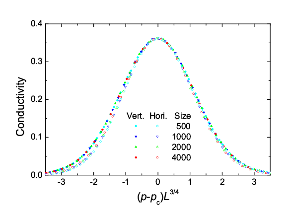
The determination of the critical exponent is based on the fact that near the conductance is a function of a single argument, (vertical scan) or (horizontal scan). Exactly at the conductivity assumes the universal value, found by Cardy [46], which should be the same for the entire boundary.
The scaling analysis was performed for all three models. In Fig. 8 we present results for the model at a particular critical point . Overall, the scaling confirms that both for vertical and horizontal scans. Particular feature about the scaling data is that the widths of scaling functions are slightly different for the vertical and horizontal scans. We have also found that there is a small size effect precisely at the boundary which is well described by the expression
| (30) |
where is a constant.
III.3 Behavior of the localization length at zero field: models and .
We now turn to the behavior of the localization length, , at zero magnetic field, . For each model, the dependence at small is determined by a peculiar behavior of the corresponding delocalization boundary established in subsection A. It is also very important that is equally affected by the second, complementary, boundary in the domain , which is the mirror image of the boundary in Fig. 6.
For moderate , when the boundaries were straight lines [14], the presence of the second boundary leads to the enhancement of . On the contrary, we will see that in the limit , the fact that both boundaries for a given model are almost horizontal leads to a shortening of .

In Fig. 9 we plot the conductivity for model as a function of for and for several values of the system size: 500 (diamonds), 1000 (down triangles), 2000 (up triangles), 4000 (circles) and 8000 (squares). It is seen that the curves for different system sizes have similar shapes and are even-spaced along the logarithmic horizontal axis. Thus we expect scaling and behavior as a consequence. A practical procedure to infer from the data in Fig. 9 is based on the dependence, versus , where is the position of the maximum of the conductivity for a given . In the inset of Fig. 9 we plot in a double logarithmic scale. We see that follows the dependence
| (31) |
where and are model-dependent constants. For model , we found and . Eq. (31) and the fact that is very close to suggest that, to achieve scaling, the data in Fig. 9 should be replotted versus . The result of this replotting is shown in Fig. 10. It is seen that the overlap is excellent, yielding the critical exponent . This should be contrasted to the behavior at any non-zero . We conclude that at the divergence of the localization length with is much slower.

Finally, for the model the plots as a function of do not exhibit maxima. As shown in Fig. 11, where we plot versus , a very good overlap is achieved for .

In conclusion of this subsection we note that the conductivity for all three models tends to as . The reason is that the value at the threshold is the property of a single critical point [46]. By contrast, in our case two critical lines merge at the point, , .
III.4 Behavior of the localization length at zero field: model .
Scaling analysis of the data for model reveals slightly different behaviors for the domains of ”moderate” and ”truly critical” . For the first domain, from the position of peaks we find . This suggests that . Note however that replotting the conductivity versus , see Fig. 12, does not lead to overlap as good as for the model . Moreover, in the second domain a good overlap is achieved for the exponent , i.e., the same as in the model . This is illustrated in the inset of Fig. 12. This indicates that for the model the true critical region is quite narrow. Such a delicate behavior of for the model might indicate that the critical boundary in this model also changes the behavior in the truly critical region .

IV Discussion
IV.1 Position of boundaries
It is seen from Fig. 6 that the boundaries, and , almost coincide in the entire domain, . Overall, these boundaries are in agreement with the results of quantum simulation Ref. 14 shown with black dots. It is also seen that the boundary, , goes significantly higher. In particular, at , exceeds almost twice. On the physical level, this means that, for a given average magnetic field, the formation of edge states requires a longer zero-field mean free path, , for model than for model . In other words, formation of edge states happens easier when a random magnetic field is present. To gain a physical insight why this is so, consider electron motion in random magnetic field. Local value of the field changes its sign in space, while the average field, , is much smaller than the absolute value of the local field. Then electron trajectories are either circles inside the regions where the field maintains its sign, or snake states, propagating along the boundaries of these regions, i.e., along the contours with zero local field. Then it is apparent that a weak disorder does not affect this picture. If, on the other hand, the magnetic field, , is uniform, electron trajectories are big circles. Then a weak disorder will have a strong effect by deflecting electron before it completes a circle. The above two situations correspond to the models and , respectively, and explain why . In model , random component of magnetic field is present, but is weaker than in model . In this regard, the fact that the boundary lies between and , also finds its explanation.
Although quantum simulations are impossible in the domain five ”quantum” data points in Fig. 6 follow within the accuracy of quantum simulations. Then the confirmation of the scaling theory Eqs. (1), (2) would be the linearity of the percolation boundary at , see Eq. (18).
The most important outcome of the present simulation is the inset in Fig. 6. It is seen that at really small and close to the behaviors of all three boundaries changes dramatically compared to their ”bodies”, namely, they become almost horizontal. All three boundaries have the form with . This is in stark contrast to the prediction of scaling theory Eq. (18), which corresponds to . In other words, percolation results suggest that instead of the condition , the delocalization boundary is described by
| (32) |
The latter condition can be also cast in the form Eq. (8) with . We note that the crossover from to Eq. (32) takes place at large . In terms of the flow diagram of the quantum Hall effect [3] this means that the upper part of the vertical flow line is bent to the right, as it is illustrated in Fig. 1b.
IV.2 Semi-analytical consideration
To specify the distinct behavior of percolation boundaries in vanishing average magnetic field they are plotted in Fig. 7 in the log-log scale. From the slopes we deduce the values, , , and . To get a feeling why all -values are close to , below we present some semi-analytical arguments. We first turn to Fig. 5 and set . Then the lattice breaks into two quadratic sublattices with even and odd, which are completely disconnected. None of them percolates if , the percentage of bonds present in each sublattice, is less than . Finite allows percolation for since p-bonds couple clusters from different sublattices. It is apparent that coupling of clusters by p-bonds is relevant if the typical distance, , between two p-bonds become smaller than the localization length, . This yield a constrain that . This constrain is insensitive to the mutual correlations of q-bonds on the two sublattices. In fact, this correlation is absent in model . Indeed, as follows from Eq. (26), at for model we have . By contrast, for model the probabilities at are , . This suggests that q-bonds on two sublattices are strongly (and positively) correlated. Namely, if there is a q-bond connecting two even plaquettes at a given node, then there must be a q-bond connecting odd plaquettes at the same node. On the other hand, the correlation of q-bonds at a node in model is negative: presence of one q-bond excludes the presence of the other. This is apparent from Fig. 4.

As p-bonds are switched on, clusters include sites from both sublattices, see Fig. 13. In Ref. 14 where the model was considered, it was argued that . The argument was based on the following picture of the cluster growth upon increasing : it was assumed that critical q-clusters on a given sublattice grow by getting connected via additional q-bonds. Since the growth of clusters due to p-bonds takes place by connecting critical clusters from different sublattices, it was concluded that p- and q-bonds play equal roles in the growth of clusters, which immediately leads to . Present simulations suggest that in the close proximity of this picture fails, and the role of p- and q-bonds in approaching the percolation threshold is completely different, namely, the growth due to p-bonds is more efficient. This growth proceeds by p-bonds connecting the hulls of critical clusters from two sublattices, as illustrated in Fig. 13. For a given , the length of the hull is
| (33) |
For the model , to achieve a percolation by adding p-bonds one should take into account that the hulls on two sublattices are uncorrelated. Then, a p-bond with one end on a hull from even sublattice will have the other end on the hull from odd sublattice with probability . As a result, the percolation condition reads
| (34) |
where the second factor is the probability that there is at least one p-bond with one end on the critical hull from, say, odd sublattice. Eq. (34) yields , which coincides with the simulation result.
Correlation of q-bonds at the nodes for models and leads to conclusion that corresponding critical clusters in two sublattices are also correlated. One consequence of this correlation is that it takes less p-bonds than in model to connect critical hulls from two sublattices. As a result, , . On the other hand, the picture of percolation by connecting the critical clusters imposes the upper boundary for both models and . This follows from the condition that there should be at least one p-bond per critical hull, i.e., . Note that the constraint is stricter than the constraint , established above.
Beyond the estimate, , we cannot come up with more accurate analytical values for these indices. We are not even able to establish which of them is bigger. This is because strong correlation between the hulls in both models and simplifies connectivity upon switching on p-bonds. On the other hand, this correlation prevents the expansion of the resulting cluster.
As it was established in the previous section, in the domain of , behavior of at in the model exhibits crossover from the critical exponent, , to . To relate this peculiar behavior with the shape of the percolation boundary , we invoke the argument of Ref. 47 which, in application to the p-q model, goes as follows. If the divergence of at the point, , , is characterized by along the q- direction and along the p- direction, then the shape of the critical boundary is , i.e., . Following this argument, crossover in the model from to suggests that and merge in truly critical region.
Overall, our numerical results suggest that in the truly critical domain, where and , the divergence of for all three models is well described by the relation
| (35) |
With regard to the argument of Ref. 47 this means that, for all three models, the exponent is equal to , i.e., the same as for away from .
IV.3 Relation to Ref. 45
In Ref. 45, spin quantum Hall effect in bilayer and trilayer systems was studied numerically, in order to trace the emergence of macroscopic metallic phase upon adding the third dimension [48]. The authors made use of the fact that in a strictly 2D system there is a mapping between the spin quantum Hall transition and classical bond percolation [49, 50]. For bilayer systems the corresponding classical percolation is bond percolation on each layer (bonds connect the centers of plaquettes), complemented with the possibility to switch layers with a probability, , while passing each side of each plaquette. Physically, in spin quantum Hall effect, an electron travels on each layer of the network in the same direction. In our consideration of the weak-field quantum Hall effect, an electron stays within a plane but each link of the square lattice represents two counterpropagating channels. For this reason there is a mapping between the simulation in Ref. 45 and treatment of the model in the present paper. Namely, in Ref. 45 should be identified with the backscattering probability in the present paper, while the probability that the given bond is present in Ref. 45, , should be identified with our parameter . Due to this mapping, critical behavior, for small in Ref. 45, is the same as the behavior of critical line, , for small in our model . Also, the above semi-analytical calculation of is the same as proposed in Ref. 45. However, it should be noted that mapping between the network of Ref. 45 and model applies only for small . For larger the position of the boundary in Ref. 45 differs dramatically from that of the model .
IV.4 Phases with higher
In fact, scaling theory predicts that all Landau levels, , in Eq. (4), eventually levitate to , as the magnetic field is lowered. Our simulations do not capture low-field transitions for . This is because we restricted our consideration to network with one channel per link. Within this description we were able to capture the Drude conductivity tensor of electron gas in a weak field, and weak localization effects. On the other hand, this description does not allow, in principle, to capture the phases with quantized higher than .
As a final remark, we can underscore the difference of the scaling theory and our results as follows. The scaling theory predicts that electron gas experiences a delocalization transition in a magnetic field at which flux into the area is of the order of the flux quantum, . We find that, in the limit of , the interplay of orbital and phase actions of magnetic field causes the transition when this flux is much larger than .
V Acknowledgements
We acknowledge the hospitality of KITP Santa Barbara where this project was initiated. V. V. M. and M. E. R. acknowledge the support of the Grants DOE No. DE-FG02-06ER46313 and BSF No. 2006201, and useful discussions with I. Gruzberg and V. Kagalovsky. M. O. and A. M. S. thank financial support from Spanish DGI Grant No. FIS2009-13483, and from Fundacion Seneca, Grant No. 08832/PI/08.
References
- [1] E. Abrahams, P. W. Anderson, D. C. Licciardello, and T. V. Ramakrishnan, Phys. Rev. Lett. 42, 673 (1979).
- [2] A. M. M. Pruisken, Nucl. Phys. B235, [FS11], 277 (1984); A. M. M. Pruisken and I. S. Burmistrov, Ann. Phys. 316, 285 (2005).
- [3] D. E. Khmelnitskii, Phys. Lett. 106A, 182 (1984); his prediction of levitation was based on analysis of RG flows, which he introduced earlier in JETP Lett. 38, 552 (1983).
- [4] R. Laughlin, Phys. Rev. Lett. 52, 2304 (1984).
- [5] H. W. Jiang, C. E. Johnson, and K. L. Wang, Phys. Rev. B 46, 12830 (1992).
- [6] C. E. Johnson and H. W. Jiang, Phys. Rev. B 48, 2823 (1993).
- [7] H. W. Jiang, C. E. Johnson, K. L. Wang, and S. T. Hannahs, Phys. Rev. Lett. 71, 1439 (1993).
- [8] I. Glozman, C. E. Johnson, and H. W. Jiang, Phys. Rev. Lett. 74, 594 (1995).
- [9] I. Glozman, C. E. Johnson, and H. W. Jiang, Phys. Rev. B 52, R14348 (1995).
- [10] T. Wang, K. P. Clark, G. F. Spencer, A. M. Mack, and W. P. Kirk, Phys. Rev. Lett. 72, 709 (1994).
- [11] J. F. Hughes, J. T. Nicholls, J. E. F. Frost, E. H. Linfield, M. Pepper, C. J. B. Ford, D. A. Ritchie, G. A. C. Jones, E. Kogan, and M. Kaveh, J. Phys.: Condens. Matter 6, 4763 (1994).
- [12] S.-H. Song, D. Shahar, D. C. Tsui, Y. H. Xie, and D. Monroe, Phys. Rev. Lett. 78, 2200 (1997).
- [13] D. J. Thouless, M. Kohmoto, M. P. Nightingale, and M. den Nijs, Phys. Rev. Lett. 49, 405 (1982).
- [14] V. V. Mkhitaryan, V. Kagalovsky, and M. E. Raikh, Phys. Rev. Lett. 103, 066801 (2009); Phys. Rev. B 81, 165426 (2010).
- [15] J. K. Jain, Phys. Rev. Lett. 63, 199 (1989); Phys. Rev. B 40, 8079 (1989); 41, 7653 (1990).
- [16] B. I. Halperin, P. A. Lee, and N. Read, Phys. Rev. B 47, 7312 (1993).
- [17] A. K. Geim, S. V. Dubonos, and A. V. Khaetskii, JETP Lett. 51, 121 (1990).
- [18] S. J. Bending, K. von Klitzing, and K. Ploog, Phys. Rev. Lett. 65, 1060 (1990).
- [19] A. K. Geim, S. J. Bending, and I. V. Grigorieva, Phys. Rev. Lett. 69, 2252 (1992).
- [20] A. Geim, S. J. Bending, I. V. Grigorieva, and M. G. Blamire, Phys. Rev. B 49, 5749 (1994).
- [21] A. Smith, R. Taboryski, L. T. Hansen, C. B. Sørensen, Per Hedegård, and P. E. Lindelof, Phys. Rev. B 50, 14726 (1994).
- [22] F. B. Mancoff, R. M. Clarke, C. M. Marcus, S. C. Zhang, K. Campman, and A. C. Gossard, Phys. Rev. B 51, 13269 (1995).
- [23] G. M. Gusev, U. Gennser, X. Kleber, D. K. Maude, J. C. Portal, D. I. Lubyshev, P. Basmaji, M. de Silva, J. C. Rossi, and Yu. V. Nastaushev, Phys. Rev. B 53, 13641 (1996).
- [24] A. A. Bykov, G. M. Gusev, J. R. Leite, A. K. Bakarov, N. T. Moshegov, M. Cassé, D. K. Maude, and J. C. Portal, Phys. Rev. B 61, 5505 (2000).
- [25] A. W. Rushforth, B. L. Gallagher, P. C. Main, A. C. Neumann, M. Henini, C. H. Marrows, and B. J. Hickey, Phys. Rev. B 70, 193313 (2004).
- [26] A. G. Aronov, A. D. Mirlin, and P. Wölfle, Phys. Rev. B 49, 16609 (1994).
- [27] D. K. K. Lee and J. T. Chalker, Phys. Rev. Lett. 72, 1510 (1994).
- [28] D. K. K. Lee, J. T. Chalker, and D. Y. K. Ko, Phys. Rev. B 50, 5272 (1994).
- [29] D. B. Chklovskii and P. A. Lee, Phys. Rev. B 48, 18060 (1993).
- [30] D. B. Chklovskii, Phys. Rev. B 51, 9895 (1995).
- [31] V. I. Fal’ko, Phys. Rev. B 50, 17406 (1994).
- [32] D. V. Khveshchenko, Phys. Rev. Lett. 77, 1817 (1996).
- [33] A. D. Mirlin, D. G. Polyakov, and P. Wölfle, Phys. Rev. Lett. 80, 2429 (1998).
- [34] A. D. Mirlin, J. Wilke, F. Evers, D. G. Polyakov, and P. Wölfle, Phys. Rev. Lett. 83, 2801 (1999).
- [35] A. D. Mirlin, D. G. Polyakov, F. Evers, and P. Wölfle, Phys. Rev. Lett. 87, 126805 (2001).
- [36] A. V. Izyumov and B. D. Simons, J. Phys. A 32, 5563 (1999).
- [37] A. Shelankov, Phys. Rev. B 62, 3196 (2000).
- [38] H. Mathur and H. U. Baranger, Phys. Rev. B 64, 235325 (2001).
- [39] K. B. Efetov and V. R. Kogan, Phys. Rev. B 70, 195326 (2004).
- [40] D. G. Ravenhall, H. W. Wyld, and R. L. Schult, Phys. Rev. Lett. 62, 1780 (1989).
- [41] H. U. Baranger and A. D. Stone, Phys. Rev. Lett. 63, 414 (1989).
- [42] C. W. Beenakker and H. van Houten, Phys. Rev. Lett. 63, 1857 (1989).
- [43] J. T. Chalker and P. D. Coddington, J. Phys. C 21, 2665 (1988).
- [44] D.-H. Lee, Z. Wang, and S. Kivelson, Phys. Rev. Lett. 70, 4130 (1993).
- [45] J. T. Chalker, M. Ortuño, and A. M. Somoza, Phys. Rev. B 83, 115317 (2011).
- [46] J. L. Cardy, J. Phys. A 35, L565 (2002).
- [47] V. Kagalovsky, B. Horovitz, Y. Avishai, and J. T. Chalker, Phys. Rev. Lett. 82, 3516 (1999).
- [48] M. Ortuño, A. M. Somoza, and J. T. Chalker, Phys. Rev. Lett. 102, 070603 (2009).
- [49] I. A. Gruzberg, A. W. W. Ludwig, and N. Read, Phys. Rev. Lett. 82, 4524 (1999).
- [50] E. J. Beamond, J. Cardy, and J. T. Chalker, Phys. Rev. B 65, 214301 (2002).