跳到论文正文
W Papers独立论文阅读器 arXiv:1105.1229 论文正文 计算阅读时间 · 0%
引用这篇论文根据当前论文元数据生成,正式投稿前建议核对。


License: arXiv.org perpetual non-exclusive license
arXiv:1105.1229v3 [math.AG] 20 Oct 2011

General Tensor Decomposition, Moment Matrices and Applications

A. Bernardi∗ & J. Brachat∗ & P. Comon+ & B. Mourrain∗ Address: ∗ Alessandra Bernardi & Jérôme Brachat & Bernard Mourrain: GALAAD, INRIA Méditerranée
Sophia-Antipolis, France
Email address: [FirstName.LastName]@inria.fr Address: + Pierre Comon:
Laboratoire I3S, CNRS and Univ. of Nice,
Sophia-Antipolis, France
Email address: pcomon@i3s.unice.fr
Abstract.

The tensor decomposition addressed in this paper may be seen as a generalisation of Singular Value Decomposition of matrices. We consider general multilinear and multihomogeneous tensors. We show how to reduce the problem to a truncated moment matrix problem and give a new criterion for flat extension of Quasi-Hankel matrices. We connect this criterion to the commutation characterisation of border bases. A new algorithm is described. It applies for general multihomogeneous tensors, extending the approach of J.J. Sylvester to binary forms. An example illustrates the algebraic operations involved in this approach and how the decomposition can be recovered from eigenvector computation.

Keywords: tensor; decomposition; multihomogeneous polynomial; rank; Hankel operator; moment matrix; flat extension.

1. Introduction

Tensors are objects that appear in various contexts and applications. Matrices are tensors of order two, and are better known than tensors. But in many problems, higher order tensors are naturally used to collect information which depend on more than two variables. Typically, these data could be observations of some experimentation or of a physical phenomenon that depends on several parameters. These observations are stored in a structure called tensor, whose dimensional parameters (or modes) depend on the problem.

The tensor decomposition problem consists of decomposing a tensor (e.g. the set of observations) into a minimal sum of so-called decomposable tensors (i.e. tensors of rank 11). Such a decomposition which is independent of the coordinate system allows to extract geometric or invariant properties associated with the observations. For this reason, the tensor decomposition problem has a large impact in many applications. The first well known case is encountered for matrices (i.e. tensors of order 2), and is related to Singular Value Decomposition with applications e.g. to Principal Component Analysis. Its extension to higher order tensors appears in Electrical Engineering [56], in Signal processing [25], [19], in Antenna Array Processing [29] [16] or Telecommunications [58], [15], [53], [32], [28], in Chemometrics [10] or Psychometrics [38], in Data Analysis [21], [13], [30], [37], [54], but also in more theoretical domains such as Arithmetic complexity [39] [8] [55] [40]. Further numerous applications of tensor decompositions may be found in [19] [22] [54].

From a mathematical point of view, the tensors that we will consider are elements of 𝒯:=Sδ1(E1)⊗⋯⊗Sδk(Ek)\mathcal{T}:=S^{\delta_{1}}(E_{1})\otimes\cdots\otimes S^{\delta_{k}}(E_{k}) where δi∈ℕ\delta_{i}\in\mathbb{N}, EiE_{i} are vector spaces of dimension ni+1n_{i}+1 over a field 𝕂\mathbb{K} (which is of characteristic 00 and algebraically closed), and Sδi​(Ei)S^{\delta_{i}}(E_{i}) is the δith\delta_{i}^{\mathrm{th}} symmetric power of EiE_{i}. The set of tensors of rank 11 form a projective variety which is called the Veronese variety when k=1k=1 or the Segre variety when δi=1,i=1,…,k\delta_{i}=1,i=1,\ldots,k. We will call it hereafter the Segre-Veronese variety of ℙ⁡(𝒯)\mathbb{P}(\mathcal{T}) and denote it Ξ⁡(𝒯)\Xi(\mathcal{T}). The set of tensors which are the linear combinations of rr elements of the Segre-Veronese variety are those which admit a decomposition with at most rr terms of rank 11 (i.e. in Ξ⁡(𝒯)\Xi(\mathcal{T})). The closure of this set is called the rr-secant variety and denoted Ξr​(𝒯)\Xi_{r}(\mathcal{T}). More precise definitions of these varieties will be given in Sec. 2.3.

Decomposing a tensor TT consists of finding the minimal rr such that this tensor is a sum of rr tensors of rank 11. This minimal rr is called the rank of TT. By definition, a tensor of rank rr is in the secant variety Ξr​(𝒯)\Xi_{r}(\mathcal{T}). Thus analysing the properties of these secant varieties and their characterisation helps determining tensor ranks and decompositions.

The case where k=2k=2 and δ1=δ2=1\delta_{1}=\delta_{2}=1 corresponds to the matrix case, which is well known. The rank of a matrix seen as a tensor of order k=2k=2 is its usual rank. The case where k=1k=1 and δ1=2\delta_{1}=2 corresponds to the case of quadratic forms and is also well understood. The rank of the symmetric tensor is the usual rank of the associated symmetric matrix. The case where k=1k=1, δ1∈ℕ\delta_{1}\in\mathbb{N} and n1=1n_{1}=1 corresponds to binary forms, which has been analyzed by J.J. Sylvester in [57]. A more complete description in terms of secant varieties is given in [44].

On our knowledge if k>1k>1 and if at least one of the δi\delta_{i}’s is larger than 11, then there is no specific result in the literature on the defining ideal of secant varieties of Segre-Veronese varieties Ξ(Sδ1(E1)⊗⋯⊗Sδk(Ek))\Xi(S^{\delta_{1}}(E_{1})\otimes\cdots\otimes S^{\delta_{k}}(E_{k})) except for [14] where the authors conjecture that when OPENΞr​(Sδ1​(E1)⊗Sδ2​(E2)))\Xi_{r}(S^{\delta_{1}}(E_{1})\otimes S^{\delta_{2}}(E_{2}))) is a defective hypersurface, then its defining equation is a determinantal equation.

In the case of the secant varieties of Veronese varieties (i.e. if k=1k=1 and δ1>1\delta_{1}>1), the knowledge of their ideal is sparse. Beside the classical results (see one for all [36]) we quote [43] as the most up-to-date paper on that subject. We also quote [44] for a modern approach to equations of secant varieties in general using representation theory.

About the case of secant varieties of Segre varieties (i.e. δi=1\delta_{i}=1 for i=1,…,ki=1,\ldots,k) the only obvious case is the 22 factors Segre. For some of the non trivial cases in which equations of secant varieties of Segre varieties are known we refer to [41], [45], [2], [14].

The first method to compute such a decomposition, besides the case of matrices or quadratic forms which may go back to the Babylonians, is due to Sylvester for binary forms [57]. Using apolarity, kernels of catalecticant matrices are computed degree by degree until a polynomial with simple roots is found. See also [20], [36]. An extension of this approach for symmetric tensors has been analyzed in [36], and yields a decomposition method in some cases (see [36][p. 187]). Some decomposition methods are also available for specific degrees and dimensions, e.g. using invariant theory [24]. In [7], there is a simplified version of Sylvester’s algorithm, which uses the mathematical interpretation of the problem in terms of secant varieties of rational normal curves. The same approach is used in [7] to give algorithms for the decompositions of symmetric tensors belonging to Ξ2​(Sd​(E))\Xi_{2}(S^{d}(E)) and to Ξ3​(Sd​(E))\Xi_{3}(S^{d}(E)). In [4] a complete rank stratification of Ξ4​(Sd​(E))\Xi_{4}(S^{d}(E)) is given.

In [9], Sylvester’s approach is revisited from an affine point of view and a general decomposition method based on a flat extension criterion is described. The main contribution of the current paper is to extend this method to more general tensor spaces including classical multilinear tensors and multihomogeneous tensors. In particular we give a new and more flexible criterion for the existence of a decomposition of a given rank, which extends non trivially the result in [47] and the characterization used in [9]. This criterion is a rank condition of an associated Hankel operator. Moreover we use that criterion to write a new algorithm which checks, degree by degree, if the roots deduced from the kernel of the Hankel operator are simple. This allows to compute the rank of any given partially symmetric tensor.

This paper is an extended version of [6], with the complete proofs and with detailed examples.

In Sec. 2, we recall the notations, the geometric point related to secants of Segre and Veronese varieties, and the algebraic point of view based on moment matrices. In Sec. 3, we describe the algorithm and the criterion used to solve the truncated moment problem. In Sec. 4, an example of tensor decompositions from Antenna Array Processing illustrates the approach.

2. Duality, moment matrices and tensor decomposition

2.1. Notation and preliminaries

Let 𝕂\mathbb{K} be an algebraically closed field (e.g. 𝕂=ℂ\mathbb{K}=\mathbb{C} the field of complex numbers). We assume that 𝕂\mathbb{K} is of characteristic 00. For a vector space EE, its associated projective space is denoted ℙ⁡(E)\mathbb{P}(E). For \bvec​v∈E−{0}\bvec{v}\in E-\{0\} its class in ℙ⁡(E)\mathbb{P}(E) is denoted \bvec​v¯\overline{\bvec{v}}. Let ℙn\mathbb{P}^{n} be the projective space of E:=𝕂n+1E:=\mathbb{K}^{n+1}. For a subset F={f1,…,fm}F=\{f_{1},\dots,f_{m}\} of a vector-space (resp. ring) RR, we denote by ⟨F⟩\langle F\rangle (resp. (F)(F)) the vector space (resp. ideal) generated by FF in RR.

We consider hereafter the symmetric δ\delta-th power Sδ​(E)S^{\delta}(E) where EE is a vector space of basis x0,…,xnx_{0},\ldots,x_{n}. An element of Sδ​(E)S^{\delta}(E) is a homogeneous polynomial of degree δ∈ℕ\delta\in\mathbb{N} in the variables 𝐱=(x0,…,xn)\mathbf{x}=(x_{0},\ldots,x_{n}). For 𝐱1=(x0,1,…,xn1,1)\mathbf{x}_{1}=(x_{0,1},\ldots,x_{n_{1},1}) ,…,,\ldots, 𝐱k=(x0,k,…,xnk,k)\mathbf{x}_{k}=(x_{0,k},\ldots,x_{n_{k},k}), Sδ1(E1)⊗⋯⊗Sδk(Ek)S^{\delta_{1}}(E_{1})\otimes\cdots\otimes S^{\delta_{k}}(E_{k}) (with Ei=⟨x0,i,…,xni,i⟩E_{i}=\langle x_{0,i},\ldots,x_{n_{i},i}\rangle) is the vector space of polynomials multihomogeneous of degree δi\delta_{i} in the variables 𝐱i\mathbf{x}_{i}.

Hereafter, we will consider the deshomogeneisation of elements in Sδ1(E1)⊗⋯⊗Sδk(Ek)S^{\delta_{1}}(E_{1})\otimes\cdots\otimes S^{\delta_{k}}(E_{k}), obtained by setting x0,i=1x_{0,i}=1 for i=1,…,ki=1,\ldots,k. We denote by Rδ1,…,δkR_{\delta_{1},\ldots,\delta_{k}} this space, where R=𝕂⁡[𝐱¯1,…,𝐱¯k]R=\mathbb{K}[\underline{\mathbf{x}}_{1},\ldots,\underline{\mathbf{x}}_{k}] is the space of polynomials in the variables 𝐱¯1=(x1,1,…,xn1,1),…,𝐱¯k=(x1,k,…,xnk,k)\underline{\mathbf{x}}_{1}=(x_{1,1},\ldots,x_{n_{1},1}),\ldots,\underline{\mathbf{x}}_{k}=(x_{1,k},\ldots,x_{n_{k},k}).

For αi=(α1,i,…,αni,i)∈ℕni\alpha_{i}=(\alpha_{1,i},\ldots,\alpha_{n_{i},i})\in\mathbb{N}^{n_{i}} (i=1,…,ki=1,\ldots,k), let 𝐱¯iαi=∏j=1nixj,iαj,i\underline{\mathbf{x}}_{i}^{\alpha_{i}}=\prod_{j=1}^{n_{i}}x_{j,i}^{\alpha_{j,i}}, |\bvec​αi|=∑j=1niαj,i|\bvec{\alpha_{i}}|=\sum_{j=1}^{n_{i}}{\alpha_{j,i}}, and 𝐱¯α=∏j=1ni𝐱iαi\underline{\mathbf{x}}^{\alpha}=\prod_{j=1}^{n_{i}}\mathbf{x}_{i}^{\alpha_{i}}.

An element ff of Rδ=Rδ1,…,δkR_{\delta}=R_{\delta_{1},\ldots,\delta_{k}} is represented as

f=∑\bvec​α=(\bvec​α1,…,\bvec​αk);|\bvec​αi|≤δif\bvec​α𝐱¯1α1⋯𝐱¯kαk.f=\sum_{\bvec{\alpha}=(\bvec{\alpha}_{1},\ldots,\bvec{\alpha}_{k});|\bvec{\alpha}_{i}|\leq\delta_{i}}f_{\bvec{\alpha}}\,\underline{\mathbf{x}}_{1}^{\alpha_{1}}\cdots\underline{\mathbf{x}}_{k}^{\alpha_{k}}.

The dimension of Rδ:=Rδ1,…,δkR_{\delta}:=R_{\delta_{1},\ldots,\delta_{k}} is nδ1,…,δk;n1,…,nkn_{\delta_{1},\ldots,\delta_{k};n_{1},\ldots,n_{k}} == ∏i=1k(ni+δiδi)\prod_{i=1}^{k}{n_{i}+\delta_{i}\choose\delta_{i}}. For δ∈ℕ,α∈ℕn\delta\in\mathbb{N},\alpha\in\mathbb{N}^{n} with |α|≤δ|\alpha|\leq\delta, let (δα)=δ!α1!⋯αn!(δ−|α|)!{\delta\choose\alpha}={\delta!\over\alpha_{1}!\cdots\alpha_{n}!(\delta-|\alpha|)!}. We define the apolar inner product on Rδ1,…,δkR_{\delta_{1},\ldots,\delta_{k}} by ⟨f|g⟩=∑|αi|≤δifαgα(δ1α1)⋯(δkαk).\langle f|g\rangle=\sum_{|\alpha_{i}|\leq\delta_{i}}f_{\alpha}\,g_{\alpha}{\delta_{1}\choose\alpha_{1}}\cdots{\delta_{k}\choose\alpha_{k}}.

The dual space of a 𝕂\mathbb{K}-vector space EE is denoted E∗=Hom𝕂⁡(E,𝕂){E}^{*}=\operatorname{Hom}_{\mathbb{K}}(E,\mathbb{K}). It is the set of 𝕂\mathbb{K}-linear forms from EE to 𝕂\mathbb{K}. A basis of the dual space Rδ∗{R}^{*}_{\delta}, is given by the set of linear forms that compute the coefficients of a polynomial in the monomial basis (𝐱¯α)α∈ℕn1×⋯×ℕnk;|αi|≤δi(\underline{\mathbf{x}}^{{\alpha}})_{\alpha\in\mathbb{N}^{n_{1}}\times\cdots\times\mathbb{N}^{n_{k}};|\alpha_{i}|\leq\delta_{i}}. We denote it by (𝐝α)α∈ℕn1×⋯×ℕnk;|αi|≤δi(\mathbf{d}^{{\alpha}})_{\alpha\in\mathbb{N}^{n_{1}}\times\cdots\times\mathbb{N}^{n_{k}};|\alpha_{i}|\leq\delta_{i}}. We identify R∗{R}^{*} with the (vector) space of formal power series 𝕂⁡[[𝐝]]\mathbb{K}[[\mathbf{d}]] = 𝕂[[𝐝1,…,𝐝k]]=𝕂[[d1,1,…,dn1,1\mathbb{K}[[\mathbf{d}_{1},\ldots,\mathbf{d}_{k}]]=\mathbb{K}[[d_{1,1},\dots,d_{n_{1},1}, …\ldots, d1,k,…,dnk,k]]d_{1,k},\dots,d_{n_{k},k}]]. Any element Λ∈R∗\Lambda\in{R}^{*} can be decomposed as

Λ=∑α∈ℕn1×⋯×ℕnkΛ(𝐱α)𝐝α.\Lambda=\sum_{\alpha\in\mathbb{N}^{n_{1}}\times\cdots\times\mathbb{N}^{n_{k}}}\,\Lambda(\mathbf{x}^{\alpha})\,\mathbf{d}^{\alpha}.

Typical elements of R∗{R}^{*} are the linear forms that correspond to the evaluation at a point ζ=(ζ1,…,ζi)∈𝕂n1×⋯×𝕂nk\zeta=(\zeta_{1},\ldots,\zeta_{i})\in\mathbb{K}^{n_{1}}\times\cdots\times\mathbb{K}^{n_{k}}:

𝟏ζ:R→𝕂p↦p⁡(ζ)\begin{array}[]{lcl}\mathbf{1}_{\zeta}&:&R\rightarrow\mathbb{K}\\ &&p\mapsto p(\zeta)\\ \end{array}

The decomposition of 𝟏ζ\mathbf{1}_{\zeta} in the basis {\bvecd\bvec​α}\bvecα∈ℕn1×⋯×ℕnk\{\bvec{d}^{\bvec{\alpha}}\}_{\bvec{\alpha}\in\mathbb{N}^{n_{1}}\times\cdots\times\mathbb{N}^{n_{k}}} is

𝟏ζ=∑α∈ℕn1×⋯×ℕnkζα𝐝α=∑α∈ℕn1×⋯×ℕnk∏i=1kζiαi𝐝iαi.\mathbf{1}_{\zeta}=\sum_{\alpha\in\mathbb{N}^{n_{1}}\times\cdots\times\mathbb{N}^{n_{k}}}\zeta^{\alpha}\,\mathbf{d}^{\alpha}=\sum_{\alpha\in\mathbb{N}^{n_{1}}\times\cdots\times\mathbb{N}^{n_{k}}}\prod_{i=1}^{k}\zeta_{i}^{\alpha_{i}}\,\mathbf{d}_{i}^{\alpha_{i}}.

We recall that the dual space R∗{R}^{*} has a natural structure of RR-module [31] which is defined as follows: for all p∈Rp\in R, and for all Λ∈R∗\Lambda\in{R}^{*} consider the linear operator

p⋆Λ:R→𝕂q↦Λ⁡(p​q).\begin{array}[]{lcl}p\star\Lambda&:&R\rightarrow\mathbb{K}\\ &&q\mapsto\Lambda(pq).\end{array}

In particular, we have xi,j⋆𝐝1α1⋯𝐝jαj⋯𝐝kαk=x_{i,j}\star\mathbf{d}_{1}^{\alpha_{1}}\cdots\mathbf{d}_{j}^{\alpha_{j}}\cdots\mathbf{d}_{k}^{\alpha_{k}}=
𝐝1α1⋯𝐝j−1αj−1d1,jα1,j⋯di−1,jαi−1,jdi,jαi,j−1di+1,jαi+1,j⋯dnj,jαnj,j𝐝j+1αj+1⋯𝐝kαk\mathbf{d}_{1}^{\alpha_{1}}\cdots\mathbf{d}_{j-1}^{\alpha_{j-1}}\,d_{1,j}^{\alpha_{1,j}}\cdots d_{i-1,j}^{\alpha_{i-1,j}}d_{i,j}^{\alpha_{i,j}-1}d_{i+1,j}^{\alpha_{i+1,j}}\cdots d_{n_{j},j}^{\alpha_{n_{j},j}}\,\mathbf{d}_{j+1}^{\alpha_{j+1}}\cdots\mathbf{d}_{k}^{\alpha_{k}} if αi,j>0\alpha_{i,j}>0 and 00 otherwise.

2.2. Tensor decomposition

In this section, we present different formulations of the tensor decomposition problem, that we consider in this paper.

We will consider hereafter a partially symmetric tensor TT of Sδ1(E1)⊗⋯⊗Sδk(Ek)S^{\delta_{1}}(E_{1})\otimes\cdots\otimes S^{\delta_{k}}(E_{k}) where Ei=⟨x0,i,…,xni,i⟩E_{i}=\langle x_{0,i},\ldots,x_{n_{i},i}\rangle. It can be represented by a partially symmetric array of coefficients

(1) [T]=(Tα1,…,αk)αi∈ℕni+1;|αi|=δi.[T]=(T_{\alpha_{1},\ldots,\alpha_{k}})_{\alpha_{i}\in\mathbb{N}^{n_{i}+1};|{\alpha}_{i}|=\delta_{i}}.

For αi∈ℕni\alpha_{i}\in\mathbb{N}^{n_{i}} with |αi|≤δi|\alpha_{i}|\leq\delta_{i}, we denote α¯i=(δi−|αi|,α1,i,…CLOSE\overline{\alpha}_{i}=(\delta_{i}-|\alpha_{i}|,\alpha_{1,i},\ldots, OPENαni,i)\alpha_{n_{i},i}) and, with an abuse of notation, we identify Tα1,…,αk:=Tα1¯,…,αk¯T_{\alpha_{1},\ldots,\alpha_{k}}:=T_{\overline{\alpha_{1}},\ldots,\overline{\alpha_{k}}}.

Such a tensor is naturally associated with a (multihomogeneous) polynomial in the variables 𝐱1=(x0,1,…,xn1,1)\mathbf{x}_{1}=(x_{0,1},\ldots,x_{n_{1},1}), …\ldots, 𝐱k=(x0,k,…,xnk,k)\mathbf{x}_{k}=(x_{0,k},\ldots,x_{n_{k},k})

T(𝐱)=∑α=(α1,…,αk)∈ℕn1×⋯×ℕnk;|αi|≤δiTα𝐱1α¯1⋯𝐱kα¯k.T(\mathbf{x})=\sum_{{{\alpha}=({\alpha}_{1},\ldots,{\alpha}_{k})\in\mathbb{N}^{n_{1}}\times\cdots\times\mathbb{N}^{n_{k}};}\atop{|{\alpha}_{i}|\leq\delta_{i}}}T_{{\alpha}}\,\mathbf{x}_{1}^{{\overline{\alpha}_{1}}}\cdots\mathbf{x}_{k}^{\overline{\alpha}_{k}}.

or to an element T¯​(𝐱¯)∈Rδ1,…,δk\underline{T}(\underline{\mathbf{x}})\in R_{\delta_{1},\ldots,\delta_{k}} obtained by substituting x0,ix_{0,i} by 11 in T⁡(𝐱)T(\mathbf{x}) (for i=1,…,ki=1,\ldots,k):

T¯(𝐱¯)=∑α∈ℕn1×⋯×ℕnk;|αi|≤δiTα𝐱¯1α1⋯𝐱¯kαk.\underline{T}(\underline{\mathbf{x}})=\sum_{\alpha\in\mathbb{N}^{n_{1}}\times\cdots\times\mathbb{N}^{n_{k}};\atop|{\alpha}_{i}|\leq\delta_{i}}T_{{\alpha}}\,\underline{\mathbf{x}}_{1}^{\alpha_{1}}\cdots\underline{\mathbf{x}}_{k}^{\alpha_{k}}.

An element of R∗=𝕂⁡[[𝐝]]R^{*}=\mathbb{K}[[\mathbf{d}]] can also be associated naturally with TT:

T∗(𝐝)=∑α∈ℕn1×⋯×ℕnk;|αi|≤δi(δ1α1)−1⋯(δkαk)−1Tα𝐝1α1⋯𝐝kαk.{T^{*}}(\mathbf{d})=\sum_{\alpha\in\mathbb{N}^{n_{1}}\times\cdots\times\mathbb{N}^{n_{k}};\atop|{\alpha}_{i}|\leq\delta_{i}}{\delta_{1}\choose\alpha_{1}}^{-1}\cdots{\delta_{k}\choose\alpha_{k}}^{-1}T_{{\alpha}}\,\mathbf{d}_{1}^{\alpha_{1}}\cdots\mathbf{d}_{k}^{\alpha_{k}}.

so that for all T′∈Rδ1,…,δkT^{\prime}\in R_{\delta_{1},\ldots,\delta_{k}},

⟨T⁡(𝐱¯)|T′​(𝐱¯)⟩=T∗​(𝐝)​(T′​(𝐱¯)).\langle T(\underline{\mathbf{x}})|T^{\prime}(\underline{\mathbf{x}})\rangle=T^{*}(\mathbf{d})(T^{\prime}(\underline{\mathbf{x}})).

The decomposition of tensor TT can be stated as follows:

Tensor decomposition problem. Given T⁡(𝐱)∈Sδ1​(E1)T(\mathbf{x})\in S^{\delta_{1}}(E_{1}) ⊗⋯⊗Sδk​(Ek)\otimes\cdots\otimes S^{\delta_{k}}(E_{k}), find a decomposition of T⁡(𝐱)T(\mathbf{x}) as a sum of products of powers of linear forms in 𝐱j\mathbf{x}_{j}:

(2) T(𝐱)=∑i=1rγi𝐥1,i(𝐱1)δ1⋯𝐥k,i(𝐱k)δkT(\mathbf{x})=\sum_{i=1}^{r}\,\gamma_{i}\,\mathbf{l}_{1,i}(\mathbf{x}_{1})^{\delta_{1}}\cdots\mathbf{l}_{k,i}(\mathbf{x}_{k})^{\delta_{k}}

where γi≠0\gamma_{i}\neq 0, 𝐥j,i​(𝐱j)=l0,j,i​x0,j+l1,j,i​x1,j+⋯+lnj,j,i​xj,nj\mathbf{l}_{j,i}(\mathbf{x}_{j})=l_{0,j,i}x_{0,j}+l_{1,j,i}x_{1,j}+\cdots+l_{n_{j},j,i}x_{j,n_{j}} and rr is the smallest possible integer for such a decomposition.

Definition 2.1.

The minimal number of terms rr in a decomposition of the form (2) is called the rank of TT.

We say that T⁡(𝐱)T(\mathbf{x}) has an affine decomposition if there exists a minimal decomposition of T⁡(𝐱)T(\mathbf{x}) of the form (2) where rr is the rank of TT and such that l0,j,i≠0l_{0,j,i}\neq 0 for i=1,…,ri=1,\ldots,r. Notice that by a generic change of coordinates in EiE_{i}, we may assume that all l0,j,i≠0l_{0,j,i}\neq 0 and thus that TT has an affine decomposition. Suppose that T⁡(𝐱)T(\mathbf{x}) has an affine decomposition. Then by scaling 𝐥j,i​(𝐱j)\mathbf{l}_{j,i}(\mathbf{x}_{j}) and multiplying γi\gamma_{i} by the inverse of the δjt​h\delta_{j}^{th} power of this scaling factor, we may assume that l0,j,i=1l_{0,j,i}=1. Thus, the polynomial

T¯(𝐱¯)=∑i=1rγi∑|αi|≤δi(δ1α1)⋯(δkαk)ζ1,iα1⋯ζk,iαk𝐱¯1α1⋯𝐱¯kαk\underline{T}(\underline{\mathbf{x}})=\sum_{i=1}^{r}\,\gamma_{i}\,\sum_{|\alpha_{i}|\leq\delta_{i}}\,{\delta_{1}\choose\alpha_{1}}\cdots{\delta_{k}\choose\alpha_{k}}\,\zeta_{1,i}^{\alpha_{1}}\cdots\zeta_{k,i}^{\alpha_{k}}\,\underline{\mathbf{x}}_{1}^{\alpha_{1}}\cdots\underline{\mathbf{x}}_{k}^{\alpha_{k}}

with Tα1,…,αk=∑i=1rγi∑|αi|≤δi(δ1α1)⋯(δkαk)ζ1,iα1⋯ζk,iαkT_{\alpha_{1},\ldots,\alpha_{k}}=\sum_{i=1}^{r}\,\gamma_{i}\,\sum_{|\alpha_{i}|\leq\delta_{i}}{\delta_{1}\choose\alpha_{1}}\cdots{\delta_{k}\choose\alpha_{k}}\,\zeta_{1,i}^{\alpha_{1}}\cdots\zeta_{k,i}^{\alpha_{k}}. Equivalently, we have

T∗(𝐝)=∑i=1rγi∑|αi|≤δiζ1,iα1⋯ζk,iαk𝐝1α1⋯𝐝kαkT^{*}(\mathbf{d})=\sum_{i=1}^{r}\,\gamma_{i}\,\sum_{|\alpha_{i}|\leq\delta_{i}}\,\zeta_{1,i}^{\alpha_{1}}\cdots\zeta_{k,i}^{\alpha_{k}}\,\mathbf{d}_{1}^{\alpha_{1}}\cdots\mathbf{d}_{k}^{\alpha_{k}}

so that T∗​(𝐝)T^{*}(\mathbf{d}) coincides on Rδ1,…,δkR_{\delta_{1},\ldots,\delta_{k}} with the linear form

∑i=1rγi​ 1ζ1,i,…,ζk,i=∑i=1rγi​ 1ζi\sum_{i=1}^{r}\,\gamma_{i}\,\mathbf{1}_{\zeta_{1,i},\ldots,\zeta_{k,i}}=\sum_{i=1}^{r}\,\gamma_{i}\,\mathbf{1}_{\zeta_{i}}

with ζi:=(ζ1,i,…,ζk,i)∈𝕂n1×⋯𝕂nk\zeta_{i}:=(\zeta_{1,i},\ldots,\zeta_{k,i})\in\mathbb{K}^{n_{1}}\times\cdots\mathbb{K}^{n_{k}}.

The decomposition problem can then be restated as follows:

Interpolation problem. Given T∗∈Rδ1,…,δk∗T^{*}\in R_{\delta_{1},\ldots,\delta_{k}}^{*} which admits an affine decomposition, find the minimal number of non-zero vectors ζ1,…,ζr∈𝕂n1×⋯×𝕂nk\zeta_{1},\ldots,\zeta_{r}\in\mathbb{K}^{n_{1}}\times\cdots\times\mathbb{K}^{n_{k}} and non-zero scalars γ1,…,γr∈𝕂−{0}\gamma_{1},\ldots,\gamma_{r}\in\mathbb{K}-\{0\} such that

(3) T∗=∑i=1rγi​ 1ζiT^{*}=\sum_{i=1}^{r}\gamma_{i}\,\mathbf{1}_{\zeta_{i}}

on Rδ1,…,δkR_{\delta_{1},\ldots,\delta_{k}}.

If such a decomposition exists, we say that Λ=∑i=1rγi​ 1ζi∈R∗\Lambda=\sum_{i=1}^{r}\gamma_{i}\,\mathbf{1}_{\zeta_{i}}\in R^{*} extends T∗∈Rδ1,…,δk∗T^{*}\in R_{\delta_{1},\ldots,\delta_{k}}^{*}.

2.3. Decomposable tensors

In this section, we analyze the set of tensors of rank 11, also called decomposable tensors [1]. They naturally form projective varieties, which we are going to describe using the language of projective geometry.

We begin by defining two auxiliary but very classical varieties, namely Segre and Veronese varieties.

Definition 2.2.

The image of the following map

sk:ℙ(E1)×⋯×ℙ(Ek)→ℙ(E1⊗⋯⊗Ek)(\bvec​v1¯,…,\bvec​vk¯)↦\bvecv1⊗⋯⊗\bvecvk¯\begin{array}[]{rcl}s_{k}:\mathbb{P}(E_{1})\times\cdots\times\mathbb{P}(E_{k})&\rightarrow&\mathbb{P}(E_{1}\otimes\cdots\otimes E_{k})\\ (\overline{\bvec{v}_{1}},\ldots,\overline{\bvec{v}_{k}})&\mapsto&\overline{\bvec{v}_{1}\otimes\cdots\otimes\bvec{v}_{k}}\end{array}

is the so called Segre variety of kk factors. We denote it by Ξ(E1⊗⋯⊗Ek)\Xi(E_{1}\otimes\cdots\otimes E_{k}).

From Definition 2.1 of the rank of a tensor and from the Interpolation Problem point of view (3) we see that a Segre variety parametrizes projective classes of rank 1 tensors T=\bvecv1⊗⋯⊗\bvecvk∈E1⊗⋯⊗EkT=\bvec{v_{1}}\otimes\cdots\otimes\bvec{v_{k}}\in E_{1}\otimes\cdots\otimes E_{k} for certain \bvec​vi∈Ei\bvec{v_{i}}\in E_{i}, i=1,…,ki=1,\ldots,k.

Definition 2.3.

Let (J1,J2)(J_{1},J_{2}) be a partition of the set {1,…,k}\{1,\ldots,k\}. If J1={h1,…,hs}J_{1}=\{h_{1},\ldots,h_{s}\} and J2={1,…,k}\J1={h1′,…,hk−s′}J_{2}=\{1,\ldots,k\}\backslash J_{1}=\{h^{\prime}_{1},\ldots,h^{\prime}_{k-s}\}, the (J1,J2)(J_{1},J_{2})-Flattening of E1⊗⋯⊗EkE_{1}\otimes\cdots\otimes E_{k} is the following:

EJ1⊗EJ2=(Eh1⊗⋯⊗Ehs)⊗(Eh1′⊗⋯⊗Ehk−s′).E_{J_{1}}\otimes E_{J_{2}}=(E_{h_{1}}\otimes\cdots\otimes E_{h_{s}})\otimes(E_{h^{\prime}_{1}}\otimes\cdots\otimes E_{h^{\prime}_{k-s}}).

Let EJ1⊗EJ2E_{J_{1}}\otimes E_{J_{2}} be any flattening of E1⊗⋯⊗EkE_{1}\otimes\cdots\otimes E_{k} as in Definition 2.3 and let fJ1,J2:ℙ(E1⊗⋯⊗Ek)→ℙ(EJ1⊗EJ2)f_{J_{1},J_{2}}:\mathbb{P}(E_{1}\otimes\cdots\otimes E_{k})\rightarrow\mathbb{P}(E_{J_{1}}\otimes E_{J_{2}}) be the obvious isomorphism. Let [T][T] be an array associated with a tensor T∈E1⊗⋯⊗EkT\in E_{1}\otimes\cdots\otimes E_{k}; let T′¯=fJ1,J2​(\bvec​T¯)∈ℙ⁡(EJ1⊗EJ2)\overline{T^{\prime}}=f_{J_{1},J_{2}}(\overline{\bvec{T}})\in\mathbb{P}(E_{J_{1}}\otimes E_{J_{2}}) and let [AJ1,J2][A_{J_{1},J_{2}}] be the matrix associated with T′T^{\prime}. Then the dd-minors of the matrix [AJ1,J2][A_{J_{1},J_{2}}] are said to be dd-minors of [T][T].

An array [A]=(xi1,…,ik)0≤ij≤nj,j=1,…,k[A]=(x_{i_{1},\ldots,i_{k}})_{0\leq i_{j}\leq n_{j}\,,\,j=1,\ldots,k} is said to be a generic array of indeterminates of R=𝕂[𝐱¯1,…R=\mathbb{K}[\underline{\mathbf{x}}_{1},\ldots, 𝐱¯k]\underline{\mathbf{x}}_{k}] if the entries of [A][A] are the independent variables of RR.

It is a classical result due to R. Grone (see [34]) that a set of equations for a Segre variety is given by all the 22-minors of a generic array. In [35] it is proved that, if [A][A] is a generic array in RR of size (n1+1)×⋯×(nk+1)(n_{1}+1)\times\cdots\times(n_{k}+1) and Id​([A])I_{d}([A]) is the ideal generated by the dd-minors of [A][A] , then I2​([A])I_{2}([A]) is a prime ideal, therefore:

I(Ξ(E1⊗⋯⊗Ek))=I2([A]).I(\Xi(E_{1}\otimes\cdots\otimes E_{k}))=I_{2}([A]).

We introduce now the Veronese variety. Classically it is defined to be the dd-tuple embedding of ℙn\mathbb{P}^{n} into ℙ(n+dd)−1\mathbb{P}^{{n+d\choose d}-1} via the linear system associated with the sheaf 𝒪⁡(d)\mathcal{O}(d) with d>0d>0. We give here an equivalent definition.

Let EE be an n+1n+1 dimensional vector space. With the notation Sd​(E)S^{d}(E) we mean the vector subspace of E⊗dE^{\otimes d} of symmetric tensors.

Definition 2.4.

The image of the following map

νd:ℙ⁡(E)→ℙ​(Sd​(E))\bvec​v¯↦\bvec​v⊗d¯\begin{array}[]{rcl}\nu_{d}:\mathbb{P}(E)&\rightarrow&\mathbb{P}(S^{d}(E))\\ \overline{\bvec{v}}&\mapsto&\overline{\bvec{v^{\otimes d}}}\end{array}

is the so called Veronese variety. We indicate it with Ξ​(Sd​(E))\Xi(S^{d}(E)).

With this definition it is easy to see that the Veronese variety parametrizes symmetric rank 1 tensors.

Observe that if we take the vector space EE to be a vector space of linear forms ⟨x0,…,xn⟩\langle x_{0},\ldots,x_{n}\rangle then the image of the map νd\nu_{d} above parametrizes homogeneous polynomials that can be written as dd-th powers of linear forms.

The Veronese variety Ξ⁡(Sd​(E))⊂ℙ⁡(Sd​(E))\Xi(S^{d}(E))\subset\mathbb{P}(S^{d}(E)) can be also viewed as Ξ⁡(Sd​(E))=Ξ⁡(E⊗d)∩ℙ⁡(Sd​(E))\Xi(S^{d}(E))=\Xi(E^{\otimes d})\cap\mathbb{P}(S^{d}(E)).

Let [A]=(xi1,…,id)0≤ij≤n,j=1,…,d[A]=(x_{i_{1},\ldots,i_{d}})_{0\leq i_{j}\leq n,\,j=1,\ldots,d} be a generic symmetric array. It is a known result that:

(4) I⁡(Ξ⁡(Sd​(E)))=I2​([A]).I(\Xi(S^{d}(E)))=I_{2}([A]).

See [59] for the set theoretical point of view. In [52] the author proved that I​(Ξ​(Sd​(E)))I(\Xi(S^{d}(E))) is generated by the 22-minors of a particular catalecticant matrix (for a definition of “Catalecticant matrices” see e.g. either [52] or [33]). A. Parolin, in his PhD thesis ([51]), proved that the ideal generated by the 22-minors of that catalecticant matrix is actually I2​([A])I_{2}([A]).

We are now ready to describe the geometric object that parametrizes partially symmetric tensors T∈Sδ1(E1)⊗⋯⊗Sδk(Ek)T\in S^{\delta_{1}}(E_{1})\otimes\cdots\otimes S^{\delta_{k}}(E_{k}). Let us start with the rank 1 partially symmetric tensors.

Definition 2.5.

Let E1,…,EkE_{1},\ldots,E_{k} be vector spaces of dimensions n1+1,…,nk+1n_{1}+1,\ldots,n_{k}+1 respectively. The Segre-Veronese variety Ξ(Sδ1(E1)⊗⋯⊗Sδk(Ek))\Xi(S^{\delta_{1}}(E_{1})\otimes\cdots\otimes S^{\delta_{k}}(E_{k})) is the embedding of ℙ(E1)⊗⋯⊗ℙ(Ek)\mathbb{P}(E_{1})\otimes\cdots\otimes\mathbb{P}(E_{k}) into ℙN−1≃ℙ(Sδ1(E1)⊗⋯⊗Sδk(Ek))\mathbb{P}^{N-1}\simeq\mathbb{P}(S^{\delta_{1}}(E_{1})\otimes\cdots\otimes S^{\delta_{k}}(E_{k})), where N=(Πi=1k​(ni+δidi))N=\left(\Pi_{i=1}^{k}{n_{i}+\delta_{i}\choose d_{i}}\right), given by sections of the sheaf 𝒪⁡(δ1,…,δk){\mathcal{O}}(\delta_{1},\ldots,\delta_{k}).
I.e. Ξ(Sδ1(E1)⊗⋯⊗Sδk(Ek))\Xi(S^{\delta_{1}}(E_{1})\otimes\cdots\otimes S^{\delta_{k}}(E_{k})) is the image of the composition of the following two maps:

ℙ(E1)×⋯×ℙ(Ek)⟶νδ1×⋯×νδkℙ(n1+δ1δ1)−1×⋯×ℙ(nk+δkδk)−1\mathbb{P}(E_{1})\times\cdots\times\mathbb{P}(E_{k})\stackrel{{\scriptstyle\nu_{\delta_{1}}\times\cdots\times\nu_{\delta_{k}}}}{{\longrightarrow}}\mathbb{P}^{{n_{1}+\delta_{1}\choose\delta_{1}}-1}\times\cdots\times\mathbb{P}^{{n_{k}+\delta_{k}\choose\delta_{k}}-1}

and ℙ(n1+δ1δ1)−1×⋯×ℙ(nk+δkδt)−1⟶sℙN−1\mathbb{P}^{{n_{1}+\delta_{1}\choose\delta_{1}}-1}\times\cdots\times\mathbb{P}^{{n_{k}+\delta_{k}\choose\delta_{t}}-1}\stackrel{{\scriptstyle s}}{{\longrightarrow}}\mathbb{P}^{N-1}, where each νδi\nu_{\delta_{i}} is a Veronese embedding of ℙ⁡(Ei)\mathbb{P}(E_{i}) as in Definition 2.4, then Im(νδ1×⋯×νδk)=Ξ(Sδ1(E1))×⋯×Ξ(Sδk(Ek))Im(\nu_{\delta_{1}}\times\cdots\times\nu_{\delta_{k}})=\Xi(S^{\delta_{1}}(E_{1}))\times\cdots\times\Xi(S^{\delta_{k}}(E_{k})) and I​m​(s)Im(s) is the Segre variety of kk factors. Therefore the Segre-Veronese variety is the Segre re-embedding of the product of kk Veronese varieties.

If (δ1,…,δk)=(1,…,1)(\delta_{1},\ldots,\delta_{k})=(1,\ldots,1) then the corresponding Segre-Veronese variety is nothing else than the classical Segre variety of ℙ(E1⊗⋯⊗Ek)\mathbb{P}(E_{1}\otimes\cdots\otimes E_{k}).

If k=1k=1 then the corresponding Segre-Veronese variety is nothing else than the classical Veronese variety of ℙ⁡(Sδ1​(E1))\mathbb{P}(S^{\delta_{1}}(E_{1})).

Observe that Ξ(Sδ1(E1)⊗⋯⊗Sδk(Ek))\Xi(S^{\delta_{1}}(E_{1})\otimes\cdots\otimes S^{\delta_{k}}(E_{k})) can be viewed as the intersection with the Segre variety Ξ(E1⊗δ1⊗⋯⊗Ek⊗δk)\Xi(E_{1}^{\otimes\delta_{1}}\otimes\cdots\otimes E_{k}^{\otimes\delta_{k}}) that parametrizes rank one tensors and the projective subspace ℙ(Sδ1(E1)⊗⋯⊗Sδk(Ek))⊂ℙ(E1⊗δ1⊗⋯⊗Ek⊗δk)\mathbb{P}(S^{\delta_{1}}(E_{1})\otimes\cdots\otimes S^{\delta_{k}}(E_{k}))\subset\mathbb{P}(E_{1}^{\otimes\delta_{1}}\otimes\cdots\otimes E_{k}^{\otimes\delta_{k}}) that parametrizes partially symmetric tensors: Ξ(Sδ1(E1)⊗⋯⊗Sδk(Ek))=Ξ(E1⊗δ1⊗⋯⊗Ek⊗δk)\Xi(S^{\delta_{1}}(E_{1})\otimes\cdots\otimes S^{\delta_{k}}(E_{k}))=\Xi(E_{1}^{\otimes\delta_{1}}\otimes\cdots\otimes E_{k}^{\otimes\delta_{k}}) ∩\cap ℙ(Sδ1(E1)⊗⋯⊗Sδk(Ek))\mathbb{P}(S^{\delta_{1}}(E_{1})\otimes\cdots\otimes S^{\delta_{k}}(E_{k})).

In [5] it is proved that if [A][A] is a generic array of indeterminates associated with the multihomogeneous polynomial ring Sδ1(E1)⊗⋯⊗Sδk(Ek)S^{\delta_{1}}(E_{1})\otimes\cdots\otimes S^{\delta_{k}}(E_{k}) (i.e. it is a generic partially symmetric array), the ideal of the Segre-Veronese variety Ξ(Sδ1(E1)⊗⋯⊗Sδk(Ek))\Xi(S^{\delta_{1}}(E_{1})\otimes\cdots\otimes S^{\delta_{k}}(E_{k})) is

I(Ξ(Sδ1(E1)⊗⋯⊗Sδk(Ek)))=I2([A])I(\Xi(S^{\delta_{1}}(E_{1})\otimes\cdots\otimes S^{\delta_{k}}(E_{k})))=I_{2}([A])

with δi>0\delta_{i}>0 for i=1,…,ki=1,\ldots,k.

Now if we consider the vector spaces of linear forms Ei≃S1​(Ei)E_{i}\simeq S^{1}(E_{i}) for i=1,…,ki=1,\ldots,k, we get that the Segre-Veronese variety Ξ(Sδ1(E1)⊗⋯⊗Sδk(Ek))\Xi(S^{\delta_{1}}(E_{1})\otimes\cdots\otimes S^{\delta_{k}}(E_{k})) parametrizes multihomogenoeus polynomials F∈Sδ1(E1)⊗⋯⊗Sδk(Ek)F\in S^{\delta_{1}}(E_{1})\otimes\cdots\otimes S^{\delta_{k}}(E_{k}) of the type F=𝐥1δ1⋯𝐥kδkF=\mathbf{l}_{1}^{\delta_{1}}\cdots\mathbf{l}_{k}^{\delta_{k}} where 𝐥i\mathbf{l}_{i} are linear forms in S1​(Ei)S^{1}(E_{i}) for i=1,…,ki=1,\ldots,k.
From this observation we understand that the tensor decomposition problem of finding a minimal decomposition of type (2) for an element T∈Sδ1(E1)⊗⋯⊗Sδk(Ek)T\in S^{\delta_{1}}(E_{1})\otimes\cdots\otimes S^{\delta_{k}}(E_{k}) is equivalent to finding the minimum number of elements belonging to the Segre-Veronese variety Ξ(Sδ1(E1)⊗⋯⊗Sδk(Ek))\Xi(S^{\delta_{1}}(E_{1})\otimes\cdots\otimes S^{\delta_{k}}(E_{k})) whose span contains T¯∈ℙ(Sδ1(E1)⊗⋯⊗Sδk(Ek))\overline{T}\in\mathbb{P}(S^{\delta_{1}}(E_{1})\otimes\cdots\otimes S^{\delta_{k}}(E_{k})).

The natural geometric objects that are associated with this kind of problems are the higher secant varieties of the Segre-Veronese varieties that we are going to define.

Definition 2.6.

Let X⊂ℙNX\subset\mathbb{P}^{N} be any projective variety and define

Xs0:=⋃\bvec​P¯1,…,\bvec​P¯s∈X⟨\bvec​P¯1,…,\bvec​P¯s⟩.X^{0}_{s}:=\bigcup_{\overline{\bvec{P}}_{1},\ldots,\overline{\bvec{P}}_{s}\in X}\langle\overline{\bvec{P}}_{1},\ldots,\overline{\bvec{P}}_{s}\rangle.

The ss-th secant variety Xs⊂ℙNX_{s}\subset\mathbb{P}^{N} of XX is the Zariski closure of Xs0X^{0}_{s}.

Observe that the generic element of XsX_{s} is a point \bvec​P¯∈ℙN\overline{\bvec{P}}\in\mathbb{P}^{N} that can be written as a linear combination of ss points of XX, in fact a generic element of XsX_{s} is an element of Xs0X^{0}_{s}. Therefore if XX is the Segre-Veronese variety, then the generic element of Ξs(Sδ1(E1)⊗⋯⊗Sδk(Ek))\Xi_{s}(S^{\delta_{1}}(E_{1})\otimes\cdots\otimes S^{\delta_{k}}(E_{k})) is the projective class of a partially symmetric tensor T∈Sδ1(E1)⊗⋯⊗Sδk(Ek)T\in S^{\delta_{1}}(E_{1})\otimes\cdots\otimes S^{\delta_{k}}(E_{k}) that can be written as a linear combination of ss linearly independent partially symmetric tensors of rank 1. Unfortunately not all the elements of Ξs(Sδ1(E1)⊗⋯⊗Sδk(Ek))\Xi_{s}(S^{\delta_{1}}(E_{1})\otimes\cdots\otimes S^{\delta_{k}}(E_{k})) are of this form. In fact if T¯∈Ξs(Sδ1(E1)⊗⋯⊗Sδk(Ek))∖Ξs0(Sδ1(E1)⊗⋯⊗Sδk(Ek))\overline{T}\in\Xi_{s}(S^{\delta_{1}}(E_{1})\otimes\cdots\otimes S^{\delta_{k}}(E_{k}))\setminus\Xi_{s}^{0}(S^{\delta_{1}}(E_{1})\otimes\cdots\otimes S^{\delta_{k}}(E_{k})) then the rank of TT is strictly bigger than ss.

Definition 2.7.

The minimum integer ss such that T¯∈ℙ(Sδ1(E1)⊗⋯⊗Sδk(Ek))\overline{T}\in\mathbb{P}(S^{\delta_{1}}(E_{1})\otimes\cdots\otimes S^{\delta_{k}}(E_{k})) belongs to Ξs(Sδ1(E1)⊗⋯⊗Sδk(Ek))\Xi_{s}(S^{\delta_{1}}(E_{1})\otimes\cdots\otimes S^{\delta_{k}}(E_{k})) is called the border rank of TT.

In order to find the border rank of a tensor T∈Sδ1(E1)⊗⋯⊗Sδk(Ek)T\in S^{\delta_{1}}(E_{1})\otimes\cdots\otimes S^{\delta_{k}}(E_{k}) we should need a set of equations for Ξs​(Sδ1​(E1)CLOSE\Xi_{s}(S^{\delta_{1}}(E_{1}) ⊗⋯⊗Sδk(Ek))\otimes\cdots\otimes S^{\delta_{k}}(E_{k})) for s>1s>1. The knowledge of the generators of the ideals of secant varieties of homogeneous varieties is a very deep problem that is solved only in very particular cases (see eg. [50], [45], [42], [43], [11], [44]).

From a computational point of view, there is a very direct and well known way of getting the equations for the secant variety, which consists of introducing parameters or unknowns for the coefficients of 𝐥i,j\mathbf{l}_{i,j} and γi\gamma_{i} in (2), to expand the polynomial and identify its coefficients with the coefficients of TT. Eliminating the coefficients of 𝐥i,j\mathbf{l}_{i,j} and γi\gamma_{i} yields the equations of the secant variety.

Unfortunately this procedure is far from being computationally practical, because we have to deal with high degree polynomials in many variables, with a lot of symmetries. This is why we need to introduce moment matrices and to use a different kind of elimination.

2.4. Moment matrices

In this section, we recall the algebraic tools and the properties we need to describe and analyze our algorithm. Refer e.g. to [9], [31], [49] for more details.

For any Λ∈R∗\Lambda\in{R}^{*}, define the bilinear form QΛQ_{\Lambda}, such that ∀a,b∈R\forall a,b\in R, QΛ​(a,b)=Λ⁡(a​b)Q_{\Lambda}(a,b)=\Lambda(ab). The matrix of QΛQ_{\Lambda} in the monomial basis, of RR is ℚΛ=(Λ⁡(𝐱α+β))α,β\mathbb{Q}_{\Lambda}=(\Lambda(\mathbf{x}^{\alpha+\beta}))_{\alpha,\beta}, where α,β∈ℕn\alpha,\beta\in\mathbb{N}^{n}. Similarly, for any Λ∈R∗\Lambda\in{R}^{*}, we define the Hankel operator HΛH_{\Lambda} from RR to R∗{R}^{*} as

HΛ:R→R∗p↦p⋆Λ.\begin{array}[]{lcl}H_{\Lambda}&:&R\rightarrow{R}^{*}\\ &&p\mapsto p\star\Lambda.\end{array}

The matrix of the linear operator HΛH_{\Lambda} in the monomial basis, and in the dual basis, {\bvec​dα}\{\bvec{d}^{\alpha}\}, is ℍΛ=(Λ⁡(𝐱α+β))α,β\mathbb{H}_{\Lambda}=(\Lambda(\mathbf{x}^{\alpha+\beta}))_{\alpha,\beta}, where α,β∈ℕn\alpha,\beta\in\mathbb{N}^{n}. The following relates the Hankel operators with the bilinear forms. For all a,b∈Ra,b\in R, thanks to the RR-module structure, it holds

QΛ​(a,b)=Λ⁡(a​b)=a⋆Λ⁡(b)=HΛ​(a)​(b).Q_{\Lambda}(a,b)=\Lambda(ab)=a\star\Lambda(b)=H_{\Lambda}(a)(b).

In what follows, we will identify HΛH_{\Lambda} and QΛQ_{\Lambda}.

Definition 2.8.

Given B={b1,…,br},B′={b1′,…B=\{b_{1},\ldots,b_{r}\},B^{\prime}=\{b^{\prime}_{1},\ldots, br′′}⊂Rb^{\prime}_{r^{\prime}}\}\subset R, we define

HΛB,B′:⟨B⟩→⟨B′⟩∗,H^{B,B^{\prime}}_{\Lambda}:\langle B\rangle\rightarrow{\langle B^{\prime}\rangle}^{*},

as the restriction of HΛH_{\Lambda} to the vector space ⟨B⟩\langle B\rangle and inclusion of R∗R^{*} in ⟨B′⟩∗{\langle B^{\prime}\rangle}^{*}. Let ℍΛB,B′=(Λ⁡(bi​bj′))1≤i≤r,1≤j≤r′\mathbb{H}^{B,B^{\prime}}_{\Lambda}=(\Lambda(b_{i}\,b^{\prime}_{j}))_{1\leq i\leq r,1\leq j\leq r^{\prime}}. If B′=BB^{\prime}=B, we also use the notation HΛBH^{B}_{\Lambda} and ℍΛB\mathbb{H}^{B}_{\Lambda}.

If B,B′B,B^{\prime} are linearly independent, then ℍΛB,B′\mathbb{H}^{B,B^{\prime}}_{\Lambda} is the matrix of HΛB,B′H^{B,B^{\prime}}_{\Lambda} in this basis {b1,…,br}\{b_{1},\ldots,b_{r}\} of ⟨B⟩\langle B\rangle and the dual basis of B′B^{\prime} in ⟨B′⟩∗{\langle B^{\prime}\rangle}^{*}. The catalecticant matrices of [36] correspond to the case where BB and B′B^{\prime} are respectively the set of monomials of degree ≤k\leq k and ≤d−k\leq d-k (k=0,…,dk=0,\ldots,d).

From the definition of the Hankel operators, we can deduce that a polynomial p∈Rp\in R belongs to the kernel of ℍΛ\mathbb{H}_{\Lambda} if and only if p⋆Λ=0p\star\Lambda=0, which in turn holds if and only if for all q∈Rq\in R, Λ⁡(p​q)=0\Lambda(pq)=0.

Proposition 2.9.

Let IΛI_{\Lambda} be the kernel of HΛ{H}_{\Lambda}. Then, IΛI_{\Lambda} is an ideal of RR.

Proof.

Let p1,p2∈IΛp_{1},p_{2}\in I_{\Lambda}. Then for all q∈Rq\in R, Λ⁡((p1+p2)​q)=Λ⁡(p1​q)+Λ⁡(p2​q)=0\Lambda((p_{1}+p_{2})q)=\Lambda(p_{1}q)+\Lambda(p_{2}q)=0. Thus, p1+p2∈IΛp_{1}+p_{2}\in I_{\Lambda}.

If p∈IΛp\in I_{\Lambda} and p′∈Rp^{\prime}\in R, then for all q∈Rq\in R, it holds Λ⁡(p​p′​q)=0\Lambda(pp^{\prime}q)=0. Thus p​p′∈IΛpp^{\prime}\in I_{\Lambda} and IΛI_{\Lambda} is an ideal. ∎

Let 𝒜Λ=R/IΛ\mathcal{A}_{\Lambda}=R/I_{\Lambda} be the quotient algebra of polynomials modulo the ideal IΛI_{\Lambda}, which, as Proposition 2.9 states is the kernel of HΛ{H_{\Lambda}}. The rank of HΛH_{\Lambda} is the dimension of 𝒜Λ\mathcal{A}_{\Lambda} as a 𝕂\mathbb{K}-vector space.

Definition 2.10.

For any B⊂RB\subset R, let B+=B∪x1​B∪⋯∪xn​BB^{+}=B\cup x_{1}B\cup\cdots\cup x_{n}B and ∂B=B+∖B\partial B=B^{+}\setminus B.

Proposition 2.11.

Assume that rank⁡(HΛ)=r<∞\operatorname{rank}({H}_{\Lambda})=r<\infty and let B={b1,…,br}⊂RB=\{b_{1},\dots,b_{r}\}\subset R such that ℍΛB\mathbb{H}_{\Lambda}^{B} is invertible. Then b1,…,brb_{1},\dots,b_{r} is a basis of 𝒜Λ\mathcal{A}_{\Lambda}. If 1∈⟨B⟩1\in\langle B\rangle the ideal IΛI_{\Lambda} is generated by ker⁡HΛB+\ker H^{B^{+}}_{\Lambda}.

Proof.

Let us first prove that {b1,…,br}∩IΛ={0}\left\{b_{1},\ldots,b_{r}\right\}\cap I_{\Lambda}=\{0\}. Let p∈⟨b1,…,br⟩∩IΛ.p\in\langle b_{1},\ldots,b_{r}\rangle\cap I_{\Lambda}. Then p=∑ipi​bip=\sum_{i}{p_{i}\,b_{i}} with pi∈𝕂p_{i}\in\mathbb{K} and Λ⁡(p​bj)=0\Lambda(p\,b_{j})=0. The second equation implies that ℍΛB⋅\bvec​p=\bvec​0\mathbb{H}_{\Lambda}^{B}\cdot\bvec{p}=\bvec{0}, where \bvec​p=[p1,…,pr]t∈𝕂r\bvec{p}=[p_{1},\dots,p_{r}]^{t}\in\mathbb{K}^{r}. Since ℍΛB\mathbb{H}_{\Lambda}^{B} is invertible, this implies that \bvec​p=\bvec​0\bvec{p}=\bvec{0} and p=0p=0.

As a consequence, we deduce that b1⋆Λ,…,br⋆Λb_{1}\star\Lambda,\dots,b_{r}\star\Lambda are linearly independent elements of R∗{R}^{*}. This is so, because otherwise there exists \bvec​m=[μ1,…,μr]⊤≠\bvec​0\bvec{m}=[\mu_{1},\ldots,\mu_{r}]^{\top}\neq\bvec{0}, such that μ1​(b1⋆Λ)+⋯+μr​(br⋆Λ)=(μ1​b1+⋯+μr​br)⋆Λ=0\mu_{1}(b_{1}\star\Lambda)+\dots+\mu_{r}(b_{r}\star\Lambda)=(\mu_{1}b_{1}+\cdots+\mu_{r}b_{r})\star\Lambda=0. As {b1,…,br}∩Ker⁡(ℍΛ)={0}\left\{b_{1},\ldots,b_{r}\right\}\cap\mathrm{Ker}(\mathbb{H}_{\Lambda})=\{0\}, this yields a contradiction.

Consequently, {b1⋆Λ,…,br⋆Λ}\{b_{1}\star\Lambda,\ldots,b_{r}\star\Lambda\} span the image of HΛ{H}_{\Lambda}. For any p∈Rp\in R, it holds that p⋆Λ=∑i=1rμi​(bi⋆Λ)p\star\Lambda=\sum_{i=1}^{r}{\mu_{i}(b_{i}\star\Lambda)} for some μ1,…,μr∈𝕂\mu_{1},\ldots,\mu_{r}\in\mathbb{K}. We deduce that p−∑i=1rμi​bi∈IΛp-\sum_{i=1}^{r}\mu_{i}b_{i}\in I_{\Lambda}. This yields the decomposition R=⟨b1,…,br⟩⊕KR=\langle b_{1},\ldots,b_{r}\rangle\oplus K, R=B⊕IΛR=B\oplus I_{\Lambda}, and shows that b1,…,brb_{1},\ldots,b_{r} is a basis of 𝒜Λ\mathcal{A}_{\Lambda}.

If 1∈⟨B⟩1\in\langle B\rangle, the ideal IΛI_{\Lambda} is generated by the relations xj​bk−∑i=1rμij,k​bi∈IΛx_{j}b_{k}-\sum_{i=1}^{r}\mu_{i}^{j,k}b_{i}\in I_{\Lambda}. These are precisely in the kernel of HΛB+H_{\Lambda}^{B^{+}}. ∎

Proposition 2.12.

If rank⁡(HΛ)=r<∞\operatorname{rank}({H}_{\Lambda})=r<\infty, then 𝒜Λ\mathcal{A}_{\Lambda} is of dimension rr over 𝕂\mathbb{K} and there exist ζ1,…,ζd∈𝕂n\zeta_{1},\ldots,\zeta_{d}\in\mathbb{K}^{n}, where d≤rd\leq r, and pi∈𝕂[∂1,…,∂n]p_{i}\in\mathbb{K}[\partial_{1},\dots,\partial_{n}], such that

(5) Λ=∑i=1d𝟏ζi∘pi(\bvec∂)\Lambda=\sum_{i=1}^{d}\mathbf{1}_{\zeta_{i}}\circ p_{i}(\bvec{\partial})

Moreover the multiplicity of ζi\zeta_{i} is the dimension of the vector space spanned the inverse system generated by 𝟏ζi∘pi(\bvec∂)\mathbf{1}_{\zeta_{i}}\circ p_{i}(\bvec{\partial}).

Proof.

Since rank⁡(ℍΛ)=r\operatorname{rank}(\mathbb{H}_{\Lambda})=r, the dimension of the vector space 𝒜Λ\mathcal{A}_{\Lambda} is also rr. Thus the number of zeros of the ideal IΛI_{\Lambda}, say {ζ1,…,ζd}\{\zeta_{1},\ldots,\zeta_{d}\} is at most rr, viz. d≤rd\leq r. We can apply the structure Theorem [31, Th. 7.34, p. 185] in order to get the decomposition. ∎

In characteristic 00, the inverse system of 𝟏ζi∘pi(\bvec∂)\mathbf{1}_{\zeta_{i}}\circ p_{i}(\bvec{\partial}) by pip_{i} is isomorphic to the vector space generated by pip_{i} and its derivatives of any order with respect to the variables ∂i\partial_{i}. In general characteristic, we replace the derivatives by the product by the “inverse” of the variables [49], [31].

Definition 2.13.

For T∗∈Rδ1,…,δk∗T^{*}\in R_{\delta_{1},\ldots,\delta_{k}}^{*}, we call generalized decomposition of T∗{T^{*}} a decomposition such that T∗=∑i=1d𝟏ζi∘pi(\bvec∂){T^{*}}=\sum_{i=1}^{d}\mathbf{1}_{\zeta_{i}}\circ p_{i}(\bvec{\partial}) where the sum for i=1,…,di=1,\ldots,d of the dimensions of the vector spaces spanned by the inverse system generated by 𝟏ζi∘pi(\bvec∂)\mathbf{1}_{\zeta_{i}}\circ p_{i}(\bvec{\partial}) is minimal. This minimal sum of dimensions is called the length of ff.

This definition extends the definition introduced in [36] for binary forms. The length of T∗{T}^{*} is the rank of the corresponding Hankel operator HΛH_{\Lambda}.

Theorem 2.14.

Let Λ∈R∗\Lambda\in{R}^{*} such that Λ=∑i=1rγi​ 1ζi\Lambda=\sum_{i=1}^{r}\gamma_{i}\,\mathbf{1}_{\zeta_{i}} with γi≠0\gamma_{i}\neq 0 and ζi\zeta_{i} distinct points of 𝕂n\mathbb{K}^{n}, iff rank⁡HΛ=r\operatorname{rank}H_{\Lambda}=r and IΛI_{\Lambda} is a radical ideal.

Proof.

If Λ=∑i=1rγi​ 1ζi\Lambda=\sum_{i=1}^{r}\gamma_{i}\,\mathbf{1}_{\zeta_{i}}, with γi≠0\gamma_{i}\neq 0 and ζi\zeta_{i} distinct points of 𝕂n\mathbb{K}^{n}. Let {e1,…,er}\{e_{1},\ldots,e_{r}\} be a family of interpolation polynomials at these points: ei​(ζj)=1e_{i}(\zeta_{j})=1 if i=ji=j and 00 otherwise. Let IζI_{\zeta} be the ideal of polynomials which vanish at ζ1,…,ζr\zeta_{1},\ldots,\zeta_{r}. It is a radical ideal. We have clearly Iζ⊂IΛI_{\zeta}\subset I_{\Lambda}. For any p∈IΛp\in I_{\Lambda}, and i=1,…,ri=1,\ldots,r, we have p⋆Λ⁡(ei)=Λ⁡(p​ei)=p⁡(ζi)=0p\star\Lambda(e_{i})=\Lambda(p\,e_{i})=p(\zeta_{i})=0, which proves that IΛ=IζI_{\Lambda}=I_{\zeta} is a radical ideal. As the quotient 𝒜Λ\mathcal{A}_{\Lambda} is generated by the interpolation polynomials e1,…,ere_{1},\ldots,e_{r}, HΛH_{\Lambda} is of rank rr.

Conversely, if rank⁡HΛ=r\operatorname{rank}H_{\Lambda}=r, by Proposition 2.12 Λ=∑i=1r𝟏ζi∘pi(\bvec∂)\Lambda=\sum_{i=1}^{r}\mathbf{1}_{\zeta_{i}}\circ p_{i}(\bvec{\partial}) with a polynomial of degree 00, since the multiplicity of ζi\zeta_{i} is 11. This concludes the proof of the equivalence. ∎

In the binary case this also corresponds to the border rank of T∗T^{*}, therefore the rr-th minors of the Hankel operator give equations for the rr-th secant variety to the rational normal curves [36].

In order to compute the zeroes of an ideal IΛI_{\Lambda} when we know a basis of 𝒜Λ\mathcal{A}_{\Lambda}, we exploit the properties of the operators of multiplication in 𝒜Λ\mathcal{A}_{\Lambda}: Ma:𝒜Λ→𝒜ΛM_{a}:\mathcal{A}_{\Lambda}\rightarrow\mathcal{A}_{\Lambda}, such that ∀b∈𝒜Λ,Ma​(b)=a​b\forall b\in\mathcal{A}_{\Lambda},M_{a}(b)=a\,b and its transposed operator Mat:𝒜Λ∗→𝒜Λ∗M_{a}^{t}:{\mathcal{A}}^{*}_{\Lambda}\rightarrow{\mathcal{A}}^{*}_{\Lambda}, such that for ∀γ∈𝒜Λ∗,Ma⊤​(γ)=a⋆γ\forall\gamma\in{\mathcal{A}}^{*}_{\Lambda},M_{a}^{\top}(\gamma)=a\star\gamma.

The following proposition expresses a similar result, based on the properties of the duality.

Proposition 2.15.

For any linear form Λ∈R∗\Lambda\in{R}^{*} such that rank⁡HΛ<∞\operatorname{rank}H_{\Lambda}<\infty and any a∈𝒜Λa\in\mathcal{A}_{\Lambda}, we have

(6) Ha⋆Λ=Mat∘HΛH_{a\star\Lambda}=M_{a}^{t}\circ H_{\Lambda}
Proof.

By definition, ∀p∈R,Ha⋆Λ​(p)=a​p⋆Λ=a⋆(p⋆Λ)=Ma⊤∘HΛ​(p)\forall p\in R,H_{a\star\Lambda}(p)=a\,p\star\Lambda=a\star(p\star\Lambda)=M_{a}^{\top}\circ H_{\Lambda}(p). ∎

We have the following well-known theorem:

Theorem 2.16 ([27, 26, 31]).

Assume that 𝒜Λ\mathcal{A}_{\Lambda} is a finite dimensional vector space. Then Λ=∑i=1d𝟏ζi∘pi(\bvec∂)\Lambda=\sum_{i=1}^{d}\mathbf{1}_{\zeta_{i}}\circ p_{i}(\bvec{\partial}) for ζi∈𝕂n\zeta_{i}\in\mathbb{K}^{n} and pi(∂)∈𝕂[∂1,…,∂n]p_{i}(\partial)\in\mathbb{K}[\partial_{1},\dots,\partial_{n}] and

∙\bullet the eigenvalues of the operators Ma{M}_{a} and Mat{M}^{t}_{a}, are given by {a⁡(ζ1),…,a⁡(ζr)}\left\{a(\zeta_{1}),\dots,a(\zeta_{r})\right\}.

∙\bullet the common eigenvectors of the operators (Mxit)1≤i≤n({M}_{x_{i}}^{t})_{1\leq i\leq n} are (up to scalar) 𝟏ζi\mathbf{1}_{\zeta_{i}}.

Using the previous proposition, one can recover the points ζi∈𝕂n\zeta_{i}\in\mathbb{K}^{n} by eigenvector computation as follows. Assume that B⊂RB\subset R with |B|=rank⁡(HΛ)|B|=\operatorname{rank}(H_{\Lambda}), then equation (6) and its transposition yield

ℍa⋆ΛB=𝕄at​ℍΛB=ℍΛB​𝕄a,\mathbb{H}^{B}_{a\star\Lambda}=\mathbb{M}_{a}^{t}\mathbb{H}^{B}_{\Lambda}=\mathbb{H}^{B}_{\Lambda}\,\mathbb{M}_{a},

where 𝕄a\mathbb{M}_{a} is the matrix of multiplication by aa in the basis BB of 𝒜Λ\mathcal{A}_{\Lambda}. By Theorem 2.16, the common solutions of the generalized eigenvalue problem

(7) (ℍa⋆Λ−λ​ℍΛ)​\bvec​v=𝕆(\mathbb{H}_{a\star\Lambda}-\lambda\,\mathbb{H}_{\Lambda})\bvec{v}=\mathbb{O}

for all a∈Ra\in R, yield the common eigenvectors ℍΛB​\bvec​v\mathbb{H}^{B}_{\Lambda}\bvec{v} of 𝕄at\mathbb{M}_{a}^{t}, that is the evaluation 𝟏ζi\mathbf{1}_{\zeta_{i}} at the roots. Therefore, these common eigenvectors ℍΛB​\bvec​v\mathbb{H}^{B}_{\Lambda}\bvec{v} are up to a scalar, the vectors [b1​(ζi),…,br​(ζi)][b_{1}(\zeta_{i}),\ldots,b_{r}(\zeta_{i})] (i=1,…,r)(i=1,\ldots,r). Notice that it is sufficient to compute the common eigenvectors of (ℍxi⋆Λ,ℍΛ)(\mathbb{H}_{x_{i}\star\Lambda},\mathbb{H}_{\Lambda}) for i=1,…,ni=1,\ldots,n

If Λ=∑i=1dγi​𝟏ζi\Lambda=\sum_{i=1}^{d}\gamma_{i}\mathbf{1}_{\zeta_{i}} (γi≠0)(\gamma_{i}\neq 0), then the roots are simple, and one eigenvector computation is enough: for any a∈Ra\in R, 𝕄a\mathbb{M}_{a} is diagonalizable and the generalized eigenvectors ℍΛB​\bvec​v\mathbb{H}^{B}_{\Lambda}\bvec{v} are, up to a scalar, the evaluation 𝟏ζi\mathbf{1}_{\zeta_{i}} at the roots.

Coming back to our problem of partially symmetric tensor decomposition, T∗∈Rδ1,…,δk∗T^{*}\in{R^{*}_{\delta_{1},\ldots,\delta_{k}}} admits an affine decomposition of rank rr iff T∗T^{*} coincide on Rδ1,…,δkR_{\delta_{1},\ldots,\delta_{k}} with

Λ=∑i=1rγi​ 1ζi,\Lambda=\sum_{i=1}^{r}\gamma_{i}\,\mathbf{1}_{\zeta_{i}},

for some distinct ζ1,…,ζr∈𝕂n1×⋯×𝕂nk\zeta_{1},\ldots,\zeta_{r}\in\mathbb{K}^{n_{1}}\times\cdots\times\mathbb{K}^{n_{k}} and some γi∈𝕂−{0}\gamma_{i}\in\mathbb{K}-\{0\}. Then, by theorem 2.14, HΛH_{\Lambda} is of rank rr and IΛI_{\Lambda} is radical.

Conversely, given HΛH_{\Lambda} of rank rr with IΛI_{\Lambda} radical which coincides on Rδ1,…,δkR_{\delta_{1},\ldots,\delta_{k}} with T∗T^{*}, by proposition 2.12, Λ=∑i=1rγi​ 1ζi\Lambda=\sum_{i=1}^{r}\gamma_{i}\,\mathbf{1}_{\zeta_{i}} and extends T∗T^{*}, which thus admits an affine decomposition.

Therefore we can say that if the border rank of TT is rr then also rank⁡(HΛ)=r\operatorname{rank}(H_{\Lambda})=r. Conversely if rank⁡(HΛ)=r\operatorname{rank}(H_{\Lambda})=r, we can only claim that the border rank of TT is at least rr.

We say that Λ∈R∗\Lambda\in R^{*} extends T∗∈Rδ1,…,δk∗T^{*}\in{R^{*}_{\delta_{1},\ldots,\delta_{k}}}, if Λ∗|Rδ1,…,δk=T∗\Lambda^{*}_{|R_{\delta_{1},\ldots,\delta_{k}}}=T^{*}. The problem of decomposition of T∗T^{*} can then be reformulated as follows:

Truncated moment problem. Given T∗∈Rδ1,…,δk∗T^{*}\in{R^{*}_{\delta_{1},\ldots,\delta_{k}}}, find the smallest rr such that there exists Λ∈R∗\Lambda\in R^{*} which extends T∗T^{*} with HΛH_{\Lambda} of rank rr and IΛI_{\Lambda} a radical ideal.

In the next section, we will describe an algorithm to solve the truncated moment problem.

3. Algorithm

In this section, we first describe the algorithm from a geometric point of view and the algebraic computation it induces). Then we characterize which conditions T∗T^{*} can be extended to Λ∈R∗\Lambda\in{R}^{*} with HΛH_{\Lambda} is of rank rr. The algorithm is described in 3.1. It extends the one in [9] which applies only for symmetric tensors. The approach used in [7] for the rank of tensors in Ξ2​(Sd​(E))\Xi_{2}(S^{d}(E)) and in Ξ3​(Sd​(E))\Xi_{3}(S^{d}(E)) allows to avoid to loop again at step 4: if one doesn’t get simple roots, then it is possible to use other techniques to compute the rank. Unfortunately the mathematical knowledge on the stratification by rank of secant varieties is nowadays not complete, hence the techniques developped in [7] cannot be used to improve algorithms for higher border ranks yet.

Algorithm 3.1 Decomposition algorithm
Input: a tensor T∈Sδ1(E1)⊗⋯⊗Sδk(Ek)T\in S^{\delta_{1}}(E_{1})\otimes\cdots\otimes S^{\delta_{k}}(E_{k}).
Output: a minimal decomposition of TT.
Set r=0r=0;
  1. (1)

    Determine if T∗T^{*} can be extended to Λ∈R∗\Lambda\in{R}^{*} with rank⁡HΛ=r\operatorname{rank}H_{\Lambda}=r;

  2. (2)

    Find if there exists rr distinct points P1,…,Ps∈Ξ(Sδ1(E1)⊗⋯⊗Sδk(Ek))P_{1},\ldots,P_{s}\in\Xi(S^{\delta_{1}}(E_{1})\otimes\cdots\otimes S^{\delta_{k}}(E_{k})) such that T∈⟨P1,…,Ps⟩≃ℙs−1T\in\langle P_{1},\ldots,P_{s}\rangle\simeq\mathbb{P}^{s-1}; Equivalently compute the roots of ker⁡HΛ\ker H_{\Lambda} by generalized eigenvector computation (7) and check that the eigenspaces are simple;

  3. (3)

    If the answer to 2 is YES, then it means that T∈Ξro(Sδ1(E1)⊗⋯⊗Sδk(Ek))∖Ξr−1(Sδ1(E1)⊗⋯⊗Sδk(Ek))T\in\Xi_{r}^{o}(S^{\delta_{1}}(E_{1})\otimes\cdots\otimes S^{\delta_{k}}(E_{k}))\setminus\Xi_{r-1}(S^{\delta_{1}}(E_{1})\otimes\cdots\otimes S^{\delta_{k}}(E_{k})); therefore the rank of TT is actually rr and we are done;

  4. (4)

    If the answer to 2 is NO, then it means that T∉Ξro(Sδ1(E1)⊗⋯⊗Sδk(Ek))T\not\in\Xi_{r}^{o}(S^{\delta_{1}}(E_{1})\otimes\cdots\otimes S^{\delta_{k}}(E_{k})) hence its rank is bigger than rr; Repeat this procedure from step 2 with r+1r+1.

We are going to characterize now under which conditions T∗T^{*} can be extended to Λ∈R∗\Lambda\in{R}^{*} with HΛH_{\Lambda} of rank rr (step 1).

We need the following technical property on the bases of 𝒜Λ\mathcal{A}_{\Lambda}, that we will consider:

Definition 3.1.

Let BB be a subset of monomials in RR. We say that BB is connected to 11 if ∀m∈B\forall m\in B either m=1m=1 or there exists i∈[1,n]i\in[1,n] and m′∈Bm^{\prime}\in B such that m=xi​m′m=x_{i}\,m^{\prime}.

Let B,B′⊂Rδ1,…,δkB,B^{\prime}\subset R_{\delta_{1},\ldots,\delta_{k}} be a two sets of monomials connected to 11. We consider the formal Hankel matrix

ℋΛB,B′=(hα+β)α∈B′,β∈B,\mathcal{H}^{B,B^{\prime}}_{\Lambda}=(h_{\alpha+\beta})_{\alpha\in B^{\prime},\beta\in B},

with hα=T∗​(𝐱α)=cαh_{\alpha}=T^{*}(\mathbf{x}^{\alpha})=c_{\alpha} if 𝐱α∈Rδ1,…,δk\mathbf{x}^{\alpha}\in R_{\delta_{1},\ldots,\delta_{k}} and otherwise hαh_{\alpha} is a variable. The set of these new variables is denoted 𝐡\mathbf{h}.

Suppose that ℋΛB,B′\mathcal{H}^{B,B^{\prime}}_{\Lambda} is invertible in 𝕂⁡(𝐡)\mathbb{K}(\mathbf{h}), then we define the formal multiplication operators

ℳi,lB,B′​(𝐡):=(ℋΛB,B′)−1​ℋxi,l⋆ΛB,B′\mathcal{M}_{i,l}^{B,B^{\prime}}(\mathbf{h}):=(\mathcal{H}^{B,B^{\prime}}_{\Lambda})^{-1}\mathcal{H}^{B,B^{\prime}}_{x_{i,l}\star\Lambda}

for every variable xi,l∈Rx_{i,l}\in R.
We use the following theorems which extend the results of [47] to the cases of distinct sets of monomials indexing the rows and columns of the Hankel operators. They characterizes the cases where 𝕂⁡[𝐱]=B⊕IΛ\mathbb{K}[\mathbf{x}]=B\oplus I_{\Lambda}:

Theorem 3.2.

Let B={𝐱β1,…,𝐱βr}B=\{\mathbf{x}^{\beta_{1}},\ldots,\mathbf{x}^{\beta_{r}}\} and B′={𝐱β1′B^{\prime}=\{\mathbf{x}^{\beta^{\prime}_{1}}, …\ldots, 𝐱βr′}\mathbf{x}^{\beta^{\prime}_{r}}\} be two sets of monomials of in Rδ1,…,δkR_{\delta_{1},\ldots,\delta_{k}}, connected to 11 and let Λ\Lambda be a linear form that belongs to (⟨B′⋅B+⟩δ1,…,δk)∗(\langle B^{\prime}\cdot B^{+}\rangle_{\delta_{1},\ldots,\delta_{k}})^{*}. Let Λ⁡(𝐡)\Lambda(\mathbf{h}) be the linear form of ⟨B′⋅B+⟩∗{\langle B^{\prime}\cdot B^{+}\rangle}^{*} defined by Λ⁡(𝐡)​(𝐱α)=Λ⁡(𝐱α)\Lambda(\mathbf{h})(\mathbf{x}^{\alpha})=\Lambda(\mathbf{x}^{\alpha}) if 𝐱α∈Rδ1,…,δk\mathbf{x}^{\alpha}\in R_{\delta_{1},\ldots,\delta_{k}} and hα∈𝕂h_{\alpha}\in\mathbb{K} otherwise. Then, Λ⁡(𝐡)\Lambda(\mathbf{h}) admits an extension Λ~∈R∗\tilde{\Lambda}\in{R}^{*} such that HΛ~H_{\tilde{\Lambda}} is of rank rr with BB and B′B^{\prime} basis of AΛ~A_{\tilde{\Lambda}} iff

(8) ℳi,lB​(𝐡)∘ℳj,qB​(𝐡)−ℳj,qB​(𝐡)∘ℳi,lB​(𝐡)=0\mathcal{M}_{i,l}^{B}(\mathbf{h})\circ\mathcal{M}_{j,q}^{B}(\mathbf{h})-\mathcal{M}_{j,q}^{B}(\mathbf{h})\circ\mathcal{M}_{i,l}^{B}(\mathbf{h})=0

(0≤l,q≤k,1≤i≤nl,1≤j≤nq)(0\leq l,q\leq k,1\leq i\leq n_{l},1\leq j\leq n_{q}) and det(ℋΛ⁡(𝐡)B′,B)≠0\det(\mathcal{H}^{B^{\prime},B}_{\Lambda(\mathbf{h})})\neq 0. Moreover, such a Λ~\tilde{\Lambda} is unique.

Proof.

If there exists Λ~∈R∗\tilde{\Lambda}\in{R}^{*} which extends Λ⁡(𝐡)\Lambda(\mathbf{h}), with HΛ~H_{\tilde{\Lambda}} of rank rr and BB and B′B^{\prime} basis of AΛ~A_{\tilde{\Lambda}} then ℋΛ⁡(𝐡)B′,B\mathcal{H}^{B^{\prime},B}_{\Lambda(\mathbf{h})} is invertible and the tables of multiplications by the variables xi,lx_{i,l}:

ℳi,l:=(ℋΛ⁡(𝐡)B′,B)−1​ℋxi,l⋆Λ⁡(𝐡)B′,B\mathcal{M}_{i,l}:=(\mathcal{H}^{B^{\prime},B}_{\Lambda(\mathbf{h})})^{-1}\mathcal{H}^{B^{\prime},B}_{x_{i,l}\star\Lambda(\mathbf{h})}

(Proposition 2.15) commute.

Conversely suppose that these matrices commute and consider them as linear operators on ⟨B⟩\langle B\rangle. Then by [48], we have such a decomposition R=⟨B⟩⊕IR=\langle B\rangle\oplus I where II is an ideal of RR. As a matter of fact, using commutation relation and the fact that BB is connected to 1, one can easily prove that the following morphism:

π:R⟶⟨B⟩\pi:R\longrightarrow\langle B\rangle
p→p​(ℳ)​(1)p\rightarrow p(\mathcal{M})(1)

is a projection on ⟨B⟩\langle B\rangle whose kernel is an ideal II of RR (note that for any p∈⟨B⟩p\in\langle B\rangle, p​(M)​(1)=pp(M)(1)=p).

We define Λ~∈R∗\tilde{\Lambda}\in{R}^{*} as follows: ∀p∈ℝ,Λ~​(p)=Λ⁡(p⁡(ℳ)​(1))\forall p\in\mathbb{R},\tilde{\Lambda}(p)=\Lambda(p(\mathcal{M})(1)) where p⁡(ℳ)p(\mathcal{M}) is the operator obtained by substitution of the variables xi,lx_{i,l} by the commuting operators ℳi,l\mathcal{M}_{i,l}. Notice that p⁡(ℳ)p(\mathcal{M}) is also the operator of multiplication by pp modulo II.

Let us prove by induction on the degree of b′∈B′b^{\prime}\in B^{\prime} that for all b∈B:b\in B:

(9) Λ⁡(𝐡)​(b′​b)=Λ⁡(𝐡)​(b′​(ℳ)​(b))\Lambda(\mathbf{h})(b^{\prime}\,b)=\Lambda(\mathbf{h})(b^{\prime}(\mathcal{M})(b))

and thus by linearity that

(10) Λ⁡(𝐡)​(b′​p)=Λ⁡(𝐡)​(b′​(ℳ)​(p))\Lambda(\mathbf{h})(b^{\prime}\,p)=\Lambda(\mathbf{h})(b^{\prime}(\mathcal{M})(p))

for all p∈⟨B⟩p\in\langle B\rangle.

The property is obviously true for b′=1b^{\prime}=1. Suppose now that b′∈B′b^{\prime}\in B^{\prime} is a monomial of degree strictly greater than zero. As B′B^{\prime} is connected to 11, one has b′=xj,q​b′′b^{\prime}=x_{j,q}\,b^{\prime\prime} for some variable xj,q∈Rx_{j,q}\in R and some element b′′∈B′b^{\prime\prime}\in B^{\prime} of degree smaller than the degree of b′b^{\prime}. By construction of the operators of multiplication (ℳi,l)(\mathcal{M}_{i,l}), we have

Λ⁡(𝐡)​(b′​b)=Λ⁡(𝐡)​(b′′​xj,q​b)=Λ⁡(𝐡)​(b′′​ℳj,q​(b)).\Lambda(\mathbf{h})(b^{\prime}\,b)=\Lambda(\mathbf{h})(b^{\prime\prime}\,x_{j,q}\,b)=\Lambda(\mathbf{h})(b^{\prime\prime}\,\mathcal{M}_{j,q}(b)).

Finally we have that Λ⁡(𝐡)​(b′​b)=Λ⁡(𝐡)​(b′​(ℳ)​(b))\Lambda(\mathbf{h})(b^{\prime}\,b)=\Lambda(\mathbf{h})(b^{\prime}(\mathcal{M})(b)) and (9) is proved.
Let us deduce now that Λ~\tilde{\Lambda} extends Λ⁡(𝐡)\Lambda(\mathbf{h}) i.e that for all b+∈B+b^{+}\in B^{+} ans b′∈B′b^{\prime}\in B^{\prime} we have:

Λ~​(b′​b+):=Λ⁡(𝐡)​((b′​b+)​(ℳ)​(1))=Λ⁡(𝐡)​(b′​b+).\tilde{\Lambda}(b^{\prime}\,b^{+}):=\Lambda(\mathbf{h})((b^{\prime}\,b^{+})(\mathcal{M})(1))=\Lambda(\mathbf{h})(b^{\prime}\,b^{+}).

Indeed, from (10) we have:

Λ⁡(𝐡)​((b′​b+)​(ℳ)​(1))=Λ⁡(𝐡)​((b′​(ℳ)​b+​(ℳ)​(1))=Λ⁡(𝐡)​(b′​[b+​(ℳ)​(1)])CLOSE\Lambda(\mathbf{h})((b^{\prime}\,b^{+})(\mathcal{M})(1))=\Lambda(\mathbf{h})((b^{\prime}(\mathcal{M})\,b^{+}(\mathcal{M})(1))=\Lambda(\mathbf{h})(b^{\prime}\,[b^{+}(\mathcal{M})(1)])

as b+​(ℳ)​(1)b^{+}(\mathcal{M})(1) belongs to ⟨B⟩\langle B\rangle. Then, by definition of multiplication operators (ℳi,l)(\mathcal{M}_{i,l}) we have

Λ⁡(𝐡)​(b′​[b+​(ℳ)​(1)])=Λ⁡(𝐡)​(b′​b+).\Lambda(\mathbf{h})(b^{\prime}\,[b^{+}(\mathcal{M})(1)])=\Lambda(\mathbf{h})(b^{\prime}\,b^{+}).

Thus, we have

(11) Λ~​(b′​b+)=Λ⁡(𝐡)​(b′​b+)\tilde{\Lambda}(b^{\prime}\,b^{+})=\Lambda(\mathbf{h})(b^{\prime}\,b^{+})

for all b+∈B+b^{+}\in B^{+} ans b′∈B′b^{\prime}\in B^{\prime} (i.e Λ~\tilde{\Lambda} extends Λ⁡(𝐡)\Lambda(\mathbf{h})).

We eventually need to prove that IΛ~=I:=Ker​(π)I_{\tilde{\Lambda}}=I:=\text{Ker}(\pi). By the definition of Λ~\tilde{\Lambda} we obviously have that I⊂IΛ~I\subset I_{\tilde{\Lambda}}. Let us prove that IΛ~⊂II_{\tilde{\Lambda}}\subset I: assume pp belongs to IΛ~I_{\tilde{\Lambda}}, then from (11)

Λ~​(b′​p​(ℳ)​(1))=Λ⁡(𝐡)​(b′​p​(ℳ)​(1))=0\tilde{\Lambda}(b^{\prime}\,p(\mathcal{M})(1))=\Lambda(\mathbf{h})(b^{\prime}\,p(\mathcal{M})(1))=0

for all b′∈B′b^{\prime}\in B^{\prime}. As p​(ℳ)​(1)∈⟨B⟩p(\mathcal{M})(1)\in\langle B\rangle and det(ℋΛB′,B)​(𝐡)≠0\det(\mathcal{H}^{B^{\prime},B}_{\Lambda})(\mathbf{h})\neq 0, we deduce that p​(ℳ)​(1)=0p(\mathcal{M})(1)=0 and that pp belongs to II. Thus we have IΛ~⊂II_{\tilde{\Lambda}}\subset I.

Eventually, Λ~\tilde{\Lambda} extends Λ⁡(𝐡)\Lambda(\mathbf{h}) with IΛ~=I:=Ker​(π)I_{\tilde{\Lambda}}=I:=\text{Ker}(\pi) and 𝒜Λ~\mathcal{A}_{\tilde{\Lambda}} equal to R/I≃⟨B⟩R/I\simeq\langle B\rangle which is a zero dimensional algebra of multiplicity rr with basis BB.

If there exists another Λ′∈R∗\Lambda^{\prime}\in{R}^{*} which extends Λ⁡(𝐡)∈⟨B′⋅B+⟩∗\Lambda(\mathbf{h})\in{\langle B^{\prime}\cdot B^{+}\rangle}^{*} with rank⁡HΛ′=r\operatorname{rank}H_{\Lambda^{\prime}}=r, by proposition 2.11, ker⁡HΛ′\ker H_{\Lambda^{\prime}} is generated by ker⁡HΛ′B′,B+\ker H_{\Lambda^{\prime}}^{B^{\prime},B^{+}} and thus coincides with ker⁡HΛ~\ker H_{\tilde{\Lambda}}. As Λ′\Lambda^{\prime} coincides with Λ~\tilde{\Lambda} on BB, the two elements of R∗{R}^{*} must be equal. This ends the proof of the theorem. ∎

The degree of these commutation relations is at most 22 in the coefficients of the multiplications matrices ℳi,l\mathcal{M}_{i,l}. A direct computation yields the following, for m∈Bm\in B:

  • •

    If xi,l,m∈B,x_{i,l},m\in B, and xj,q​m∈Bx_{j,q}\,m\in B then (ℳi,lB∘ℳj,qB−ℳj,qB∘ℳi,lB)​(m)≡0(\mathcal{M}_{i,l}^{B}\circ\mathcal{M}_{j,q}^{B}-\mathcal{M}_{j,q}^{B}\circ\mathcal{M}_{i,l}^{B})(m)\equiv 0 in 𝕂⁡(𝐡)\mathbb{K}(\mathbf{h}).

  • •

    If xi,l​m∈Bx_{i,l}m\in B, xj,q​m∉Bx_{j,q}\,m\not\in B then (ℳi,lB∘ℳj,qB−ℳj,qB∘ℳi,lB)​(m)(\mathcal{M}_{i,l}^{B}\circ\mathcal{M}_{j,q}^{B}-\mathcal{M}_{j,q}^{B}\circ\mathcal{M}_{i,l}^{B})(m) is of degree 11 in the coefficients of ℳi,l,ℳj,q\mathcal{M}_{i,l},\mathcal{M}_{j,q}.

  • •

    If xi,l​m∉Bx_{i,l}m\not\in B, xj,q​m∉Bx_{j,q}\,m\not\in B then (ℳi,lB∘ℳj,qB−ℳj,qB∘ℳi,lB)​(m)(\mathcal{M}_{i,l}^{B}\circ\mathcal{M}_{j,q}^{B}-\mathcal{M}_{j,q}^{B}\circ\mathcal{M}_{i,l}^{B})(m) is of degree 22 in the coefficients of ℳi,l,ℳj,q\mathcal{M}_{i,l},\mathcal{M}_{j,q}.

We are going to give an equivalent characterization of the extension property, based on rank conditions:

Theorem 3.3.

Let B={𝐱β1,…,𝐱βr}B=\{\mathbf{x}^{\beta_{1}},\ldots,\mathbf{x}^{\beta_{r}}\} and B′={𝐱β1′B^{\prime}=\{\mathbf{x}^{\beta_{1}^{\prime}}, …\ldots, 𝐱βr′}\mathbf{x}^{\beta_{r}^{\prime}}\} be two sets of monomials in Rδ1,…,δkR_{\delta_{1},\ldots,\delta_{k}}, connected to 11. Let Λ\Lambda be a linear form in (⟨B′⁣+∗B+⟩δ1,…,δk)∗(\langle B^{\prime+}*B^{+}\rangle_{\delta_{1},\ldots,\delta_{k}})^{*} and Λ⁡(𝐡)\Lambda(\mathbf{h}) be the linear form of ⟨B′⁣+⋅B+⟩∗{\langle B^{\prime+}\cdot B^{+}\rangle}^{*} defined by Λ⁡(𝐡)​(𝐱α)=Λ⁡(𝐱α)\Lambda(\mathbf{h})(\mathbf{x}^{\alpha})=\Lambda(\mathbf{x}^{\alpha}) if 𝐱α∈Rδ1,…,δk\mathbf{x}^{\alpha}\in R_{\delta_{1},\ldots,\delta_{k}} and hα∈𝕂h_{\alpha}\in\mathbb{K} otherwise. Then, Λ⁡(𝐡)\Lambda(\mathbf{h}) admits an extension Λ~∈R∗\tilde{\Lambda}\in{R}^{*} such that HΛ~H_{\tilde{\Lambda}} is of rank rr with BB and B′B^{\prime} basis of AΛ~A_{\tilde{\Lambda}} iff all (r+1)×(r+1)(r+1)\times(r+1)-minors of ℋΛ⁡(𝐡)B′⁣+,B+\mathcal{H}^{B^{\prime+},B^{+}}_{\Lambda(\mathbf{h})} vanish and det(ℋΛ⁡(𝐡)B′,B)≠0\det(\mathcal{H}^{B^{\prime},B}_{\Lambda(\mathbf{h})})\neq 0.

Proof.

First, if such a Λ~\tilde{\Lambda} exists then ℋΛ⁡(𝐡)B′,B\mathcal{H}^{B^{\prime},B}_{\Lambda(\mathbf{h})} is invertible and ℋΛ~\mathcal{H}_{\tilde{\Lambda}} is of rank rr. Thus all the (r+1)×(r+1)(r+1)\times(r+1)-minors of ℋΛ⁡(𝐡)B′⁣+,B+\mathcal{H}^{B^{\prime+},B^{+}}_{\Lambda(\mathbf{h})} are equal to zero.

Reciprocally, assume all (r+1)×(r+1)(r+1)\times(r+1)-minors of ℋΛ⁡(𝐡)B′⁣+,B+\mathcal{H}^{B^{\prime+},B^{+}}_{\Lambda(\mathbf{h})} vanish and det(ℋΛ⁡(𝐡)B′,B)≠0\det(\mathcal{H}^{B^{\prime},B}_{\Lambda(\mathbf{h})})\neq 0 then one can consider the same operators:

ℳi,lB,B′​(𝐡):=(ℋΛ⁡(𝐡)B,B′)−1​ℋxi,l⋆Λ⁡(𝐡)B,B′.\mathcal{M}_{i,l}^{B,B^{\prime}}(\mathbf{h}):=(\mathcal{H}^{B,B^{\prime}}_{\Lambda(\mathbf{h})})^{-1}\mathcal{H}^{B,B^{\prime}}_{x_{i,l}\star\Lambda(\mathbf{h})}.

By definition of these operators one has that

(12) Λ⁡(𝐡)​(xi,l​b​b′)=Λ⁡(𝐡)​(ℳi,l​(b)​b′)\Lambda(\mathbf{h})(x_{i,l}b\,b^{\prime})=\Lambda(\mathbf{h})(\mathcal{M}_{i,l}(b)\,b^{\prime})

for all b∈Bb\in B and b′∈B′b^{\prime}\in B^{\prime}. As the rank of ℋΛ⁡(𝐡)B′⁣+,B+\mathcal{H}^{B^{\prime+},B^{+}}_{\Lambda(\mathbf{h})} is equal to the rank of ℋΛ⁡(𝐡)B′,B\mathcal{H}^{B^{\prime},B}_{\Lambda(\mathbf{h})} we easily deduce that (12) is also true for b′∈B′⁣+b^{\prime}\in B^{\prime+}. Thus we have

Λ⁡(𝐡)​(xj,q​xi,l​b​b′)=Λ⁡(𝐡)​(xi,l​b​b′​xj,q)=Λ⁡(𝐡)​(ℳi,l​(b)​b′​xj,q)=\Lambda(\mathbf{h})(x_{j,q}x_{i,l}b\,b^{\prime})=\Lambda(\mathbf{h})(x_{i,l}b\,b^{\prime}x_{j,q})=\Lambda(\mathbf{h})(\mathcal{M}_{i,l}(b)\,b^{\prime}x_{j,q})=
=Λ⁡(𝐡)​(xj,q​ℳi,l​(b)​b′)=Λ⁡(𝐡)​([ℳj,q​ℳi,l]​(b)​b′)=\Lambda(\mathbf{h})(x_{j,q}\,\mathcal{M}_{i,l}(b)\,b^{\prime})=\Lambda(\mathbf{h})([\mathcal{M}_{j,q}\,\mathcal{M}_{i,l}](b)\,b^{\prime})

for all b∈Bb\in B, b′b^{\prime} in B′B^{\prime} and xi,l,xj,q∈Rx_{i,l},x_{j,q}\in R. Then,

Λ⁡(𝐡)​([ℳj,q​ℳi,l]​(b)​b′)=Λ⁡(𝐡)​([ℳi,l​ℳj,q]​(b)​b′)=Λ⁡(𝐡)​(xj,q​xi,l​b​b′)\Lambda(\mathbf{h})([\mathcal{M}_{j,q}\,\mathcal{M}_{i,l}](b)\,b^{\prime})=\Lambda(\mathbf{h})([\mathcal{M}_{i,l}\,\mathcal{M}_{j,q}](b)\,b^{\prime})=\Lambda(\mathbf{h})(x_{j,q}x_{i,l}b\,b^{\prime})

for all b∈Bb\in B and b′∈B′b^{\prime}\in B^{\prime}. As ℋΛ⁡(𝐡)B′,B\mathcal{H}^{B^{\prime},B}_{\Lambda(\mathbf{h})} is invertible we deduce

[ℳj,q​ℳi,l]​(b)=[ℳi,l​ℳj,q]​(b)[\mathcal{M}_{j,q}\,\mathcal{M}_{i,l}](b)=[\mathcal{M}_{i,l}\,\mathcal{M}_{j,q}](b)

for all b∈Bb\in B. Thus

ℳj,q​ℳi,l=ℳi,l​ℳj,q.\mathcal{M}_{j,q}\,\mathcal{M}_{i,l}=\mathcal{M}_{i,l}\,\mathcal{M}_{j,q}.

Finally, we conclude the proof by using Theorem 3.2  ∎

Proposition 3.4.

Let B={𝐱β1,…,𝐱βr}B=\{\mathbf{x}^{\beta_{1}},\ldots,\mathbf{x}^{\beta_{r}}\} and B′={𝐱β1′B^{\prime}=\{\mathbf{x}^{\beta^{\prime}_{1}}, …\ldots, 𝐱βr′}\mathbf{x}^{\beta^{\prime}_{r}}\} be two sets of monomials of in Rδ1,…,δkR_{\delta_{1},\ldots,\delta_{k}}, connected to 11 and Λ\Lambda be a linear form on ⟨B′+∗B+⟩\langle B^{{}^{\prime}+}*B^{+}\rangle. Then, Λ\Lambda admits an extension Λ~\tilde{\Lambda} in R∗{R}^{*} such that HΛ~H_{\tilde{\Lambda}} is of rank rr with BB (resp. B’) a basis of 𝒜Λ~\mathcal{A}_{\tilde{\Lambda}} iff

(13) ℍ+=(ℍ𝔾′𝔾t𝕁),\mathbb{H}^{+}=\left(\begin{array}[]{cc}\mathbb{H}&\mathbb{G}^{\prime}\\ \mathbb{G}^{t}&\mathbb{J}\end{array}\right),

with ℍ+=ℍB′+,B+Λ\mathbb{H}^{+}=\mathbb{H}^{B^{{}^{\prime}+},B^{+}}_{\Lambda} ℍ=ℍΛB′,B\mathbb{H}=\mathbb{H}^{B^{\prime},B}_{\Lambda} and

(14) 𝔾=ℍt​𝕎,𝔾′=ℍ​𝕎′,𝕁=𝕎t​ℍ​𝕎′.\mathbb{G}=\mathbb{H}^{t}\,\mathbb{W},\mathbb{G}^{\prime}=\mathbb{H}\,\mathbb{W}^{\prime},\mathbb{J}=\mathbb{W}^{t}\,\mathbb{H}\,\mathbb{W}^{\prime}.

for some matrix 𝕎∈𝕂B×∂B′\mathbb{W}\in\mathbb{K}^{B\times\partial B^{\prime}}, 𝕎′∈𝕂B′×∂B\mathbb{W}^{\prime}\in\mathbb{K}^{B^{\prime}\times\partial B}.

Proof.

According to Theorem 3.3, Λ∈⟨B′+∗B+⟩∗\Lambda\in\langle B^{{}^{\prime}+}*B^{+}\rangle^{*} admits a (unique) extension Λ~∈R∗\tilde{\Lambda}\in{R}^{*} such that HΛ~H_{\tilde{\Lambda}} is of rank rr with BB (resp. B’) a basis of 𝒜Λ~\mathcal{A}_{\tilde{\Lambda}}, iff HB′+,B+Λ~=HB′+,B+ΛH^{B^{{}^{\prime}+},B^{+}}_{\tilde{\Lambda}}=H^{B^{{}^{\prime}+},B^{+}}_{\Lambda} is of rank rr. Let us decompose HΛ+H^{+}_{\Lambda} as (13) with ℍ+=ℍB′+,B+Λ\mathbb{H}^{+}=\mathbb{H}^{B^{{}^{\prime}+},B^{+}}_{\Lambda}, ℍ=ℍΛB′,B\mathbb{H}=\mathbb{H}^{B^{\prime},B}_{\Lambda}.

If we have 𝔾=ℍt​𝕎,𝔾′=ℍ​𝕎′,𝕁=𝕎t​ℍ​𝕎′\mathbb{G}=\mathbb{H}^{t}\,\mathbb{W},\mathbb{G}^{\prime}=\mathbb{H}\,\mathbb{W}^{\prime},\mathbb{J}=\mathbb{W}^{t}\,\mathbb{H}\,\mathbb{W}^{\prime}, then

ℍ+=(ℍℍ​𝕎′𝕎t​ℍ𝕎t​ℍ​𝕎′)\mathbb{H}^{+}=\left(\begin{array}[]{cc}\mathbb{H}&\mathbb{H}\,\mathbb{W}^{\prime}\\ \mathbb{W}^{t}\mathbb{H}&\mathbb{W}^{t}\,\mathbb{H}\,\mathbb{W}^{\prime}\end{array}\right)

is clearly of rank ≤rank⁡ℍ\leq\operatorname{rank}\mathbb{H}.

Conversely, suppose that rank⁡ℍ+=rank⁡ℍ\operatorname{rank}\mathbb{H}^{+}=\operatorname{rank}\mathbb{H}. This implies that the image of 𝔾′\mathbb{G}^{\prime} is in the image of ℍ\mathbb{H}. Thus, there exists 𝕎′∈𝕂B′×∂B\mathbb{W}^{\prime}\in\mathbb{K}^{B^{\prime}\times\partial B} such that 𝔾′=ℍ​𝕎′\mathbb{G}^{\prime}=\mathbb{H}\,\mathbb{W}^{\prime}. Similarly, there exists 𝕎∈𝕂B×∂B′\mathbb{W}\in\mathbb{K}^{B\times\partial B^{\prime}} such that 𝔾=ℍt​𝕎\mathbb{G}=\mathbb{H}^{t}\,\mathbb{W}. Thus, the kernel of (ℍ​𝔾′)(\mathbb{H}\ \mathbb{G}^{\prime}) (resp. (ℍt​𝔾)(\mathbb{H}^{t}\ \mathbb{G})) contains (𝕎′−𝕀)\left(\begin{array}[]{c}\mathbb{W}^{\prime}\\ -\mathbb{I}\end{array}\right) (resp. (𝕎−𝕀)\left(\begin{array}[]{c}\mathbb{W}\\ -\mathbb{I}\end{array}\right)). As rank⁡ℍ=rank⁡ℍ+=r\operatorname{rank}\mathbb{H}=\operatorname{rank}\mathbb{H}^{+}=r, the kernel of (ℍ​𝔾′)(\mathbb{H}\ \mathbb{G}^{\prime}) (resp. (ℍt​𝔾)(\mathbb{H}^{t}\ \mathbb{G})) is the kernel of ℍ+\mathbb{H}^{+} (resp ℍ+t\mathbb{H}^{+t}). Thus we have 𝕁=𝔾t​𝕎′=𝕎t​ℍ​𝕎′\mathbb{J}=\mathbb{G}^{t}\,\mathbb{W}^{\prime}=\mathbb{W}^{t}\,\mathbb{H}\,\mathbb{W}^{\prime}. ∎

Notice that if ℍ\mathbb{H} is invertible, 𝕎′\mathbb{W}^{\prime}, 𝕎\mathbb{W} are uniquely determined.

Introducing new variables 𝐰\mathbf{w}, 𝐰′\mathbf{w}^{\prime} for the coefficients of the matrices 𝕎,𝕎\mathbb{W},\mathbb{W}, solving the linear system 𝔾=ℍt​𝕎,𝔾′=ℍ​𝕎′\mathbb{G}=\mathbb{H}^{t}\,\mathbb{W},\mathbb{G}^{\prime}=\mathbb{H}\,\mathbb{W}^{\prime}, and reporting the solutions in the equation 𝕁=𝕎t​ℍ​𝕎′\mathbb{J}=\mathbb{W}^{t}\,\mathbb{H}\,\mathbb{W}^{\prime}, we obtain a new set of equations, bilinear in 𝐰\mathbf{w}, 𝐰′\mathbf{w}^{\prime}, which characterize the existence of an extension Λ\Lambda on R∗R^{*}.

This leads to the following system in the variables 𝐡\mathbf{h} and the coefficients 𝐰\mathbf{w} of matrix 𝕎\mathbb{W}. It characterizes the linear forms Λ∈Rδ1,…,δk∗\Lambda\in R_{\delta_{1},...,\delta_{k}}^{*} that admit an extension Λ~∈R∗\tilde{\Lambda}\in{R}^{*} such that HΛ~H_{\tilde{\Lambda}} is of rank rr with BB a basis of 𝒜Λ~\mathcal{A}_{\tilde{\Lambda}}.

(15) ℋΛB,∂B​(𝐡)−ℋΛB​(𝐡)​𝕎​(𝐰)=0,ℋΛ∂B,∂B​(𝐡)−𝕎t​(𝐰)​ℋΛB​(𝐡)​𝕎​(𝐰)=0\mathcal{H}_{\Lambda}^{B,\partial B}(\mathbf{h})-\mathcal{H}_{\Lambda}^{B}(\mathbf{h})\,\mathbb{W}(\mathbf{w})=0,\ \ \mathcal{H}_{\Lambda}^{\partial B,\partial B}(\mathbf{h})-\mathbb{W}^{t}(\mathbf{w})\,\mathcal{H}_{\Lambda}^{B}(\mathbf{h})\,\mathbb{W}(\mathbf{w})=0

with det(ℋΛB​(𝐡))≠0\det(\mathcal{H}_{\Lambda}^{B}(\mathbf{h}))\neq 0.

The matrix ℋΛB+\mathcal{H}^{B^{+}}_{\Lambda} is a quasi-Hankel matrix [49], whose structure is imposed by equality (linear) constraints on its entries. If ℍ\mathbb{H} is known (i.e. B×B⊂Rδ1,…,δkB\times B\subset R_{\delta_{1},...,\delta_{k}}, the number of independent parameters in ℋΛB,B+​(𝐡)\mathcal{H}_{\Lambda}^{B,B^{+}}(\mathbf{h}) or in 𝕎\mathbb{W} is the number of monomials in B×∂B−Rδ1,…,δkB\times\partial B-R_{\delta_{1},...,\delta_{k}}. By Proposition 3.4, the rank condition is equivalent to the quadratic relations 𝕁−𝕎t​ℍt​𝕎=0\mathbb{J}-\mathbb{W}^{t}\mathbb{H}^{t}\,\mathbb{W}=0 in these unknowns.

If ℍ\mathbb{H} is not completely known, the number of parameters in ℍ\mathbb{H} is the number of monomials in B×B−Rδ1,…,δkB\times B-R_{\delta_{1},...,\delta_{k}}. The number of independent parameters in ℋΛB,∂B​(𝐡)\mathcal{H}_{\Lambda}^{B,\partial B}(\mathbf{h}) or in 𝕎\mathbb{W} is then B×∂B−Rδ1,…,δkB\times\partial B-R_{\delta_{1},...,\delta_{k}}.

The system (15) is composed of linear equations deduced from quasi-Hankel structure, quadratic relations for the entries in B×∂BB\times\partial B and cubic relations for the entries in B×∂BB\times\partial B in the unknown parameters 𝐡\mathbf{h} and 𝐰\mathbf{w}.

We are going to use explicitly these characterizations in the new algorithm we propose for minimal tensor decomposition.

4. Examples and applications

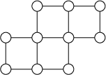
There exist numerous fields in which decomposing a tensor into a sum of rank-one terms is useful. These fields range from arithmetic complexity [12] to chemistry [54]. One nice application is worth to be emphasized, namely wireless transmissions [53]: one or several signals are wished to be extracted form noisy measurements, received on an array of sensors and disturbed by interferences. The approach is deterministic, which makes the difference compared to approaches based on data statistics [22]. The array of sensors is composed of JJ subarrays, each containing II sensors. Subarrays do not need to be disjoint, but must be deduced from each other by a translation in space. If the transmission is narrow band and in the far field, then the measurements at time sample tt recorded on sensor ii of subarray jj take the form:

T⁡(i,j,t)=∑p=1rAi​p​Bj​p​Ct​pT(i,j,t)=\sum_{p=1}^{r}A_{ip}B_{jp}C_{tp}

if rr waves impinge on the array. Matrices AA and BB characterize the geometry of the array (subarray and translations), whereas matrix CC contains the signals received on the array. An example with (I,J)=(4,4)(I,J)=(4,4) is given in Figure 1. Computing the decomposition of tensor TT allows to extract signals of interest as well as interferences, all included in matrix CC. Radiating sources can also be localized with the help of matrix AA if the exact location of sensors of a subarray are known. Note that this framework applies in radar, sonar or telecommunications.
Refer to caption
Figure 1. Array of 10 sensors decomposed into 4 subarrays of 4 sensors each.

4.1. Best approximation of lower multilinear rank

By considering a kkth order tensor as a linear map from one linear space onto the tensor product of the others, one can define the iith mode rank, which is nothing else but the rank of that linear operator. Since there are kk distinct possibilities to build such a linear operator, one defines a kk-uplet of ranks (r1,…​rk)(r_{1},\dots r_{k}), called the multilinear rank of the kkth order tensor. It is known that tensor rank is bounded below by all mode ranks rir_{i}:

(16) r≥ri,∀1≤i≤kr\geq r_{i},\forall 1\leq i\leq k

This inequality gives us an easily accessible lower bound. Let’s turn now to an upper bound.

Proposition 4.1.

[3] The rank of a tensor of order 3 and dimensions n1×n2×n3n_{1}\times n_{2}\times n_{3}, with n1≤n2n_{1}\leq n_{2}, is bounded by

(17) r≤n1+n2​⌊n3/2⌋r\leq n_{1}+n_{2}\lfloor n_{3}/2\rfloor

This bound on maximal rank has not been proved to be always reached, and it is likely to be quite loose for large values of nin_{i}. Nevertheless, it is sufficient for our reasoning.

There are two issues to address. First, the algorithm we have proposed is not usable in large dimensions (e.g. significantly larger than 10). The idea is then to reduce dimensions nin_{i} down to rir_{i} before executing the algorithm, if necessary. Second, another problem in practice is the presence of measurement errors or modeling inaccuracies, which increase the tensor rank to its generic value. We do not know how to reduce tensor rank back to its exact value. The practical solution is then to compute the best approximate of lower multilinear rank (r1,…​rk)(r_{1},\dots r_{k}), as explained in [23]. This best approximate always exists, and inequality (17) shows that reducing dimensions will indirectly reduce tensor rank. To compute it, it suffices to minimize ‖T−(U(1),U(2),U(3))⋅C‖||T-(U^{(1)},U^{(2)},U^{(3)})\cdot C|| with respect to the three matrices U(i)U^{(i)}, each of size ni×rin_{i}\times r_{i}, under the constraint U(1)​𝖧​U(1)=IU^{(1)\sf H}U^{(1)}=I. If properly initialized by a truncated HOSVD, a few iterations of any iterative algorithm will do it [46]. The tensor of reduced dimensions is then given by C=(U(1)​𝖧,U(2)​𝖧,U(3)​𝖧)⋅TC=(U^{(1)\sf H},U^{(2)\sf H},U^{(3)\sf H})\cdot T.

4.2. Number of solutions

In the above mentioned applications, it is necessary to have either a unique solution, or a finite set of solutions from which the most realistic one can be picked up. For this reason, it is convenient to make sure that the tensor rank is not too large, as pointed out by the following propositions.

Proposition 4.2.

[17] A generic symmetric tensor of order k≥3k\geq 3 and rank rr admits a finite number of decompositions into a sum of rank one terms if r<rE​(k,n)r<r_{E}(k,n), where:

(18) rE​(k,n)=⌈(n+k−1d)n⌉r_{E}(k,n)=\left\lceil\frac{\binom{n+k-1}{d}}{n}\right\rceil

Rank rEr_{E} is usually referred to as the expected rank of order kk and dimension nn.

Note that this result is true for generic tensors of rank rr, which means that there exists a set of exceptions, of null measure.

This proposition has not yet been entirely extended to unconstrained tensors, which we are interested in. However, some partial results are available in the literature [1], and the following conjecture is generally admitted

Conjecture 4.3.

A generic tensor of order k≥3k\geq 3 and rank rr admits a finite number of decompositions into a sum of rank one terms if r<rE​(k,𝐧)r<r_{E}(k,\mathbf{n}), where:

(19) rE​(k,𝐧)=⌈∏i=1kn11−k+∑i=1kni⌉r_{E}(k,\mathbf{n})=\left\lceil\frac{\prod_{i=1}^{k}n_{1}}{1-k+\sum_{i=1}^{k}n_{i}}\right\rceil

where nin_{i} denote the dimensions, 1≤i≤k1\leq i\leq k

On the other hand, a sufficient condition for uniqueness has been proposed by Kruskal [39], but the bound is more restrictive:

Proposition 4.4.

[39] A tensor of order k≥3k\geq 3 and rank rr admits a finite number of decompositions into a sum of rank one terms if:

(20) r≤∑i=1kκi2−1r\leq\frac{\sum_{i=1}^{k}\kappa_{i}}{2}-1

where κi\kappa_{i} denote the so-called Kruskal’s ranks of loading matrices, which generically equal the dimensions nin_{i} if the rank rr is larger than the latter.

4.3. Computer results

If we consider a 4×4×74\times 4\times 7 unconstrained tensor, it has an expected rank equal to 9, whereas Kruskal’s bound generically equals 6. So it is interesting to consider a tensor with such dimensions but with rank 6<r<96<r<9. In such conditions, we expect that there are almost surely a finite number of solutions. This tensor would correspond to measurements received on the array depicted in Figure 1, if 77 time samples are recorded. In [18] L. Chiantini and G. Ottaviani claim that a computer check shows that for a generic 4×4×74\times 4\times 7 tensor of rank 77, uniqueness of the decomposition holds.

Our computer results have been obtained with 4×4×74\times 4\times 7 tensors of rank 7 randomly drawn according to a continuous probability distribution.

First we consider a 4×4×44\times 4\times 4 tensor whose affine representation is given by:
T:=4+7​a1+8​a2+9​a3+5​b1−2​b2+11​b3+6​c1+8​c2+6​c3+21​a1​b1+28​a2​b1+11​a3​b1−14​a1​b2−21​a2​b2−10​a3​b2+48​a1​b3+65​a2​b3+28​a3​b3+26​a1​c1+35​a2​c1+14​a3​c1+18​b1​c1−10​b2​c1+40​b3​c1+36​a1​c2+48​a2​c2+18​a3​c2+26​b1​c2−9​b2​c2+55​b3​c2+38​a1​c3+53​a2​c3+14​a3​c3+26​b1​c3−16​b2​c3+58​b3​c3+68​a1​b1​c1+91​a2​b1​c1+48​a3​b1​c1−72​a1​b2​c1−105​a2​b2​c1−36​a3​b2​c1+172​a1​b3​c1+235​a2​b3​c1+112​a3​b3​c1+90​a1​b1​c2+118​a2​b1​c2+68​a3​b1​c2−85​a1​b2​c2−127​a2​b2​c2−37​a3​b2​c2+223​a1​b3​c2+301​a2​b3​c2+151​a3​b3​c2+96​a1​b1​c3+129​a2​b1​c3+72​a3​b1​c3−114​a1​b2​c3−165​a2​b2​c3−54​a3​b2​c3+250​a1​b3​c3+343​a2​b3​c3+166​a3​b3​c3.T:=4+7\,a_{1}+8\,a_{2}+9\,a_{3}+5\,b_{1}-2\,b_{2}+11\,b_{3}+6\,c_{1}+8\,c_{2}+6\,c_{3}+21\,a_{1}\,b_{1}+28\,a_{2}\,b_{1}+11\,a_{3}\,b_{1}-14\,a_{1}\,b_{2}-21\,a_{2}\,b_{2}-10\,a_{3}\,b_{2}+48\,a_{1}\,b_{3}+65\,a_{2}\,b_{3}+28\,a_{3}\,b_{3}+26\,a_{1}\,c_{1}+35\,a_{2}\,c_{1}+14\,a_{3}\,c_{1}+18\,b_{1}\,c_{1}-10\,b_{2}\,c_{1}+40\,b_{3}\,c_{1}+36\,a_{1}\,c_{2}+48\,a_{2}\,c_{2}+18\,a_{3}\,c_{2}+26\,b_{1}\,c_{2}-9\,b_{2}\,c_{2}+55\,b_{3}\,c_{2}+38\,a_{1}\,c_{3}+53\,a_{2}\,c_{3}+14\,a_{3}\,c_{3}+26\,b_{1}\,c_{3}-16\,b_{2}\,c_{3}+58\,b_{3}\,c_{3}+68\,a_{1}\,b_{1}\,c_{1}+91\,a_{2}\,b_{1}\,c_{1}+48\,a_{3}\,b_{1}\,c_{1}-72\,a_{1}\,b_{2}\,c_{1}-105\,a_{2}\,b_{2}\,c_{1}-36\,a_{3}\,b_{2}\,c_{1}+172\,a_{1}\,b_{3}\,c_{1}+235\,a_{2}\,b_{3}\,c_{1}+112\,a_{3}\,b_{3}\,c_{1}+90\,a_{1}\,b_{1}\,c_{2}+118\,a_{2}\,b_{1}\,c_{2}+68\,a_{3}\,b_{1}\,c_{2}-85\,a_{1}\,b_{2}\,c_{2}-127\,a_{2}\,b_{2}\,c_{2}-37\,a_{3}\,b_{2}\,c_{2}+223\,a_{1}\,b_{3}\,c_{2}+301\,a_{2}\,b_{3}\,c_{2}+151\,a_{3}\,b_{3}\,c_{2}+96\,a_{1}\,b_{1}\,c_{3}+129\,a_{2}\,b_{1}\,c_{3}+72\,a_{3}\,b_{1}\,c_{3}-114\,a_{1}\,b_{2}\,c_{3}-165\,a_{2}\,b_{2}\,c_{3}-54\,a_{3}\,b_{2}\,c_{3}+250\,a_{1}\,b_{3}\,c_{3}+343\,a_{2}\,b_{3}\,c_{3}+166\,a_{3}\,b_{3}\,c_{3}.

If we consider B′:=(1,b1,b2,b3)B^{\prime}:=(1,b_{1},b_{2},b_{3}) and B:=(1,a1,a2,a3)B:=(1,a_{1},a_{2},a_{3}), the corresponding matrix ℍΛB′,B\mathbb{H}_{\Lambda}^{B^{\prime},B} is equal to

ℍΛB′,B=(47895212811−2−14−21−1011486528)\mathbb{H}_{\Lambda}^{B^{\prime},B}=\left(\begin{array}[]{cccc}4&7&8&9\\ 5&21&28&11\\ -2&-14&-21&-10\\ 11&48&65&28\\ \end{array}\right)

and is invertible. Moreover, the transposed operators of multiplication by the variables c1,c2,c3c_{1},c_{2},c_{3} are known:

𝕄Bc1t=(011/6−2/3−1/6−2−41/620/319/6−2−85/637/329/6−25/201/2){}^{t}\mathbb{M}_{c_{1}}^{B}=\left(\begin{array}[]{cccc}0&11/6&-2/3&-1/6\\ -2&-41/6&20/3&19/6\\ -2&-85/6&37/3&29/6\\ -2&5/2&0&1/2\\ \end{array}\right)
𝕄Bc2t=(−223/3−13/3−1/3−61/37/313/3−6−28/329/320/3−614−70){}^{t}\mathbb{M}_{c_{2}}^{B}=\left(\begin{array}[]{cccc}-2&23/3&-13/3&-1/3\\ -6&1/3&7/3&13/3\\ -6&-28/3&29/3&20/3\\ -6&14&-7&0\\ \end{array}\right)
𝕄Bc3t=(03/20−1/2−2−33/21411/2−2−57/22317/2−23/22−1/2){}^{t}\mathbb{M}_{c_{3}}^{B}=\left(\begin{array}[]{cccc}0&3/2&0&-1/2\\ -2&-33/2&14&11/2\\ -2&-57/2&23&17/2\\ -2&3/2&2&-1/2\\ \end{array}\right)

whose eigenvalues are respectively (−1,2,4,1)(-1,2,4,1), (−2,4,5,1)(-2,4,5,1) and (−3,2,6,1)(-3,2,6,1). The corresponding common eigenvectors are:

v1=(1−1−23),v2=(1222),v3=(1573),v4=(1111).v_{1}=\left(\begin{array}[]{c}1\\ -1\\ -2\\ 3\\ \end{array}\right),v_{2}=\left(\begin{array}[]{c}1\\ 2\\ 2\\ 2\\ \end{array}\right),v_{3}=\left(\begin{array}[]{c}1\\ 5\\ 7\\ 3\\ \end{array}\right),v_{4}=\left(\begin{array}[]{c}1\\ 1\\ 1\\ 1\\ \end{array}\right).

We deduce that the coordinates (a1,a2,a3,b1,b2,b3,c1,c2,c3)(a_{1},a_{2},a_{3},b_{1},b_{2},b_{3},c_{1},c_{2},c_{3}) of the 4 points of evaluation are:

ζ1:=(−1−23???−1−2−3),ζ2:=(222???242),ζ3:=(573???456),ζ4:=(111???111),\zeta_{1}:=\left(\begin{array}[]{c}-1\\ -2\\ 3\\ ?\\ ?\\ ?\\ -1\\ -2\\ -3\\ \end{array}\right),\zeta_{2}:=\left(\begin{array}[]{c}2\\ 2\\ 2\\ ?\\ ?\\ ?\\ 2\\ 4\\ 2\\ \end{array}\right),\zeta_{3}:=\left(\begin{array}[]{c}5\\ 7\\ 3\\ ?\\ ?\\ ?\\ 4\\ 5\\ 6\\ \end{array}\right),\zeta_{4}:=\left(\begin{array}[]{c}1\\ 1\\ 1\\ ?\\ ?\\ ?\\ 1\\ 1\\ 1\\ \end{array}\right),

Then, computing the same way the operators of multiplication t𝕄c1B′,t𝕄c2B′,t𝕄c3B′{}^{t}\mathbb{M}_{c_{1}}^{B^{\prime}},^{t}\mathbb{M}_{c_{2}}^{B^{\prime}},^{t}\mathbb{M}_{c_{3}}^{B^{\prime}} and their common eigenvectors, we deduce:

ζ1=(−1−23−1−1−1−1−2−3),ζ2:=(222223242),ζ3=(5733−48456),ζ4=(111111111).\zeta_{1}=\left(\begin{array}[]{c}-1\\ -2\\ 3\\ -1\\ -1\\ -1\\ -1\\ -2\\ -3\\ \end{array}\right),\zeta_{2}:=\left(\begin{array}[]{c}2\\ 2\\ 2\\ 2\\ 2\\ 3\\ 2\\ 4\\ 2\\ \end{array}\right),\zeta_{3}=\left(\begin{array}[]{c}5\\ 7\\ 3\\ 3\\ -4\\ 8\\ 4\\ 5\\ 6\\ \end{array}\right),\zeta_{4}=\left(\begin{array}[]{c}1\\ 1\\ 1\\ 1\\ 1\\ 1\\ 1\\ 1\\ 1\\ \end{array}\right).

Finally, we have to solve the following linear system in (γ1,γ2,γ3,γ4)(\gamma_{1},\gamma_{2},\gamma_{3},\gamma_{4}):

T=γ1​(1+a1+a2+a3)​(1+b1+b2+b3)​(1+c1+c2+c3)+γ2​(1−a1−2​a2+3​a3)​(1−b1−b2−b3)​(1−c1−2​c2−3​c3)+γ3​(1+2​a1+2​a2+2​a3)​(1+2​b1+2​b2+3​b3)​(1+2​c1+4​c2+2​c3)+γ4​(1+5​a1+7​a2+3​a3)​(1+3​b1−4​b2+8​b3)​(1+4​c1+5​c2+6​c3)T=\gamma_{1}\,(1+a_{1}+a_{2}+a_{3})\,(1+b_{1}+b_{2}+b_{3})\,(1+c_{1}+c_{2}+c_{3})\\ +\gamma_{2}\,(1-a_{1}-2\,a_{2}+3\,a_{3})\,(1-b_{1}-b_{2}-b_{3})\,(1-c_{1}-2\,c_{2}-3\,c_{3})\\ +\gamma_{3}\,(1+2\,a_{1}+2\,a_{2}+2\,a_{3})\,(1+2\,b_{1}+2\,b_{2}+3\,b_{3})\,(1+2\,c_{1}+4\,c_{2}+2\,c_{3})\\ +\gamma_{4}\,(1+5\,a_{1}+7\,a_{2}+3\,a_{3})\,(1+3\,b_{1}-4\,b_{2}+8\,b_{3})\,(1+4\,c_{1}+5\,c_{2}+6\,c_{3}),
We get γ1=γ2=γ3=γ4=1\gamma_{1}=\gamma_{2}=\gamma_{3}=\gamma_{4}=1.
We consider such an example with 66 time samples, that is an element of ℝ4⊗ℝ4⊗ℝ6\mathbb{R}^{4}\otimes\mathbb{R}^{4}\otimes\mathbb{R}^{6}: T:=T:= 1046​a1​b1​c1+959​a1​b1​c2+660​a1​b1​c3+866​a1​b1​c4+952​a1​b1​c5−1318​a1​b2​c1−1222​a1​b2​c2−906​a1​b2​c3−1165​a1​b2​c4−1184​a1​b2​c5−153​a1​b3​c1+52​a1​b3​c2+353​a1​b3​c3+354​a1​b3​c4+585​a1​b3​c5+852​a2​b1​c1+833​a2​b1​c2+718​a2​b1​c3+903​a2​b1​c4+828​a2​b1​c5−1068​a2​b2​c1−1060​a2​b2​c2−992​a2​b2​c3−1224​a2​b2​c4−1026​a2​b2​c5+256​a2​b3​c1+468​a2​b3​c2+668​a2​b3​c3+748​a2​b3​c4+1198​a2​b3​c5−614​a3​b1​c1−495​a3​b1​c2−276​a3​b1​c3−392​a3​b1​c4−168​a3​b1​c5+664​a3​b2​c1+525​a3​b2​c2+336​a3​b2​c3+472​a3​b2​c4+63​a3​b2​c5+713​a3​b3​c1+737​a3​b3​c2+791​a3​b3​c3+965​a3​b3​c4+674​a3​b3​c5−95​a1​b1+88​a1​b2+193​a1​b3+320​a1​c1+285​a1​c2+134​a1​c3+188​a1​c4+382​a1​c5−29​a2​b1−2​a2​b2+198​a2​b3+292​a2​c1+269​a2​c2+138​a2​c3+187​a2​c4+406​a2​c5+119​a3​b1−139​a3​b2+20​a3​b3−222​a3​c1−160​a3​c2+32​a3​c3+9​a3​c4−229​a3​c5+122​b1​c1+119​b1​c2+112​b1​c3+140​b1​c4+108​b1​c5−160​b2​c1−163​b2​c2−176​b2​c3−214​b2​c4−117​b2​c5+31​b3​c1+57​b3​c2+65​b3​c3+73​b3​c4+196​b3​c5−35​a1−21​a2+54​a3−3​b1−3​b2+24​b3+50​c1+46​c2+20​c3+29​c4+63​c5−6.1046\,a_{1}\,b_{1}\,c_{1}+959\,a_{1}\,b_{1}\,c_{2}+660\,a_{1}\,b_{1}\,c_{3}+866\,a_{1}\,b_{1}\,c_{4}+952\,a_{1}\,b_{1}\,c_{5}-1318\,a_{1}\,b_{2}\,c_{1}-1222\,a_{1}\,b_{2}\,c_{2}-906\,a_{1}\,b_{2}\,c_{3}-1165\,a_{1}\,b_{2}\,c_{4}-1184\,a_{1}\,b_{2}\,c_{5}-153\,a_{1}\,b_{3}\,c_{1}+52\,a_{1}\,b_{3}\,c_{2}+353\,a_{1}\,b_{3}\,c_{3}+354\,a_{1}\,b_{3}\,c_{4}+585\,a_{1}\,b_{3}\,c_{5}+852\,a_{2}\,b_{1}\,c_{1}+833\,a_{2}\,b_{1}\,c_{2}+718\,a_{2}\,b_{1}\,c_{3}+903\,a_{2}\,b_{1}\,c_{4}+828\,a_{2}\,b_{1}\,c_{5}-1068\,a_{2}\,b_{2}\,c_{1}-1060\,a_{2}\,b_{2}\,c_{2}-992\,a_{2}\,b_{2}\,c_{3}-1224\,a_{2}\,b_{2}\,c_{4}-1026\,a_{2}\,b_{2}\,c_{5}+256\,a_{2}\,b_{3}\,c_{1}+468\,a_{2}\,b_{3}\,c_{2}+668\,a_{2}\,b_{3}\,c_{3}+748\,a_{2}\,b_{3}\,c_{4}+1198\,a_{2}\,b_{3}\,c_{5}-614\,a_{3}\,b_{1}\,c_{1}-495\,a_{3}\,b_{1}\,c_{2}-276\,a_{3}\,b_{1}\,c_{3}-392\,a_{3}\,b_{1}\,c_{4}-168\,a_{3}\,b_{1}\,c_{5}+664\,a_{3}\,b_{2}\,c_{1}+525\,a_{3}\,b_{2}\,c_{2}+336\,a_{3}\,b_{2}\,c_{3}+472\,a_{3}\,b_{2}\,c_{4}+63\,a_{3}\,b_{2}\,c_{5}+713\,a_{3}\,b_{3}\,c_{1}+737\,a_{3}\,b_{3}\,c_{2}+791\,a_{3}\,b_{3}\,c_{3}+965\,a_{3}\,b_{3}\,c_{4}+674\,a_{3}\,b_{3}\,c_{5}-95\,a_{1}\,b_{1}+88\,a_{1}\,b_{2}+193\,a_{1}\,b_{3}+320\,a_{1}\,c_{1}+285\,a_{1}\,c_{2}+134\,a_{1}\,c_{3}+188\,a_{1}\,c_{4}+382\,a_{1}\,c_{5}-29\,a_{2}\,b_{1}-2\,a_{2}\,b_{2}+198\,a_{2}\,b_{3}+292\,a_{2}\,c_{1}+269\,a_{2}\,c_{2}+138\,a_{2}\,c_{3}+187\,a_{2}\,c_{4}+406\,a_{2}\,c_{5}+119\,a_{3}\,b_{1}-139\,a_{3}\,b_{2}+20\,a_{3}\,b_{3}-222\,a_{3}\,c_{1}-160\,a_{3}\,c_{2}+32\,a_{3}\,c_{3}+9\,a_{3}\,c_{4}-229\,a_{3}\,c_{5}+122\,b_{1}\,c_{1}+119\,b_{1}\,c_{2}+112\,b_{1}\,c_{3}+140\,b_{1}\,c_{4}+108\,b_{1}\,c_{5}-160\,b_{2}\,c_{1}-163\,b_{2}\,c_{2}-176\,b_{2}\,c_{3}-214\,b_{2}\,c_{4}-117\,b_{2}\,c_{5}+31\,b_{3}\,c_{1}+57\,b_{3}\,c_{2}+65\,b_{3}\,c_{3}+73\,b_{3}\,c_{4}+196\,b_{3}\,c_{5}-35\,a_{1}-21\,a_{2}+54\,a_{3}-3\,b_{1}-3\,b_{2}+24\,b_{3}+50\,c_{1}+46\,c_{2}+20\,c_{3}+29\,c_{4}+63\,c_{5}-6.

If we take B={1,a1,a2,a3,b1,b2}B=\{1,a_{1},a_{2},a_{3},b_{1},b_{2}\} and B′={1,c1,c2,c3B^{\prime}=\{1,c_{1},c_{2},c_{3}, c4,c5}c_{4},c_{5}\} we obtain the following known submatrix of HΛH_{\Lambda}:

ℍΛB′,B=[−6−35−2154−3−350320292−222122−16046285269−160119−1632013413832112−176291881879140−21463382406−229108−117]\mathbb{H}^{B^{\prime},B}_{\Lambda}=\left[\begin{array}[]{cccccc}-6&-35&-21&54&-3&-3\\ \vskip 6.0pt plus 2.0pt minus 2.0pt\cr 50&320&292&-222&122&-160\\ \vskip 6.0pt plus 2.0pt minus 2.0pt\cr 46&285&269&-160&119&-163\\ \vskip 6.0pt plus 2.0pt minus 2.0pt\cr 20&134&138&32&112&-176\\ \vskip 6.0pt plus 2.0pt minus 2.0pt\cr 29&188&187&9&140&-214\\ \vskip 6.0pt plus 2.0pt minus 2.0pt\cr 63&382&406&-229&108&-117\end{array}\right]

which is invertible. Thus, the rank is at least 66. Let us find if HΛ~H_{\tilde{\Lambda}} can be extended to a rank 66 Hankel matrix HΛH_{\Lambda}. If we look at HΛB′⁣+,B+H^{B^{\prime+},B^{+}}_{\Lambda}, several coefficients are unknown. Yet, as will see, they can be determined by exploiting the commutation relations, as follows.

The columns ℍB′,{m}\mathbb{H}^{B^{\prime},\{m\}} are also known for m∈{b3,a1b1m\in\{b_{3},a_{1}\,b_{1}, a2b1,a3b1,a1b2,a2b2,a3b2}a_{2}\,b_{1},a_{3}\,b_{1},a_{1}\,b_{2},a_{2}\,b_{2},a_{3}\,b_{2}\}. Thus we deduce the relations between these monomials and BB by solving the system

ℍΛB′,B​X=ℍΛB′,{m}.\mathbb{H}^{B^{\prime},B}_{\Lambda}X=\mathbb{H}^{B^{\prime},\{m\}}_{\Lambda}.

This yields the following relations in 𝒜Λ\mathcal{A}_{\Lambda}:
b3≡−1.−0.02486​a1+1.412​a2+0.8530​a3−0.6116​b1+0.3713​b2,a1​b1≡−2.+6.122​a1−3.304​a2+.6740​a3+.7901​b1−1.282​b2,a2​b1≡−2.+4.298​a1−1.546​a2+1.364​a3+.5392​b1−1.655​b2,a3​b1≡−2.−3.337​a1+5.143​a2+1.786​a3−2.291​b1+1.699​b2,a1​b2≡−2.+0.03867​a1−0.1967​a2+1.451​a3−2.049​b1+3.756​b2,a2​b2≡−2.+3.652​a1−3.230​a2+.9425​a3−2.562​b1+4.198​b2,a3​b2≡−2.+6.243​a1−7.808​a2−1.452​a3+5.980​b1+0.03646​b2b_{3}\equiv-1.-0.02486\,a_{1}+1.412\,a_{2}+0.8530\,a_{3}-0.6116\,b_{1}+0.3713\,b_{2},a_{1}\,b_{1}\equiv-2.+6.122\,a_{1}-3.304\,a_{2}+.6740\,a_{3}+.7901\,b_{1}-1.282\,b_{2},a_{2}\,b_{1}\equiv-2.+4.298\,a_{1}-1.546\,a_{2}+1.364\,a_{3}+.5392\,b_{1}-1.655\,b_{2},a_{3}\,b_{1}\equiv-2.-3.337\,a_{1}+5.143\,a_{2}+1.786\,a_{3}-2.291\,b_{1}+1.699\,b_{2},a_{1}\,b_{2}\equiv-2.+0.03867\,a_{1}-0.1967\,a_{2}+1.451\,a_{3}-2.049\,b_{1}+3.756\,b_{2},a_{2}\,b_{2}\equiv-2.+3.652\,a_{1}-3.230\,a_{2}+.9425\,a_{3}-2.562\,b_{1}+4.198\,b_{2},a_{3}\,b_{2}\equiv-2.+6.243\,a_{1}-7.808\,a_{2}-1.452\,a_{3}+5.980\,b_{1}+0.03646\,b_{2}

Using the first relation on b3b_{3}, we can reduce a1​b3,a2​b3,a3​b3a_{1}\,b_{3},a_{2}\,b_{3},a_{3}\,b_{3} and obtain 33 linear dependency relations between the monomials in B∪{a12,a1​a2,a1​a3,a22,a2​a3,a32}B\cup\{a_{1}^{2},a_{1}a_{2},a_{1}a_{3},a_{2}^{2},a_{2}a_{3},a_{3}^{2}\}. Using the commutation relations lcm⁡(m1,m2)m1​N​(m1)−lcm⁡(m1,m2)m2​N​(m2){\mathrm{lcm}(m_{1},m_{2})\over m_{1}}N(m_{1})-{\mathrm{lcm}(m_{1},m_{2})\over m_{2}}N(m_{2}), for (m1,m2)∈{(a1b1,a2b1)(m_{1},m_{2})\in\{(a_{1}\,b_{1},a_{2}\,b_{1}), (a1b2,a2b2),(a2b2,a3b2)}(a_{1}\,b_{2},a_{2}\,b_{2}),(a_{2}\,b_{2},a_{3}\,b_{2})\} where N⁡(mi)N(m_{i}) is the reduction of mim_{i} with respect to the prevision relations, we obtain 33 new linear dependency relations between the monomials in B∪{a12,a1​a2,a1​a3,a22,a2​a3,a32}B\cup\{a_{1}^{2},a_{1}a_{2},a_{1}a_{3},a_{2}^{2},a_{2}a_{3},a_{3}^{2}\}. From these 66 relations, we deduce the expression of the monomials in {a12,a1a2,a1a3\{a_{1}^{2},a_{1}a_{2},a_{1}a_{3}, a22,a2a3,a32}a_{2}^{2},a_{2}a_{3},a_{3}^{2}\} as linear combinations of monomials in BB:
a12≡12.08a1−5.107a2+.2232a3−2.161b1−2.038b2−2.,a1a2≡8.972a1−1.431a2+1.392a3−3.680b1−2.254b2−2.,a1a3≡−11.56a1+9.209a2+2.802a3+1.737b1+.8155b2−2.,a22≡−2.+6.691a1+2.173a2+2.793a3−5.811b1−2.846b2,a2a3≡−2.−11.87a1+9.468a2+2.117a3+3.262b1+0.01989b2,a32≡−2.+16.96a1−8.603a2+1.349a3−6.351b1−.3558b2.a_{1}^{2}\equiv 12.08\,a_{1}-5.107\,a_{2}+.2232\,a_{3}-2.161\,b_{1}-2.038\,b_{2}-2.,a_{1}\,a_{2}\equiv 8.972\,a_{1}-1.431\,a_{2}+1.392\,a_{3}-3.680\,b_{1}-2.254\,b_{2}-2.,a_{1}\,a_{3}\equiv-11.56\,a_{1}+9.209\,a_{2}+2.802\,a_{3}+1.737\,b_{1}+.8155\,b_{2}-2.,a_{2}^{2}\equiv-2.+6.691\,a_{1}+2.173\,a_{2}+2.793\,a_{3}-5.811\,b_{1}-2.846\,b_{2},a_{2}\,a_{3}\equiv-2.-11.87\,a_{1}+9.468\,a_{2}+2.117\,a_{3}+3.262\,b_{1}+0.01989\,b_{2},a_{3}^{2}\equiv-2.+16.96\,a_{1}-8.603\,a_{2}+1.349\,a_{3}-6.351\,b_{1}-.3558\,b_{2}.

Now, we are able to compute the matrix of multiplication by a1a_{1} in BB, which is obtained by reducing the monomials B⋅a1={a1,a12,a1​a2,a1​a3,a1​b1,a1​b2}B\cdot a_{1}=\{a_{1},a_{1}^{2},a_{1}\,a_{2},a_{1}\,a_{3},a_{1}\,b_{1},a_{1}\,b_{2}\} by the computed relations:

Ma1:=[0.0−2.0−2.0−2.0−2.0−2.01.012.088.972−11.566.1220.038670.0−5.107−1.4319.209−3.304−0.19670.00.22321.3922.8020.67401.4510.0−2.161−3.6801.7370.7901−2.0490.0−2.038−2.2540.8155−1.2823.756].M_{a_{1}}:=\left[\begin{array}[]{cccccc}0.0&-2.0&-2.0&-2.0&-2.0&-2.0\\ \vskip 6.0pt plus 2.0pt minus 2.0pt\cr 1.0&12.08&8.972&-11.56&6.122&0.03867\\ \vskip 6.0pt plus 2.0pt minus 2.0pt\cr 0.0&-5.107&-1.431&9.209&-3.304&-0.1967\\ \vskip 6.0pt plus 2.0pt minus 2.0pt\cr 0.0&0.2232&1.392&2.802&0.6740&1.451\\ \vskip 6.0pt plus 2.0pt minus 2.0pt\cr 0.0&-2.161&-3.680&1.737&0.7901&-2.049\\ \vskip 6.0pt plus 2.0pt minus 2.0pt\cr 0.0&-2.038&-2.254&0.8155&-1.282&3.756\end{array}\right].

The eigenvectors of the transposed operator normalized so that the first coordinate is 11 are:

[1.05.07.0033.03.0−4.0],[1.02.9994.0−4.999−2.9994.999],[1.02.02.02.02.02.0],[1.08.0016.002−7.0024.001−5.001],[1.0−1.0−2.03.0−1.0−1.0],[1.00.99990.99990.99990.99990.9999]\left[\begin{array}[]{c}1.0\\ \vskip 6.0pt plus 2.0pt minus 2.0pt\cr 5.0\\ \vskip 6.0pt plus 2.0pt minus 2.0pt\cr 7.003\\ \vskip 6.0pt plus 2.0pt minus 2.0pt\cr 3.0\\ \vskip 6.0pt plus 2.0pt minus 2.0pt\cr 3.0\\ \vskip 6.0pt plus 2.0pt minus 2.0pt\cr-4.0\end{array}\right],\left[\begin{array}[]{c}1.0\\ \vskip 6.0pt plus 2.0pt minus 2.0pt\cr 2.999\\ \vskip 6.0pt plus 2.0pt minus 2.0pt\cr 4.0\\ \vskip 6.0pt plus 2.0pt minus 2.0pt\cr-4.999\\ \vskip 6.0pt plus 2.0pt minus 2.0pt\cr-2.999\\ \vskip 6.0pt plus 2.0pt minus 2.0pt\cr 4.999\end{array}\right],\left[\begin{array}[]{c}1.0\\ \vskip 6.0pt plus 2.0pt minus 2.0pt\cr 2.0\\ \vskip 6.0pt plus 2.0pt minus 2.0pt\cr 2.0\\ \vskip 6.0pt plus 2.0pt minus 2.0pt\cr 2.0\\ \vskip 6.0pt plus 2.0pt minus 2.0pt\cr 2.0\\ \vskip 6.0pt plus 2.0pt minus 2.0pt\cr 2.0\end{array}\right],\left[\begin{array}[]{c}1.0\\ \vskip 6.0pt plus 2.0pt minus 2.0pt\cr 8.001\\ \vskip 6.0pt plus 2.0pt minus 2.0pt\cr 6.002\\ \vskip 6.0pt plus 2.0pt minus 2.0pt\cr-7.002\\ \vskip 6.0pt plus 2.0pt minus 2.0pt\cr 4.001\\ \vskip 6.0pt plus 2.0pt minus 2.0pt\cr-5.001\end{array}\right],\left[\begin{array}[]{c}1.0\\ \vskip 6.0pt plus 2.0pt minus 2.0pt\cr-1.0\\ \vskip 6.0pt plus 2.0pt minus 2.0pt\cr-2.0\\ \vskip 6.0pt plus 2.0pt minus 2.0pt\cr 3.0\\ \vskip 6.0pt plus 2.0pt minus 2.0pt\cr-1.0\\ \vskip 6.0pt plus 2.0pt minus 2.0pt\cr-1.0\end{array}\right],\left[\begin{array}[]{c}1.0\\ \vskip 6.0pt plus 2.0pt minus 2.0pt\cr 0.9999\\ \vskip 6.0pt plus 2.0pt minus 2.0pt\cr 0.9999\\ \vskip 6.0pt plus 2.0pt minus 2.0pt\cr 0.9999\\ \vskip 6.0pt plus 2.0pt minus 2.0pt\cr 0.9999\\ \vskip 6.0pt plus 2.0pt minus 2.0pt\cr 0.9999\end{array}\right]

They correspond to the vectors of evaluation of the monomial vector BB at the roots of IΛI_{\Lambda}. Thus we known the coordinates a1,a2,a3,b1,b2a_{1},a_{2},a_{3},b_{1},b_{2} of these roots. By expanding the polynomial
OPENγ1​(1+a1+a2+a3))​(1+b1+b2+b3)​(1+⋯)+γ2​(1−a1−2​a2+3​a3)​(1−b1−b2−b3)​(1+⋯)+γ3​(1+2​a1+2​a2+2​a3)​(1+2​b1+2​b2+3​b3)​(1+⋯)+γ4​(1+5​a1+7​a2+3​a3)​(1+3​b1−4​b2+8​b3)​(1+⋯)+γ5​(1+8​a1+6​a2−7​a3)​(1+4​b1−5​b2−3​b3)​(1+⋯)+γ6​(1+3​a1+4​a2−5​a3)​(1−3​b1+5​b2+4​b3)​(1+⋯)\gamma_{1}\,(1+a_{1}+a_{2}+a_{3}))\,(1+b_{1}+b_{2}+b_{3})\,(1+\cdots)+\gamma_{2}\,(1-a_{1}-2\,a_{2}+3\,a_{3})\,(1-b_{1}-b_{2}-b_{3})\,(1+\cdots)+\gamma_{3}\,(1+2\,a_{1}+2\,a_{2}+2\,a_{3})\,(1+2\,b_{1}+2\,b_{2}+3\,b_{3})\,(1+\cdots)+\gamma_{4}\,(1+5\,a_{1}+7\,a_{2}+3\,a_{3})\,(1+3\,b_{1}-4\,b_{2}+8\,b_{3})\,(1+\cdots)+\gamma_{5}\,(1+8\,a_{1}+6\,a_{2}-7\,a_{3})\,(1+4\,b_{1}-5\,b_{2}-3\,b_{3})\,(1+\cdots)+\gamma_{6}\,(1+3\,a_{1}+4\,a_{2}-5\,a_{3})\,(1-3\,b_{1}+5\,b_{2}+4\,b_{3})\,(1+\cdots)
(where the ⋯\cdots are terms linear in cic_{i}) and identifying the coefficients of TT which do not depend on c1,…,c5c_{1},\ldots,c_{5}, we obtain a linear system in γi\gamma_{i}, which unique solution is (2,−1,−2,3CLOSE(2,-1,-2,3, OPEN−5,−3)-5,-3). This allows us to compute the value Λ\Lambda for any monomials in {a1,a2,a3,b1,b2,b3}\{a_{1},a_{2},a_{3},b_{1},b_{2},b_{3}\}. In particular, we can compute the entries of ℍΛB,B\mathbb{H}^{B,B}_{\Lambda}. Solving the system ℍΛB,B​X=ℍΛB,B′,\mathbb{H}^{B,B}_{\Lambda}\,X=\mathbb{H}^{B,B^{\prime}}_{\Lambda}, we deduce the relations between the monomials in B′B^{\prime} and BB in 𝒜Λ\mathcal{A}_{\Lambda} and in particular c1,…,c5c_{1},\ldots,c_{5} as linear combinations of monomials in BB. This allows us to recover the missing coordinates and yields the following decomposition:
T:=T:= 2​(1+a1+a2+a3)​(1+b1+b2+b3)​(1+c1+c2+c3+c4+c5)−(1−a1−2​a2+3​a3)​(1−b1−b2−b3)​(1−c1−2​c2−3​c3−4​c4+5​c5)−2​(1+2​a1+2​a2+2​a3)​(1+2​b1+2​b2+3​b3)​(1+2​c1+2​c2+2​c3+2​c4+2​c5)+3​(1+5​a1+7​a2+3​a3)​(1+3​b1−4​b2+8​b3)​(1+4​c1+5​c2+6​c3+7​c4+8​c5)−5​(1+8​a1+6​a2−7​a3)​(1+4​b1−5​b2−3​b3)​(1−6​c1−5​c2−2​c3−3​c4−5​c5)−3​(1+3​a1+4​a2−5​a3)​(1−3​b1+5​b2+4​b3)​(1−3​c1−2​c2+3​c3+3​c4−7​c5).2\,(1+a_{1}+a_{2}+a_{3})\,(1+b_{1}+b_{2}+b_{3})\,(1+c_{1}+c_{2}+c_{3}+c_{4}+c_{5})-(1-a_{1}-2\,a_{2}+3\,a_{3})\,(1-b_{1}-b_{2}-b_{3})\,(1-c_{1}-2\,c_{2}-3\,c_{3}-4\,c_{4}+5\,c_{5})-2\,(1+2\,a_{1}+2\,a_{2}+2\,a_{3})\,(1+2\,b_{1}+2\,b_{2}+3\,b_{3})\,(1+2\,c_{1}+2\,c_{2}+2\,c_{3}+2\,c_{4}+2\,c_{5})+3\,(1+5\,a_{1}+7\,a_{2}+3\,a_{3})\,(1+3\,b_{1}-4\,b_{2}+8\,b_{3})\,(1+4\,c_{1}+5\,c_{2}+6\,c_{3}+7\,c_{4}+8\,c_{5})-5\,(1+8\,a_{1}+6\,a_{2}-7\,a_{3})\,(1+4\,b_{1}-5\,b_{2}-3\,b_{3})\,(1-6\,c_{1}-5\,c_{2}-2\,c_{3}-3\,c_{4}-5\,c_{5})-3\,(1+3\,a_{1}+4\,a_{2}-5\,a_{3})\,(1-3\,b_{1}+5\,b_{2}+4\,b_{3})\,(1-3\,c_{1}-2\,c_{2}+3\,c_{3}+3\,c_{4}-7\,c_{5}).

References

  • [1] H. Abo, G. Ottaviani, and C. Peterson. Induction for secant varieties of Segre varieties. Trans. Amer. Math. Soc., pages 767–792, 2009. arXiv:math/0607191.
  • [2] E. S. Allman and J. A. Rhodes. Phylogenetic ideals and varieties for the general Markov model. Adv. in Appl. Math., 40(2):127–148, 2008.
  • [3] M. D. Atkinson and N. M. Stephens. On the maximal multiplicative complexity of a family of bilinear forms. Linear Algebra Appl., 27:1–8, October 1979.
  • [4] E. Ballico and A. Bernardi. Stratification of the fourth secant variety of veronese variety via symmetric rank. arXiv 1005.3465, 2010.
  • [5] A. Bernardi. Ideals of varieties parameterized by certain symmetric tensors. J. Pure Appl. Algebra, 212(6):1542–1559, 2008.
  • [6] A. Bernardi, J. Brachat, P. Comon, and B. Mourrain. Multihomogeneous polynomial decomposition using moment matrices. In A. Leykin, editor, International Symposium on Symbolic and Algebraic Computation (ISSAC), pages 35–42, San Jose, CA, United States, June 2011. ACM New York.
  • [7] A. Bernardi, A. Gimigliano, and M. Idà. Computing symmetric rank for symmetric tensors. J. Symb. Comput., 46:34–53, January 2011.
  • [8] D. Bini, M. Capovani, F. Romani, and G. Lotti. O⁡(n2.77)O(n^{2.77}) Complexity for n×nn\times n approximate matrix multiplication. Inform. Process, 8(5):234–235, 1979.
  • [9] J. Brachat, P. Comon, B. Mourrain, and E. Tsigaridas. Symmetric tensor decomposition. Linear Algebra and Applications, 433:1851–1872, 2010.
  • [10] R. Bro. Parafac, tutorial and applications. Chemom. Intel. Lab. Syst., 38:149–171, 1997.
  • [11] J. Buczynski, A. Ginensky, and J.M. Landsberg. Determinental equations for secant varieties and the Eisenbud-Koh-Stillman conjecture. 1007.0192, 2010.
  • [12] P. Bürgisser, M. Clausen, and M. A. Shokrollahi. Algebraic complexity theory, volume 315 of Grundlehren der Mathematischen Wissenschaften [Fundamental Principles of Mathematical Sciences]. Springer-Verlag, Berlin, 1997. With the collaboration of Thomas Lickteig.
  • [13] J. F. Cardoso. Blind signal separation: statistical principles. Proc. of the IEEE, 90:2009–2025, October 1998. special issue, R.W. Liu and L. Tong eds.
  • [14] M. V. Catalisano, A. V. Geramita, and A. Gimigliano. On the ideals of secant varieties to certain rational varieties. J. Algebra, 319(5):1913–1931, 2008.
  • [15] P. Chevalier. Optimal separation of independent narrow-band sources - concept and performance. Signal Processing, Elsevier, 73(1):27–48, February 1999. special issue on blind separation and deconvolution.
  • [16] P. Chevalier, L. Albera, A. Ferreol, and P. Comon. On the virtual array concept for higher order array processing. IEEE Proc., 53(4):1254–1271, April 2005.
  • [17] L. Chiantini and C. Ciliberto. Weakly defective varieties. Trans. of the Am. Math. Soc., 354(1):151–178, 2001.
  • [18] Luca Chiantini and Giorgio Ottaviani. On generic identifiability of 3-tensors of small rank. http://arxiv.org/abs/1103.2696, 03 2011.
  • [19] A. Cichocki and S-I. Amari. Adaptive Blind Signal and Image Processing. Wiley, New York, 2002.
  • [20] G. Comas and M. Seiguer. On the rank of a binary form, 2001.
  • [21] P. Comon. Independent Component Analysis. In J-L. Lacoume, editor, Higher Order Statistics, pages 29–38. Elsevier, Amsterdam, London, 1992.
  • [22] P. Comon and C. Jutten, editors. Handbook of Blind Source Separation, Independent Component Analysis and Applications. Academic Press, Oxford UK, Burlington USA, 2010.
  • [23] P. Comon, X. Luciani, and A. L. F. De Almeida. Tensor decompositions, alternating least squares and other tales. Jour. Chemometrics, 23:393–405, August 2009.
  • [24] P. Comon and B. Mourrain. Decomposition of quantics in sums of powers of linear forms. Signal Processing, 53(2-3):93–107, 1996.
  • [25] P. Comon and M. Rajih. Blind identification of under-determined mixtures based on the characteristic function. Signal Processing, 86(9):2271–2281, 2006.
  • [26] D. Cox, J. Little, and D. O’Shea. Ideals, Varieties, and Algorithms. Undergraduate Texts in Mathematics. Springer-Verlag, New York, 2nd edition, 1997.
  • [27] D. Cox, J. Little, and D. O’Shea. Using Algebraic Geometry. Number 185 in Graduate Texts in Mathematics. Springer, New York, 2nd edition, 2005.
  • [28] L. de Lathauwer and J. Castaing. Tensor-based techniques for the blind separation of ds-cdma signals. Signal Processing, 87(2):322–336, February 2007.
  • [29] M. C. Dogan and J. Mendel. Applications of cumulants to array processing .I. aperture extension and array calibration. IEEE Trans. Sig. Proc., 43(5):1200–1216, May 1995.
  • [30] D. L. Donoho and X. Huo. Uncertainty principles and ideal atomic decompositions. IEEE Trans. Inform. Theory, 47(7):2845–2862, November 2001.
  • [31] M. Elkadi and B. Mourrain. Introduction à la résolution des systèmes polynomiaux, volume 59 of Mathḿatiques et Applications. Springer, 2007.
  • [32] A. Ferreol and P. Chevalier. On the behavior of current second and higher order blind source separation methods for cyclostationary sources. IEEE Trans. Sig. Proc., 48:1712–1725, June 2000. erratum in vol.50, pp.990, Apr. 2002.
  • [33] A. V. Geramita. Catalecticant varieties. In Commutative algebra and algebraic geometry (Ferrara), volume 206 of Lecture Notes in Pure and Appl. Math., pages 143–156. Dekker, New York, 1999.
  • [34] R. Grone. Decomposable tensors as a quadratic variety. Proc. Amer. Math. Soc., 64(2):227–230, 1977.
  • [35] H. T. Hà. Box-shaped matrices and the defining ideal of certain blowup surfaces. J. Pure Appl. Algebra, 167(2-3):203–224, 2002.
  • [36] A. Iarrobino and V. Kanev. Power sums, Gorenstein algebras, and determinantal loci, volume 1721 of Lecture Notes in Computer Science. Springer-Verlag, Berlin, 1999.
  • [37] T. Jiang and N. Sidiropoulos. Kruskal’s permutation lemma and the identification of CANDECOMP/PARAFAC and bilinear models. IEEE Trans. Sig. Proc., 52(9):2625–2636, September 2004.
  • [38] H. A. L. Kiers and W. P. Krijnen. An efficient algorithm for Parafac of three-way data with large numbers of observation units. Psychometrika, 56:147, 1991.
  • [39] J. B. Kruskal. Three-way arrays: Rank and uniqueness of trilinear decompositions. Linear Algebra and Applications, 18:95–138, 1977.
  • [40] J. Landsberg. Geometry and the complexity of matrix multiplication. Bull. Amer. Math. Soc., 45(2):247–284, April 2008.
  • [41] J. M. Landsberg and L. Manivel. On the ideals of secant varieties of Segre varieties. Found. Comput. Math., 4(4):397–422, 2004.
  • [42] J. M. Landsberg and L. Manivel. Generalizations of Strassen’s equations for secant varieties of Segre varieties. Comm. Algebra, 36(2):405–422, 2008.
  • [43] J. M. Landsberg and G. Ottaviani. Equations for secant varieties to veronese varieties. arXiv 1006.0180, 2010.
  • [44] J. M. Landsberg and G. Ottaviani. Equations for secant varieties via vector bundles. arXiv 1010.1825, 2010.
  • [45] J. M. Landsberg and J. Weyman. On the ideals and singularities of secant varieties of Segre varieties. Bull. Lond. Math. Soc., 39(4):685–697, 2007.
  • [46] L. De Lathauwer, B. De Moor, and J. Vandewalle. On the best rank-1 and rank-(R1,R2,. . . RN) approximation of high-order tensors. SIAM Jour. Matrix Ana. Appl., 21(4):1324–1342, April 2000.
  • [47] M. Laurent and B. Mourrain. A Sparse Flat Extension Theorem for Moment Matrices. Archiv der Mathematik, 93:87–98, 2009.
  • [48] B. Mourrain. A new criterion for normal form algorithms. In M. Fossorier, H. Imai, S. Lin, and A. Poli, editors, Proc. Applic. Algebra in Engineering, Communic. and Computing, volume 1719 of Lecture Notes in Computer Science, pages 430–443. Springer, Berlin, 1999.
  • [49] B. Mourrain and V.Y. Pan. Multivariate Polynomials, Duality, and Structured Matrices. Journal of Complexity, 16(1):110–180, 2000.
  • [50] G. Ottaviani. An invariant regarding Waring’s problem for cubic polynomials. Nagoya Math. J., 193:95–110, 2009.
  • [51] A. Parolin. Varietà secanti alle varietà di segre e di veronese e loro applicazioni, tesi di dottorato. Università di Bologna, 2003/2004.
  • [52] M. Pucci. The Veronese variety and catalecticant matrices. J. Algebra, 202(1):72–95, 1998.
  • [53] N. D. Sidiropoulos, G. B. Giannakis, and R. Bro. Blind PARAFAC receivers for DS-CDMA systems. IEEE Trans. on Sig. Proc., 48(3):810–823, 2000.
  • [54] A. Smilde, R. Bro, and P. Geladi. Multi-Way Analysis. Wiley, 2004.
  • [55] V. Strassen. Rank and optimal computation of generic tensors. Linear Algebra Appl., 52:645–685, July 1983.
  • [56] A. Swami, G. Giannakis, and S. Shamsunder. Multichannel ARMA processes. IEEE Trans. Sig. Proc., 42(4):898–913, April 1994.
  • [57] J. J. Sylvester. Sur une extension d’un théorème de Clebsch relatif aux courbes du quatrième degré. Comptes Rendus, Math. Acad. Sci. Paris, 102:1532–1534, 1886.
  • [58] A. J. van der Veen and A. Paulraj. An analytical constant modulus algorithm. IEEE Trans. Sig. Proc., 44(5):1136–1155, May 1996.
  • [59] K. Wakeford. On canonical forms. Proc. London Math. Soc., 18:403–410, 1918-19.