Efficient Squares and Turing Universality at Temperature 1 with a Unique Negative Glue

We now give a brief and intuitive sketch of the Tile Assembly Model that is adequate for reading this paper. More formal details and discussion may be found in [22, 19, 18, 13].

Intuitively, a tile type $t$ is a unit square that can be translated, but not rotated, having a well-defined “side $\vec{u}$” for each $\vec{u}\in U_{2}$. Each side $\vec{u}$ of $t$ has a “glue” of “color” $\textmd{col}_{t}(\vec{u})$ – a string over some fixed alphabet $\Sigma$ – and “strength” $\textmd{str}_{t}(\vec{u})$–an integer–specified by its type $t$. Two tiles $t$ and $t^{\prime}$ that are placed at the points $\vec{a}$ and $\vec{a}+\vec{u}$, respectively, interact with strength $\textmd{str}_{t}\left(\vec{u}\right)$ if and only if $\left(\textmd{col}_{t}\left(\vec{u}\right),\textmd{str}_{t}\left(\vec{u}\right)\right)=\left(\textmd{col}_{t^{\prime}}\left(-\vec{u}\right),\textmd{str}_{t^{\prime}}\left(-\vec{u}\right)\right)$. If $\textmd{str}_{t}\left(\vec{u}\right)>0$, those tiles bind with that strength.

Given a set $T$ of tile types, an assembly is a partial function $\alpha:\mathbb{Z}^{2}\dashrightarrow T$, with points $\vec{x}\in\mathbb{Z}^{2}$ at which $\alpha(\vec{x})$ is undefined interpreted to be empty space, so that ${\rm dom}\;\alpha$ is the set of points with tiles. $\alpha$ is finite if $|{\rm dom}\;\alpha|$ is finite. For assemblies $\alpha$ and $\alpha^{\prime}$, we say that $\alpha$ is a subconfiguration of $\alpha^{\prime}$, and write $\alpha\sqsubseteq\alpha^{\prime}$, if ${\rm dom}\;\alpha\subseteq{\rm dom}\;\alpha^{\prime}$ and $\alpha(\vec{x})=\alpha^{\prime}(\vec{x})$ for all $x\in{\rm dom}\;\alpha$.

A grid graph is a graph $G=(V,E)$ in which $V\subseteq\mathbb{Z}^{2}$ and every edge $\{\vec{a},\vec{b}\}\in E$ has the property that $\vec{a}-\vec{b}\in U_{2}$. The binding graph of an assembly $\alpha$ is the grid graph $G_{\alpha}=(V,E)$, where $V={\rm dom}\;{\alpha}$, and $\{\vec{m},\vec{n}\}\in E$ if and only if (1) $\vec{m}-\vec{n}\in U_{2}$, (2) ${\rm col}_{\alpha(\vec{m})}\left(\vec{n}-\vec{m}\right)={\rm col}_{\alpha(\vec{n})}\left(\vec{m}-\vec{n}\right)$, (3) ${\rm str}_{\alpha(\vec{m})}\left(\vec{n}-\vec{m}\right)={\rm str}_{\alpha(\vec{n})}\left(\vec{m}-\vec{n}\right)$, and (4) ${\rm str}_{\alpha(\vec{m})}\left(\vec{n}-\vec{m}\right)>0$. An assembly is $\tau$-stable, where $\tau\in\mathbb{N}$, if it cannot be broken up into smaller assemblies without breaking bonds of total strength at least $\tau$ (i.e., if every cut of $G_{\alpha}$ cuts edges the sum of whose strengths is at least $\tau$). For the case of negative strength glues, we employ the model of irreversible assembly as defined in [6].

Self-assembly begins with a seed assembly $\sigma$ (typically assumed to be finite and $\tau$-stable) and proceeds asynchronously and nondeterministically, with tiles adsorbing one at a time to the existing assembly in any manner that preserves stability at all times.

A tile assembly system (TAS) is an ordered triple $\mathcal{T}=(T,\sigma,\tau)$, where $T$ is a finite set of tile types, $\sigma$ is a seed assembly with finite domain, and $\tau$ is the temperature. In subsequent sections of this paper, unless explicitly stated otherwise, we assume that $\tau=1$ and $\sigma$ consists of a single seed tile type placed at the origin. An assembly sequence in a TAS $\mathcal{T}=(T,\sigma,1)$ is a (possibly infinite) sequence $\vec{\alpha}=(\alpha_{i}\mid 0\leq i<k)$ of assemblies in which $\alpha_{0}=\sigma$ and each $\alpha_{i+1}$ is obtained from $\alpha_{i}$ by the “$\tau$-stable” addition of a single tile. The result of an assembly sequence $\vec{\alpha}$ is the unique assembly $\textrm{res}\left(\vec{\alpha}\right)$ satisfying ${\rm dom}\;{\textrm{res}\left(\vec{\alpha}\right)}=\bigcup_{0\leq i<k}{{\rm dom}\;{\alpha_{i}}}$ and, for each $0\leq i<k$, $\alpha_{i}\sqsubseteq\textrm{res}\left(\vec{\alpha}\right)$. If $\vec{\alpha}=\left(\alpha_{i}\mid 0\leq i<k\right)$ is an assembly sequence in $\mathcal{T}$ and $\vec{m}\in\mathbb{Z}^{2}$, then the $\vec{\alpha}$-index of $\vec{m}$ is $i_{\vec{\alpha}}(\vec{m})=\min\{i\in\mathbb{N}\;\left|\;\vec{m}\in{\rm dom}\;{\alpha_{i}}\right.\}$. That is, the $\vec{\alpha}$-index of $\vec{m}$ is the time at which any tile is first placed at location $\vec{m}$ by $\vec{\alpha}$. For each location $\vec{m}\in\bigcup_{0\leq i<l}{{\rm dom}\;{\alpha_{i}}}$, define the set of its input sides $\textmd{IN}^{\vec{\alpha}}(\vec{m})=\left\{\vec{u}\in U_{2}\;\left|\;\textmd{str}_{\alpha_{i_{\vec{\alpha}}(\vec{m})}}(\vec{u})>0\right.\right\}$.

We write $\mathcal{A}[\mathcal{T}]$ for the set of all producible assemblies of $\mathcal{T}$. An assembly $\alpha$ is terminal, and we write $\alpha\in\mathcal{A}_{\Box}[\mathcal{\mathcal{T}}]$, if no tile can be stably added to it. We write $\mathcal{A}_{\Box}[\mathcal{T}]$ for the set of all terminal assemblies of $\mathcal{T}$. A TAS ${\mathcal{T}}$ is directed, or produces a unique assembly, if it has exactly one terminal assembly i.e., $|\mathcal{A}_{\Box}[\mathcal{T}]|=1$. A set $X$ strictly self-assembles if there is a TAS $\mathcal{T}$ for which every assembly $\alpha\in\mathcal{A}_{\Box}[\mathcal{T}]$ satisfies ${\rm dom}\;\alpha=X$.

Restricted Glue Tile Assembly Systems.

We say that a tile set $T$ is glue restricted if (1) the absolute value of every glue strength in $T$ is 1, (2) the glue function is diagonal, meaning that for every glue type $g$, the interaction between $g$ and any other glue type is of strength $0$, and of magnitude $1$ between two copies of $g$, and (3) there is a single negative-strength glue type. Intuitively, glue restricted tile sets are as “close” as one can get to pure temperature one self-assembly in the aTAM. A TAS $\mathcal{T}=(T,\sigma,1)$ is glue restricted if $T$ is glue restricted. In this paper, for notational convenience, we will simply refer to a glue restricted TAS as an rgTAS.

Due to the potential difficulty of experimentally implementing negative strength glues such that the magnitude of their strengths is very nearly exactly equivalent to that of the positive strength-$1$ glues, we also introduce another type of tile assembly system, which we refer to as partially glue restricted tile assembly system, or prgTAS. A tile set in a prgTAS has the same properties as those for rgTASs, except for the fact that the magnitude of the strength of the single negative glue is guaranteed to be at least 1, but may in fact be greater (i.e. the effective glue strength could actually be $-2,-3,$ etc.).

Zig-zag tile assembly systems. A tile assembly system $\mathcal{T}=(T,\sigma,2)$ is called a zig-zag [4] tile assembly system if (1) $\mathcal{T}$ is directed, (2) there is a single assembly sequence $\vec{\alpha}$ in $\mathcal{T}$, with $\mathcal{A}_{\Box}[\mathcal{T}]=\{\alpha\}$, and (3) for every $\vec{x}\in{\rm dom}\;{\alpha}$, $(0,1)\not\in\textmd{IN}^{\vec{\alpha}}(\vec{x})$. Intuitively, zig-zag systems are those that grow one horizontal row at a time, alternating left-to-right and right-to-left growth, always adding new rows to the north and never growing south. Zig-zag systems are capable of simulating universal Turing machines, and thus universal computation [4]. If $\mathcal{T}$ is a zig-zag system with $\mathcal{A}_{\Box}[\mathcal{T}]=\{\alpha\}$ and for every $\vec{x}\in{\rm dom}\;{\alpha}$ and every $\vec{u}\in U_{2}$, $\textmd{str}_{\alpha(\vec{x})}(\vec{u})+\textmd{str}_{\alpha(\vec{x})}(-\vec{u})<4$, then we say that $\mathcal{T}$ is compact. Intuitively, compact zig-zag systems are zig-zag systems that only extend the width of each row by one over the length of the previous row, and only grow upward by one tile before continuing horizontal growth. Compact zig-zag systems are capable of simulating universal Turing machines [4].

Path simulation. Let $\mathcal{T}=(T,\sigma,2)$ be a zig-zag TAS with assembly sequence $\vec{\alpha}=(\alpha_{i}\mid 0\leq i<k)$. We say that a restricted TAS $\mathcal{S}=(S,\sigma,1)$ path simulates $\mathcal{T}$ (at scale factor $c$) if (1) $\mathcal{S}$ has a single assembly sequence, (2) there exist computable indices $0=i_{-1}<i_{0}<\cdots<i_{k-1}<i_{k}=k$ satisfying $c=\max\left\{\left.i_{j}-i_{j-1}\;\right|\;0\leq j<k\right\}$ and (3) there exists a computable function $f:\mathcal{A}[\mathcal{S}]\longrightarrow\mathcal{A}[\mathcal{T}]$ such that, for all $0\leq j<k$, $f\left(\textrm{res}\left(\left(\alpha_{i_{j-1}},\ldots,\alpha_{i_{j}-1}\right)\right)\right)=\alpha_{j}$. Intuitively, $\mathcal{S}$ path simulates $\mathcal{T}$ at scale factor $c$ if $\mathcal{S}$ uniquely produces a path of tiles that is logically divided into segments of length $c$, where each such segment corresponds to exactly one tile in $T$, and these segments self-assemble exactly in accordance with the unique assembly sequence of $\mathcal{T}$. Note that the idea of one tile assembly system simulating another has been studied in other contexts as well [7, 4].

We first demonstrate an rgTAS construction for the self-assembly of any $N\times N$ square that achieves $O\left(\frac{\log N}{\log\log N}\right)$ tile complexity. For almost all $N$, this meets the information theoretic lower bound of $\Omega\left(\frac{\log N}{\log\log N}\right)$ that holds for any unrestricted aTAM system.

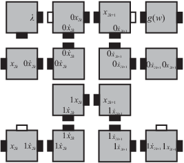
We now sketch our construction for Theorem 3.1. Figure 1 shows a very high-level overview of the main components of the construction. The general components are 1. a counter (whose base will be discussed later) which begins at a hard-coded value (also to be discussed) that counts in a zig-zag manner, with one row performing an increment and the next performing a check to see if the counter should halt, to its maximum value to form the left side of the square, 2. a set of zig-zag columns which pass a token diagonally downward and right from the top of the counter (stopping once that token reaches the bottom) to form the majority of the square, and 3. two sets of tiles which form short rows off of the bottom and right side of the square to make its dimensions exactly $N$.

In order to mimic the cooperativity which occurs in temperature $2$ self-assembly (i.e. the attachment of a tile to an assembly via two strength-$1$ bonds), we simulate individual tiles using “gadgets” which are approximately $4\times 4$ squares of tiles as pictured in Figure 2.

In order to achieve the optimal tile type complexity mentioned above, we make use of the technique introduced in [1] in which they convert a binary number $N$ into a base $b$ number, where $b$ is the power of $2$ such that $\frac{\log N}{\log\log N}\leq b=2^{k}<\frac{2\log N}{\log\log N}$ for some positive integer $k$. This ensures that the number of positions in the base-$b$ representation of $N$ is $n=\frac{\log N}{\log b}=O\left(\frac{\log N}{\log\log N}\right)$. Thus, since each gadget in our optimal square construction representing a position of that value requires a height of $4$ tiles, the number of rows of tiles necessary for an increment row–plus a check row is–$8$. Additionally, the width of the counter will be $4n$. Let $c=\lfloor\frac{N-4n}{8}\rfloor$ be the number of pairs of rows of gadgets that the counter should assemble so that the diagonal shifter tiles can form the necessary dimensions. Next, let $r=(N-4n)\mod 8$ be the remainder necessary to pad the square out to exactly $N$. Finally, let $s=b^{\lceil\log_{b}c\rceil}-c$ be the value at which the counter begins so that, by incrementing $c-1$ times, it will reach its maximum value of $b^{\lceil\log_{b}c\rceil}-1$. The value $s$ is logically encoded into the gadgets that grow from the seed to form the first row of the binary counter in our construction.

By allowing hard-coded rows of tiles of length $4n+r$ to attach to the bottom and rows of tiles of length $r$ to the right, our square construction exactly achieves the specified dimension of $N\times N$.

The tile complexity of the initial row of the counter is $O(n)=O\left(\frac{\log N}{\log\log N}\right)$. The tile complexity of a base $b$ counter is $O(b)=O\left(\frac{\log N}{\log\log N}\right)$ and since the tile complexity blowup caused by creating the gadgets is $O(1)$, the tile complexity of the entire counter is $O\left(\frac{\log N}{\log\log N}\right)$. Note that $O(1)$ tile types are required for the diagonal shifter component. Finally, the bottom and right filler rows require $O(n)=O\left(\frac{\log N}{\log\log N}\right)$ and $O(1)$ tile types, respectively. Therefore, the tile complexity of the overall construction is $O\left(\frac{\log N}{\log\log N}\right)$.

We now present a construction using a prgTAS which is slightly less optimal than the previous rgTAS construction in terms of tile type complexity in that it self-assembles an $N\times N$ square using $O(\log N)$ tile types.

In what follows, we briefly sketch our construction for Theorem 3.2. Let $n=\left\lfloor\frac{N-1}{5}\right\rfloor$, $k=\left\lceil\log n\right\rceil$, $K=5+4k$, $n_{0}=2^{k}-n+\left\lceil\frac{K}{5}\right\rceil$ and $x=N-\left(K+5\left(n-\left\lceil\frac{K}{5}\right\rceil\right)\right)$. Intuitively, $N$ is the dimension (length of one side) of the target square $S_{N}$, $n$ is the number of count/increment row pairs that we will need in our construction, $k$ is the logical width of the counter, $K$ is the actual width of the counter in our construction, $n_{0}$ is the initial value for the counter, $2^{k}-1$ is the maximum value of the counter and $x$ is the number of rows on top of the counter that we need to fill in with generic “filler” tiles. Although not necessarily surprising, it is worthy of note–and easy to show–that $x\leq 9$. In Figure 5, we show a high-level overview of the terminal assembly produced by our construction (many details are omitted).

In our construction, we emulate the zig-zag counter of Rothemund and Winfree [19]. We utilize three different binary counters in our construction, denoted as the first, second and third counter and oriented vertically, horizontally and vertically respectively. We will discuss the general behavior of our north-growing zig-zag counter and highlight any subtle differences between the two other versions of it that we use in our construction.

The binary counter consists of a seed row, which encodes some number in binary, on top of which some number of increment/copy row pairs self-assemble in a zig-zag fashion. The top of the counter is capped off with a special cap gadget.

The Seed Row. The seed row is a row of tiles that encodes the initial value of the binary counter $n_{0}$ using $k=\left\lceil\log n\right\rceil$ bits and has a horizontal extent of $K-1$. The counter starts counting at this value and stops at $2^{k}-1$. We encode the bits of $n_{0}$ via the careful placement of the negative glue (denoted as a little white square in all of our figures). The bit 0 is encoded by positioning the negative glue so that it is facing north in a dent and a 1 is encoded by positioning the negative glue so that it is facing east in a dent; see Figure 7. This bit encoding scheme is also used in count rows whereas slightly different encoding is used for copy rows. Off the bottom of the seed row, teeth of a “comb” attach in order to fill in the bottom left corner of the square. Each tooth has length $K$ and self-assembles to the south. The actual length of the seed row–and hence the actual width of our counter in this construction–is $K$.

The Copy Rows. Copy rows self-assemble on top of increment rows (including the seed row) from left to right and have horizontal extent $K$ (the actual width of the counter). Copy rows consist of a sequence of bit gadgets that utilize geometry and the careful placement of the unique negative (white) glue in order to emulate cooperations (see Figure 6). In our construction, we have a one bit gadget for every bit in the binary representation of $n_{0}$ (this information is encoded directly into the bit gadget so that it knows which bit it is, e.g., most significant, least significant, third, etc). The bit gadgets that comprise each copy row are shown in Figure 8. In our construction, if a copy row reads a string of 1 bits, i.e., $2^{m}-1$ for some $m\in\mathbb{N}$, it will terminate the counter and allow the cap gadget to attach.

The Increment Rows. Each increment row increments the value of the counter by 1. Increment rows self-assemble from right to left (compared to left to right for copy rows–hence the zig-zag nature of our counter). Similar to copy rows, increment rows consist of a sequence of (a different type of) bit gadgets that each know “which” bit they represent. The bit gadgets for increment rows are shown in Figure 9.

The value of the final increment row in our counter is $2^{k}-1$ giving the counter an actual height of $5\left(n-\left\lceil\frac{K}{5}\right\rceil\right)$ rows of tiles. The bit pattern of $2^{k}-1$ is detected by the (final) copy row, which terminates the counting. On top of the final copy row of the counter, a special cap tile gadget attaches, which is a path of tiles that fills in–and smooths out–the top of the jagged zig-zag counter. For each value of $x$ (ranging from 1 to 9), we use a different cap tile gadget. The top portion of Figure 7 shows the two types of cap gadgets that we use in our construction–one allows additional “comb teeth” (each of varying height/length depending on $x$) to attach and the other that simply caps the counter.

Completing the Square. After–and only after–the first binary counter completes, may the construction proceed. To the upper right corner of the first binary counter, a path of tiles crawls down along the right side of the first vertical counter toward the seed tile. This path of tiles detects the seed tile via the south-facing negative glue in the lower rightmost tile in each copy row. A south-facing negative glue tells this path of tiles to “keep going.” Only the black seed tile type has an east-facing negative glue, which tells the path to “stop” and build the seed row for the second (horizontal) counter. Note that we do not encode any location information into these tiles that crawl down the right side of the first counter, which means that there are $O(1)$ such tile types participating in the formation of the path.

The second binary counter (the base of the ‘U’ backbone) behaves similarly to the first counter except its top (logically, its least significant bit) is completely smooth so as to allow the seed row of the third and final (vertical) binary counter to attach. Furthermore, the cap tile gadget for the second counter places one more row of cap tiles on top of (actually, to the right of) the second counter than the cap tile gadget did for the first counter to ensure that the terminal structure is a square. The cap tile gadget for the second counter also initiates the self-assembly of the seed row for the third–and final–binary counter.

The third (and final) counter, which happens to grow in a vertical fashion, in our construction completes the ‘U’-shaped backbone of the nearly-optimal square construction. This counter behaves similar to the first counter except its right edge is completely smooth. We also use a third type of cap tile gadget to form the smooth top of the square. This third type of cap gadget allows comb teeth (whose size depends on $x$) to bind to its north side and also shoots a path of tiles off to the left and back toward the first counter.

This path of tiles is eventually blocked by the first counter, but as this path self-assembles to the left, it allows filler tiles to fill in the interior of the square (see Figure 11 for an example) and comb teeth to attach on top.

Tile Complexity. We use $O(1)$ generic filler tiles (white tile types in our figures) that either attach on top of (or to the right of) cap rows or fill in the interior of the square. There are $O(1)$ tiles that crawl down the right side of the first binary counter. The filler tiles that fill in the bottom left corner of the square must grow to length $O(K)=O(k)$ and stop for which $O(k)$ unique tile types suffice. Finally, we must encode the appropriate bit location into every bit gadget of the seed row and every copy, increment and cap tile gadget. Since there are $O(1)$ types of bit gadgets for each row and $k$ bit locations in each of the three different counters that we use, the tile complexity of our construction is dominated by $O(k)=O(\log N)$.

It is interesting to note that our nearly-optimal construction (NOC) is essentially a spanning tree, much like the “$2N-1$” construction of [19]. However, in our NOC, we are allowed to use a single negative glue type, which–in conjunction with some clever use of geometry–allows us to emulate the cooperativity of “temperature 2” self-assembly. Furthermore, the longest simple path of tiles in Rothemund and Winfree’s “$2N-1$” construction is $2N-1=O(N)$ whereas the longest simple path of tiles in our NOC is $O\left(N\log N\right)$ but our NOC ensures that the length of every simple (un-blocked) path of tiles cannot exceed $O(\log N)$ without encountering the negative glue.

The remainder of this subsection is devoted to a brief, intuitive sketch of our construction for Theorem 4.1.

Intuitively, $\mathcal{S}$ simulates $\mathcal{T}$ by logically converting each tile type $t\in T$ into a group of tile types in $S$ that self-assemble into a macro-tile. Since each macro-tile is the same size ($12$ tiles), it is easy to compute the indices $i_{-1}<i_{0}<\cdots i_{k}$ in the definition of path simulate.

As shown in Figure 12, each $t\in T$ which can be placed in a growing compact zig-zag assembly has well-defined “input” and “output” sides (for convenience, and without loss of generality, we fix the seed row as growing from left to right). The corresponding macro-tiles are also depicted in Figure 12. (Note that the particular shapes and sizes of the macro-tiles are designed so that all macro-tiles have the same number of tiles and also exactly one path of assembly, in order to correspond to the definition of path simulate.) Double strength bonds on $t$ are simply simulated with a single strength-$1$ glue in the proper position of its macro-tile since $\mathcal{S}$ is a temperature $1$ system. Strength-$1$ glues are simulated by ensuring that every time a glue simulating a strength-$1$ glue is placed, that the adjacent location - in which a tile would be placed to bind to that glue - already also has adjacent to it a singly copy of the negative strength glue. This ordering is guaranteed by the careful design of the macro-tiles and their order of growth. In this way, whenever a tile would be placed in $\mathcal{T}$ by attaching to exactly two strength-$1$ glues, in $\mathcal{S}$ a tile is placed which binds to two strength-$1$ glues and is also repelled by a single negative strength-$1$ glue, for a total binding force of strength $1$. This provides a mechanism for cooperation by ensuring that both input glues are matched.

Figure 13 gives an example of how the growth of the first few rows of $\mathcal{T}$ are simulated by the growth of connected gadgets in $\mathcal{S}$. It is clear that $\mathcal{S}$ will exactly path simulate $\mathcal{T}$ at scale factor $12$. Since $\mathcal{T}$ is an arbitrary compact zig-zag TAS and $\mathcal{S}$ is an rgTAS, Theorem 4.1 is proven.

The remainder of this subsection is devoted to a brief, intuitive sketch of our construction for Theorem 4.2.

Intuitively, $\mathcal{S}$ simulates $\mathcal{T}$ by logically converting each tile type $t\in T$ into a group (path) of tile types in $S$ that self-assemble into a macro-tile. Let $G$ be the number of unique strength-$1$ north/south glues in $T$. Each macro-tile is a path of $2\left\lceil\log G\right\rceil+30$ tiles and forms in its entirety before allowing the next macro-tile to form, whence the scale factor in our construction is $O\left(\log G\right)=O(\log|T|)$. Moreover, we can use the fact that macro-tiles are all the same size in order to easily compute the indices $i_{-1}<i_{0}<\cdots i_{k}$ in the definition of path simulate.

As shown in Figure 14a, each $t\in T$ has well-defined “input” and “output” sides (for convenience, and without loss of generality, we fix the seed row as growing from left to right), some of which may be the empty glue. The corresponding macro-tiles are depicted in Figure 14b. We encode each north/south glue in $T$ as a unique $(G+1)$-bit binary string (we also encode the empty glue label, whence each glue is represented as a $(G+1)$-bit binary string). We then encode each binary string (representing a glue) as a path of bumps and dents along the north and south side of the appropriate macro-tile(s). Into the bumps and dents, we carefully place the negative glue type to either represent a ‘0’ or a ‘1’ bit–similar to the construction for Theorem 3.2. Note that we do not represent the “east/west” or strength-$2$ “north/south” glues of $T$ in this manner because in this case we encode these glue types in $T$ on the glues of the tiles which serve as the beginning and ends (inputs and outputs) of the paths forming the corresponding macro-tiles.

A macro-tile that represents a tile type $t\in T$ that binds via two “input” sides (e.g., south-east/south-west) self-assembles in two logical stages: reading the input glues and unpacking the output glues. In what follows, we will discuss the macro-tiles that represent tiles that have south/east input sides. The macro-tiles that emulate tiles with south/west input sides are constructed similarly.

Reading the Input Glues. In the first stage of the self-assembly of a “south-east input” macro-tile, an initial portion of its path crawls (either to the left or to the right) across the top of an existing macro tile. In doing so, the growing macro-tile path “reads” in, via a series of appropriate-placements of the negative glue in bumps and dents, a binary string, which represents a glue type in $T$. The method of “reading” a bit is depicted in Figure 14c and is similar to the technique used in Theorem 3.2 (see also Figure 6).

For each $0\leq i<G+1$, we have a group of tile types that are responsible for collecting the $i^{\textmd{th}}$ bit of a binary string as they assemble a path to the left while “remembering” the previous $0\leq j<i$ bits (see Figure 16). Note that not every tile type in the group that reads the $i^{\textmd{th}}$ bit needs to remember all $G+1$ bits. In fact, it suffices for the group of tiles responsible for reading the $i^{\textmd{th}}$ bit to only remember $i$ bits. In order to do this, we use $O\left(2^{0}+2^{1}+\cdots+2^{i}\right)=O\left(2^{i+1}\right)$ unique tile types, i.e., $O(1)$ tile types for each of the $2^{j}$ $j$-bit binary strings, whence we must have a total of $O\left(2^{\log(G+1)}\right)=O(G)=O(|T|)$ unique tile types to read a glue from the top of an existing macro-tile (these tile types for a south-east input, north-west output macro-tile are shown in Figure 15). Once all $G+1$ bits have been collected, we have a group of $O(G)$ unique tile types to convert the east input glue, along with the south input glue, into the appropriate output glue(s) for the macro-tile..

Unpacking the Output Glues. After the output glue(s) of a macro-tile have been determined, the macro-tile path crawls back across itself and determines when to “stop” via the checkered tiles in Figure 14(b). Then the path crawls, once again, back across itself and “unpacks” the north output glue (it does not have to unpack the west output glue by the way we encode the east/west glue types in $T$ in macro-tiles). We accomplish this task in a manner that is similar to–but essentially the opposite of–reading in a $(G+1)$-bit binary string. To do this, we use $O\left(G\right)=O(|T|)$ unique tile types (these tile types for a south-east input, north-west output macro tile are shown in Figure 17.

Finally, a macro-tile in $S$ that represents a tile type $t\in T$ that binds via a single, strength-$2$, input(output) side does not perform any input reading or output unpacking because we encode each strength-$2$ glue in $T$ as a unique strength-$1$ glue in $S$. Thus, when such a macro tile self-assembles, it does so in a single logical stage.

References

- [1] Leonard Adleman, Qi Cheng, Ashish Goel, and Ming-Deh Huang, Running time and program size for self-assembled squares, Proceedings of the thirty-third annual ACM Symposium on Theory of Computing (New York, NY, USA), ACM, 2001, pp. 740–748.
- [2] Robert D. Barish, Rebecca Schulman, Paul W. Rothemund, and Erik Winfree, An information-bearing seed for nucleating algorithmic self-assembly, Proceedings of the National Academy of Sciences 106 (2009), no. 15, 6054–6059.
- [3] Ho-Lin Chen, Rebecca Schulman, Ashish Goel, and Erik Winfree, Reducing facet nucleation during algorithmic self-assembly, Nano Letters 7 (2007), no. 9, 2913–2919.
- [4] Matthew Cook, Yunhui Fu, and Robert Schweller, Temperature 1 self-assembly: Deterministic assembly in 3d and probabilistic assembly in 2d, Proceedings of the 22nd Annual ACM-SIAM Symposium on Discrete Algorithms, 2011.
- [5] David Doty, Randomized self-assembly for exact shapes, SIAM Journal on Computing 39 (2010), no. 8, 3521–3552.
- [6] David Doty, Lila Kari, and Benoît Masson, Negative interactions in irreversible self-assembly, Algorithmica, to appear. Preliminary version appeared in DNA 2010.
- [7] David Doty, Jack H. Lutz, Matthew J. Patitz, Scott M. Summers, and Damien Woods, Intrinsic universality in self-assembly, Proceedings of the 27th International Symposium on Theoretical Aspects of Computer Science, 2009, pp. 275–286.
- [8] David Doty, Matthew J. Patitz, Dustin Reishus, Robert T. Schweller, and Scott M. Summers, Strong fault-tolerance for self-assembly with fuzzy temperature, Proceedings of the 51st Annual IEEE Symposium on Foundations of Computer Science (FOCS 2010), 2010, pp. 417–426.
- [9] David Doty, Matthew J. Patitz, and Scott M. Summers, Limitations of self-assembly at temperature 1, Theoretical Computer Science 412 (2011), 145–158.
- [10] Ming-Yang Kao and Robert T. Schweller, Reducing tile complexity for self-assembly through temperature programming, Proceedings of the 17th Annual ACM-SIAM Symposium on Discrete Algorithms (SODA 2006), Miami, Florida, Jan. 2006, pp. 571-580, 2007.
- [11] , Randomized self-assembly for approximate shapes, International Colloqium on Automata, Languages, and Programming, Lecture Notes in Computer Science, vol. 5125, Springer, 2008, pp. 370–384.
- [12] Joseph M. Kinsella and Albena Ivanisevic, Enzymatic clipping of dna wires coated with magnetic nanoparticles, Journal of the American Chemical Society 127 (2005), no. 10, 3276–3277.
- [13] James I. Lathrop, Jack H. Lutz, and Scott M. Summers, Strict self-assembly of discrete Sierpinski triangles, Theoretical Computer Science 410 (2009), 384–405.
- [14] Urmi Majumder and John Reif, A framework for designing novel magnetic tiles capable of complex self-assemblies, Unconventional Computing (Cristian Calude, José Costa, Rudolf Freund, Marion Oswald, and Grzegorz Rozenberg, eds.), Lecture Notes in Computer Science, vol. 5204, Springer Berlin / Heidelberg, 2008, pp. 129–145.
- [15] Chengde Mao, Weiqiong Sun, and Nadrian C. Seeman, Designed two-dimensional DNA holliday junction arrays visualized by atomic force microscopy., Journal of the American Chemical Society 121 (1999), no. 23, 5437–5443.
- [16] John H. Reif, Sudheer Sahu, and Peng Yin, Complexity of graph self-assembly in accretive systems and self-destructible systems, Theor. Comput. Sci. 412 (2011), no. 17, 1592–1605.
- [17] David Rickwood and Vera Lund, Attachment of dna and oligonucleotides to magnetic particles: methods and applications, Fresenius’ Journal of Analytical Chemistry 330 (1988), 330–330, 10.1007/BF00469247.
- [18] Paul W. K. Rothemund, Theory and experiments in algorithmic self-assembly, Ph.D. thesis, University of Southern California, December 2001.
- [19] Paul W. K. Rothemund and Erik Winfree, The program-size complexity of self-assembled squares (extended abstract), STOC ’00: Proceedings of the thirty-second annual ACM Symposium on Theory of Computing (Portland, Oregon, United States), ACM, 2000, pp. 459–468.
- [20] Paul W.K. Rothemund, Nick Papadakis, and Erik Winfree, Algorithmic self-assembly of DNA Sierpinski triangles, PLoS Biology 2 (2004), no. 12, 2041–2053.
- [21] David Soloveichik and Erik Winfree, Complexity of self-assembled shapes, SIAM Journal on Computing 36 (2007), no. 6, 1544–1569.
- [22] Erik Winfree, Algorithmic self-assembly of DNA, Ph.D. thesis, California Institute of Technology, June 1998.
- [23] Erik Winfree, Furong Liu, Lisa A. Wenzler, and Nadrian C. Seeman, Design and self-assembly of two-dimensional DNA crystals., Nature 394 (1998), no. 6693, 539–44.