Study of noise effects in electrical impedance tomography with resistor networks

We denote by ${\bf F}:C(\Omega)\to\mathbb{R}^{g}$, the forward map that associates to a conductivity $\sigma$ the vector of measurements ${\bf F}(\sigma)$ of the DtN map. The measurement operation is explained in detail in section 3.1.1. It amounts to recording voltages and currents at $n$ electrodes on the boundary. The dimension $g=n(n-1)/2$ of the data vector ${\bf d}$ corresponds to the number of independent measurements that can be made with $n$ electrodes. The data model is

with ${\bm{\epsilon}}$ the noise vector. The notation ${\mathcal{N}}\left({\bf 0},\mathcal{C}\right)$ states that ${\bm{\epsilon}}$ is Gaussian (multivariate normal), with mean zero and diagonal covariance $\mathcal{C}$. We refer to section 3.1.1 for an explanation of the uncorrelation of the components of ${\bm{\epsilon}}$.

We parametrize the conductivity as in (1) with a vector ${\bf s}\in\mathbb{R}^{g}$, with $g=n(n-1)/2$ being the same dimension as the data space. Since the data ${\bf d}$ is tainted with noise, we treat ${\bf s}$ as a continuum random variable, and denote by ${\bm{\pi}}_{{}_{\mathrm{pr}}}({\bf s})$ its prior probability density. The likelihood function ${\bm{\pi}}({\bf d}|{\bf s})$ is the probability density of ${\bf d}$ conditioned to knowing ${\bf s}$. Given our Gaussian noise model, it takes the form

where $|\mathcal{C}|$ is the determinant of the covariance $\mathcal{C}$. The estimation of ${\bf s}$ is based on the conditional (posterior) density ${\bm{\pi}}({\bf s}|{\bf d})$. It is defined by Bayes’ rule [35, 22]

where ${\bm{\pi}}({\bf s},{\bf d})$ is the joint probability density of $({\bf s},{\bf d})$. The marginal

is just a normalization that plays no role in the estimation. The prior density ${\bm{\pi}}_{{}_{\mathrm{pr}}}({\bf s})$ may introduce a regularization in the inverse problem [29, Chapter 3]. The priors used in our study are summarized in A. They all ensure that the reconstructions $\sigma({\bf x})$ are positive.

We consider maximum a posteriori (MAP) estimates of the conductivity

which maximize the conditional probability density $\pi({\bf s}|{\bf d})$. The vector ${\bf s}_{{}_{\mathrm{MAP}}}$ of parameters solves the optimization problem

The MAP estimates ${\bf s}_{{}_{\mathrm{MAP}}}$ are random, because they depend on the noise ${\bm{\epsilon}}$ in the measurements. To quantify their uncertainty, we approximate their variance using a large number $M$ of independent samples ${\bf s}_{{}_{\mathrm{MAP}}}^{(m)}$, determined from (7) and data (2) with draws ${\bm{\epsilon}}^{(m)}\in\mathcal{N}\left({\bf 0},\mathcal{C}\right)$ of the noise,

Then, we compare $\mbox{Var}[{\bf s}]$ to the optimal variance, which is the right hand side in the Cramér-Rao bound [35, Corollary 5.23],

The notation $\mathbb{E}_{{\bf s}_{\star}}$ indicates that the mean (expectation) depends on the true vector of parameters ${\bf s}_{\star}$. The bias factor ${\bf b}({\bf s})$ is defined by

where $\nabla$ denotes gradient with respect to ${\bf s}$, and ${\mathcal{I}}({\bf s})$ is the Fischer information matrix [35, Section 2.3]. It measures how much information the data ${\bf d}$ carry about the parameter ${\bf s}_{\star}$. The Fisher matrix is in $\mathbb{R}^{g\times g}$, with entries

Since the likelihood $\pi({\bf d}|{\bf s})$ is Gaussian, we obtain under the natural assumption that the noise covariance $\mathcal{C}$ is independent of ${\bf s}$, that

where $D_{\bf s}\mathcal{S}({\bf s})$ is the Jacobian of $\mathcal{S}({\bf s})$ evaluated at ${\bf s}$ and $D_{\sigma}{\bf F}(\sigma)$ is the Jacobian of ${\bf F}(\sigma)$ evaluated at $\sigma$. We take as the true ${\bf s}_{\star}$ the solution of the optimization problem (7), with noiseless data and upper/lower bound prior (22). The bias ${\bf b}({\bf s}_{\star})$ is approximated via Monte Carlo simulations, from a large sample of draws. The bound (9) is evaluated and displayed in section 5.2.

We consider three different parametrizations:

• •

  piecewise linear on uniform grid: The entries in ${\bf s}$ are pointwise values of $\sigma({\bf x})$ on a uniform tensor product grid. The conductivity is piecewise linear on a Delaunay triangulation of the grid points.

• •

  piecewise linear on optimal grid: The conductivity and the parameters are defined as above, but with grid points from the so-called “optimal grid” (see section 3.2.1).

• •

  resistor network: The parameters ${\bf s}$ are (up to known multiplicative constants) the conductors in a network that has the same electrical response (DtN map) as the electrical response at the electrodes of the unknown conductivity. This parametrization is discussed in more detail in section 2.3.

In the first two parametrizations the conductivity depends linearly on ${\bf s}$. It is the piecewise linear interpolation of the entries in ${\bf s}$, between grid nodes ${\bf x}_{1},\ldots,{\bf x}_{g}$,

Here $\phi_{i}$ are piecewise linear basis functions on a Delaunay triangulation of the nodes ${\bf x}_{i}$, satisfying the usual property $\phi_{i}({\bf x}_{j})=\delta_{ij}$, with the Kronecker delta notation.

In the resistor network parametrization the conductivity depends nonlinearly on the parameters ${\bf s}$. The dependence is given in equation (16), in terms of the resistor network reduced model of (1). We emphasize that the resistor network parametrization cannot be written in the form (13). One way of comparing it to the linear case (13) is to consider a small perturbation $\delta{\bf s}\equiv(\delta s_{1},\ldots,\delta s_{g})^{T}$ of some reference $\overline{{\bf s}}$, and linearize

Here the $\phi_{i}$ are the “columns” of the Jacobian $D_{\bf s}\mathcal{S}(\overline{{\bf s}})$ of the parametrization operator $\mathcal{S}$ with respect to ${\bf s}$, and evaluated at $\overline{{\bf s}}$. We call these $\phi_{i}$ sensitivity basis functions.

For a given resistor network with $n$ boundary nodes and $g=n(n-1)/2$ resistors (one per edge), we denote by $\mathbb{F}:\mathbb{R}^{g}_{+}\to\mathbb{R}^{g}$ the discrete forward map which maps the vector of positive conductances of the network to a vector of $g$ independent entries of the Dirichlet-to-Neumann map of the network. The choice and ordering of the independent entries is identical to that of ${\bf F}$ in section 2.1. We assume that the topology (underlying graph) of the network is such that $\mathbb{F}$ admits a left inverse $\mathbb{F}^{-1}$, i.e. $\mathbb{F}^{-1}(\mathbb{F}({\bm{\gamma}}))={\bm{\gamma}}$ for all ${\bm{\gamma}}>0$. Such topologies are given in section 3.1.2.

In the resistor network parametrization we let

Here the $\gamma_{i}$ are the conductances of the network that has the same electrical response as that measured for $\sigma$, i.e. ${\bf F}(\sigma)=\mathbb{F}({\bm{\gamma}})$, for ${\bm{\gamma}}=(\gamma_{1},\ldots,\gamma_{g})^{T}$. Similarly, ${\bm{\gamma}}^{(1)}=(\gamma_{1}^{(1)},\ldots,\gamma_{g}^{(1)})^{T}$ satisfies ${\bf F}(1)=\mathbb{F}({\bm{\gamma}}^{(1)})$. Hence, it is easy to compute ${\bf s}$ from knowledge of $\sigma$ and $\mathbb{F}^{-1}$.

The mapping $\mathcal{S}$ in the resistor network parametrization is defined implicitly by

where the product of the vectors ${\bf s}$ and ${\bm{\gamma}}^{(1)}$ is understood componentwise. There are many functions that satisfy (15). We define $\mathcal{S}({\bf s})$ for the resistor network parametrization as the limit of the Gauss-Newton sequence $\{\kappa_{j}\}_{{}_{j\geq 0}}$ defined in (15),

The starting point in the Gauss-Newton iteration is $\kappa_{o}({\bf x})=\ln(\sigma^{o}({\bf x}))$, where $\sigma^{o}({\bf x})$ is the piecewise linear interpolation of the discrete values ${\bf s}$ on the optimal grid defined in section 3.2.1. In practice, the evaluation of (16) is computationally efficient because iteration (15) converges quickly, basically after one step, as shown in [9, 23].

Recall that for the resistor network parametrization, the mapping $\mathcal{S}$ is non-linear and thus cannot be written as an expansion in basis of functions, as in (13). To compare it to parametrizations of the form (13), we look at its linearization around reference parameters $\overline{{\bf s}}$ to obtain (14). The basis functions $\phi_{k}$ are then the “columns” of $D_{\bf s}\mathcal{S}(\overline{{\bf s}})$, which can be determined by differentiating (15) with respect to ${\bf s}$,

The sensitivity functions $D_{\sigma}{\bm{\gamma}}({\bf x})$ are defined in section 3.2.1 and are evaluated at $\overline{\sigma}=\mathcal{S}(\overline{{\bf s}})$. They give the sensitivity of the resistors ${\bm{\gamma}}$ to changes in the conductivity, and are an important ingredient of the inversion algorithm that is reviewed in section 3.

The linearized problem is studied in section 5.1. In this case it it is known [35, Section 5.1] that the Cramér-Rao bound is attained by the variance of the MAP estimates. The variance depends of course on the parametrization (1) used in the estimation. The results say that when we take piecewise linear interpolations of the parameters ${\bf s}$ on the equidistant or the optimal grids, we obtain much larger variances than if we use the sensitivity basis functions. That is to say, the sensitivity basis functions lead to better estimates than the piecewise linear ones, even when we interpolate on the optimal grids. We also show in section 5.2 that the nonlinear estimation based on resistor networks is efficient, in the sense that the sample variance is very close to the Cramér-Rao bound.

Resistor networks arise naturally in finite volume discretizations of equation (1) on staggered grids with interlacing primary and dual grid lines that may be curvilinear. The potential is discretized at the primary nodes $P_{i,j}$, the intersections of the primary grid lines, $u_{i,j}\approx u(P_{i,j}).$ Each node $P_{i,j}\in\Omega$ is surrounded by a dual cell $C_{i,j}$, as shown in Figure 1. Integrating (1) over the cells $C_{i,j}$, using the divergence theorem, and approximating the boundary fluxes with finite differences we obtain a system of linear equations of the form

Equations (1) are Kirchhoff’s node law for the interior nodes of the resistor network with graph $\Gamma=(\mathcal{P},\mathcal{E})$. Here $\mathcal{P}=\{P_{i,j}\}$ is the set of primary nodes, given by the union of the disjoint sets $\mathcal{P}_{{}_{\mathcal{B}}}$ and $\mathcal{P}_{{}_{\mathcal{I}}}$ of boundary and interior nodes. Adjacent primary nodes are connected by edges, the elements of the set $\mathcal{E}\subset\mathcal{P}\times\mathcal{P}$. The network is the pair $(\Gamma,{\bm{\gamma}})$, with ${\bm{\gamma}}\in\mathbb{R}_{+}^{|\mathcal{E}|}$ the vector with entries given by the conductances (inverse of resistances) $\gamma_{\alpha,\beta}>0$ of the edges, following a preassigned ordering of $\mathcal{E}$. Here $(\alpha,\beta)\in\left\{\left(i,j\pm\frac{1}{2}\right),\;\left(i\pm\frac{1}{2},j\right)\right\}$.

We relate the conductances $\gamma_{\alpha,\beta}$ and $\sigma$ by

where $L$ denotes the arclengths of the primary edges $E_{\alpha,\beta}$ and dual edges $\Sigma_{\alpha,\beta}$. The points $P_{\alpha,\beta}$ are located at the intersections of the primary and dual grid segments $E_{\alpha,\beta}$ and $\Sigma_{\alpha,\beta}$.

The forward problem for a known network $(\Gamma,{\bm{\gamma}})$ amounts to determining the potential function $\mathcal{U}:\mathcal{P}\to\mathbb{R}$, with $u_{i,j}=\mathcal{U}(P_{i,j})$ satisfying the conservation of currents (1) at the interior nodes, and Dirichlet boundary conditions

We denote the number of boundary nodes by $n$. The entries in the vector $u_{{}_{\mathcal{B}}}\in\mathbb{R}^{n}$ may be related to the continuum boundary potential $V$ as explained below, in section 3.1.1.

The inverse problem for the network seeks the conductances ${\bm{\gamma}}$ from the discrete DtN map $\Lambda_{\bm{\gamma}}$. The graph $\Gamma$ is known, and the DtN map is a matrix in $\mathbb{R}^{n\times n}$ that maps the vector $u_{{}_{\mathcal{B}}}$ of boundary potentials to the vector $J_{{}_{\mathcal{B}}}$ of boundary current fluxes. Since we consider the two dimensional problem, all the graphs $\Gamma$ are circular planar graphs [15, 16], i.e. graphs that can be embedded in the plane with no crossing edges and with all boundary nodes $\mathcal{P}_{\mathcal{B}}$ lying on a circle.

We denote by $\sigma_{\star}$ the true conductivity, to distinguish it from the estimates that we denote generically by $\sigma$. The relations (2) between ${\bm{\gamma}}$ and $\sigma_{\star}$ have been derived in the discretization of the forward problem. We use them for the conductances of the network $(\Gamma,{\bm{\gamma}})$ recovered from the measurements ${\bf F}(\sigma_{\star})$, in order to estimate $\sigma_{\star}$. This does not work unless we use a special grid in (2) [9, 11]. The idea behind the inversion on optimal grids is that the geometrical factors $L(\Sigma_{\alpha,\beta})/L(E_{\alpha,\beta})$ and the distribution of the points $P_{\alpha,\beta}$ in (2) depend weakly on $\sigma$. Therefore, we can determine both the geometrical factors and the grid nodes from the resistor network $(\Gamma,{\bm{\gamma}}^{(1)})$, with the same graph $\Gamma$ as before, and $\mathbb{F}({\bm{\gamma}}^{(1)})={\bf F}(1).$ These are the measurements of the DtN map for constant conductivity $\sigma\equiv 1$, that we can compute, and $\gamma^{(1)}_{\alpha,\beta}\approx{L(\Sigma_{\alpha,\beta})}/{L(E_{\alpha,\beta})}.$ We obtain the pointwise estimates

that we place in $\Omega$ at points $P_{\alpha,\beta}$ determined from a sensitivity analysis of the DtN map, as we explain next.

We solve equation (1), with a second order finite volume method on a very fine, uniform, tensor product grid, with $N\gg n$ nodes on the boundary. This approximates $\mathcal{M}_{N}(\Lambda_{\sigma_{\star}})$, where $\mathcal{M}_{N}$ is the measurement operator of section 3.1.1. The noise ${\bm{\epsilon}}$ in (2) is given by

We use two noise models, defined in terms of the noise level $\ell$ and a symmetric $N\times N$ matrix ${\bm{\eta}}$, with Gaussian, identically distributed entries with mean zero and variance one. The entries in ${\bm{\eta}}$ on and above the diagonal are uncorrelated. The first model scales the noise by the entries of the DtN map for constant conductivity $\sigma\equiv 1$,

where symbol $\cdot$ stands for componentwise multiplication. The scaling makes the noise easier to deal with, and the model is somewhat similar to multiplicative noise. The second noise model is

where $\|~\|$ is a matrix norm that approximates the continuum $H^{1/2}(\mathcal{B})\to H^{-1/2}(\mathcal{B})$ operator norm. It is defined in C.

The direct, layer peeling algorithms described in [15, 13, 10] are fast, but highly unstable and can be used only for very small noise. It is not known how to regularize layer peeling algorithms. To deal with the instability, we can only reduce the size of the network, as was done in [9]. However, simply reducing the network size is not sufficient for the larger noise levels considered in the simulations. We use instead the more robust Gauss-Newton method described below, which allows regularization. The Gauss-Newton method is more expensive than layer peeling (about 20 times more expensive for $n=7$), but the computational cost is reasonable because the dimension $g$ of the vector of unknown conductances is small for noisy data, and the Jacobian is relatively inexpensive to compute.

The Gauss-Newton method determines the log-conductances ${\bm{\kappa}}=\ln({\bm{\gamma}})$ in the network $(\Gamma,{\bm{\gamma}})$ (with topology $\Gamma$ fixed) by minimizing the objective functional

over ${\bm{\kappa}}\in\mathbb{R}^{g}$. Thus, the positivity of the conductances ${\bm{\gamma}}=\exp({\bm{\kappa}})$ is satisfied automatically. The first term in (19) measures the misfit between the measured data ${\bf d}$ modeled by (2), and the data produced by a network with log-conductances ${\bm{\kappa}}$. Here $\mathcal{C}$ is the covariance matrix of the measurements. The second term in (19) is a Tikhonov type regularization penalizing the distance from some reference log-conductances ${\bm{\kappa}}_{\mathrm{ref}}$. The parameter $\alpha>0$ determines the strength of the penalty term.

In our numerical experiments, the Gauss-Newton approximation of the Hessian of $\mathcal{O}({\bm{\kappa}})$ is further regularized by adding $10^{-4}/\mathcal{C}_{1,1}$ to its diagonal. The iterations are stopped either when the norm of the gradient of $\mathcal{O}({\bm{\kappa}})$ is $10^{-4}$ smaller than that at the initial iterate, or when the maximum number of iterations (300) is reached. The initial iterate is ${\bm{\kappa}}=\ln({\bm{\gamma}}^{(1)})$, and we take as reference log-conductances ${\bm{\kappa}}_{\mathrm{ref}}=\ln({\bm{\gamma}}^{(1)})$.

We show in Figures 3 and 4 the reconstructions of the true smooth and piecewise constant conductivities displayed in Figure 2. The reconstructions are obtained in the full and partial boundary setups, and for noiseless data. Two distinct cases of partial boundary measurements are considered. In the one-sided case the accessible boundary $\mathcal{B}_{A}$ consists of a single connected segment of $\mathcal{B}$. In the two-sided case the accessible boundary $\mathcal{B}_{A}$ consists of two disjoint segments of $\mathcal{B}$.

We display in the top row of Figures 3 and 4 the initial guess $\sigma^{o}({\bf x})$ of the Gauss-Newton iteration (15). It is the piecewise linear interpolation of the values $\sigma^{o}(P_{\alpha,\beta})=\sigma_{k(\alpha,\beta)}$, where $\sigma_{k}$ are obtained from (8), and the optimal grid nodes $P_{\alpha,\beta}$ are defined by (10). The function $\sigma^{o}({\bf x})$ is linear on the triangles obtained by a Delaunay triangulation of the points $P_{\alpha,\beta}$. In the partial boundary measurements case we display $\sigma^{o}({\bf x})$ in the subdomain delimited by the accessible boundary and the segmented arc connecting the innermost grid points. We set $\sigma^{o}({\bf x})$ to the constant value one in the remainder of the domain. The plots in the bottom row in Figures 3 and 4 display the result of one step of the Gauss-Newton iteration described in section 3.2.2.

The network topologies are defined in B. The reconstructions from full boundary data are in the left column in Figures 3 and 4. They are obtained with a circular network $C\left(\frac{n-1}{2},n\right)$, with $n=29$. The reconstructions with the one-sided partial boundary measurements are in the middle column, and they are obtained with a pyramidal resistor network $\Gamma_{n}$, for $n=16$. The reconstructions with the two-sided boundary measurements are in the right column. They are obtained with a resistor network $T_{n}$, for $n=16$.

The results in this section are for linearization at the constant conductivity $\overline{\sigma}({\bf x})\equiv 1$, with additive noise modeled as in (18). All the three parametrizations described in section 2.2 represent exactly $\overline{\sigma}\equiv 1$, with a parameter vector ${\bf s}$ of all ones, i.e. $\mathcal{S}(\bm{1})=1$. Hence, the linearization of the forward map around $\overline{{\bf s}}=1$ can be written as

for a small perturbation $\delta{\bf s}$ of the parameters. If we discretize the conductivity on a fine grid with $N_{\sigma}$ points, the Jacobian $D_{\sigma}{\bf F}(1)$ is a $g\times N_{\sigma}$ matrix, and the Jacobian $D_{\bf s}\mathcal{S}(\bm{1})$ is an $N_{\sigma}\times g$ matrix with columns given by the basis functions $\phi_{k}$ in (14).

The estimate $\sigma_{{}_{\mathrm{MAP}}}$ is calculated by solving the optimization problem (7), with the linearization (20) of the forward map, and the upper/lower bound prior (22). This optimization is a quadratic programming problem that we solve using the software QPC [37]. The mean and variance of $\sigma_{{}_{\mathrm{MAP}}}$ are estimated with Monte Carlo simulations

using $M=1000$ samples. We do not show the mean $\left<\sigma({\bf x})\right>$ because it is basically $\overline{\sigma}({\bf x})$ for all the cases that we present below. The standard deviation $\left\{\mbox{Var}[\sigma({\bf x})]\right\}^{1/2}$ is shown in Figure 5 for the case of full boundary measurements, and the three parametrizations described in section 2.2. The noise level is $\ell=0.01\%$. We choose it so small to minimize the action of the positivity constraints imposed by the prior. Larger noise levels are considered later in the paper.

With the resistor network parametrization, the standard deviation is smaller and does not increase toward the center of the domain. Also there are no active positivity constraints. The random fluctuations of $\sigma_{{}_{\mathrm{MAP}}}$ in Figure 5 (b) lie mostly within three standard deviations, and are much smaller than the background conductivity $\overline{\sigma}\equiv 1$.

The piecewise linear parametrization on the equidistant grid gives a large, order one standard deviation in the center of the domain. The positivity constraints are active in $81.6\%$ of realizations. Surprisingly, the piecewise linear parametrization on the optimal grid is worse. Its standard deviation is large, of order one in most of the domain, and the positivity constraints are active in $61.1\%$ realizations. This shows that it is not enough to distribute the parameters on the optimal grid.

The same conclusion can be reached from Figure 6, where we display the condition number of the matrix $D_{\sigma}{\bf F}(1)D_{\bf s}\mathcal{S}(\bm{1})$, as a function of the number $n$ of boundary points. The condition number increases exponentially with $n$, as expected from the exponential ill-posedness of the problem. However, the rate of increase is smaller for the resistor network parametrization.

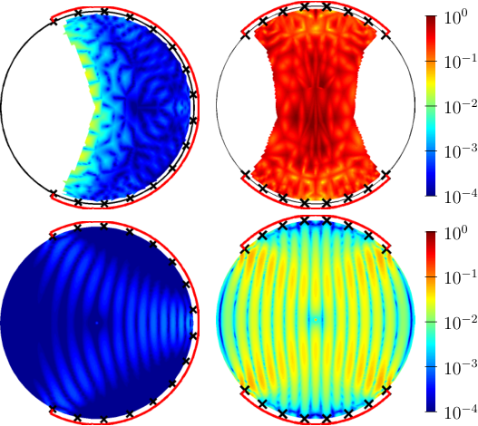
The standard deviation $\left\{\mbox{Var}[\sigma({\bf x})]\right\}^{1/2}$ is shown in Figure 7 for the case of one and two-sided boundary measurements. We use a much smaller noise level ($\ell=10^{-8}\%$, additive model (18)) in the partial measurements case than in the full data case, because we compute the standard deviation for bigger networks ($n=16$, same network size as in the reconstructions of Figures 3 and 4). Since the condition number of the linearized problem grows exponentially as we increase $n$, only very small levels of noise can be used for $n=16$. We present the results for the piecewise linear parametrization on the optimal grid (top row) and the resistor network parametrization (bottom row).

We reach the same conclusion as before. The resistor network parametrization gives a smaller standard deviation, that does not increase toward the inaccessible region. The piecewise linear parametrization on the optimal grid gives a large standard deviation near the inaccessible region in the one-sided case, and in the whole domain in the two-sided case. The positivity constraints are active in most realizations for the piecewise linear parametrization. They are not active for the resistor network parametrization.

We study the statistics (mean and standard deviation) of the MAP estimates of the parameters ${\bf s}_{{}_{\mathrm{MAP}}}$ and the conductivities $\sigma_{{}_{\mathrm{MAP}}}=\mathcal{S}({\bf s}_{{}_{\mathrm{MAP}}})$, which come from minimizing the functional (7). The study can be done for both the full and partial boundary measurement setup, but we present here only the full measurements case. We consider first, in section 5.2.1, very small noise so that we can use the fast layer peeling inversion algorithm to find the minimizer of (7), with resistor network parametrization and upper/lower bound prior (22). The speed of the algorithm allows us to compute the Cramér-Rao lower bound in a reasonable amount of time. We do not calculate the bound for larger noise, where we use regularized Gauss-Newton to determine the resistors, because of the computational cost. However, we do show in section 5.2.2 the bias and relative standard deviation of the reconstructions, and we also compare in section 5.2.3 the results to those with a piecewise linear discretization and Gaussian prior on the conductivity (23).

References

- [1] G. Alessandrini. Stable determination of conductivity by boundary measurements. Applicable Analysis, 27(1):153–172, 1988.
- [2] G. Alessandrini and S. Vessella. Lipschitz stability for the inverse conductivity problem. Advances in Applied Mathematics, 35(2):207–241, 2005.
- [3] H.B. Ameur, G. Chavent, and J. Jaffré. Refinement and coarsening indicators for adaptive parametrization: application to the estimation of hydraulic transmissivities. Inverse Problems, 18:775, 2002.
- [4] H.B. Ameur and B. Kaltenbacher. Regularization of parameter estimation by adaptive discretization using refinement and coarsening indicators. Journal of Inverse and Ill Posed Problems, 10(6):561–584, 2002.
- [5] K. Astala, L. Päivärinta, and M. Lassas. Calderón’s Inverse Problem for Anisotropic Conductivity in the Plane. Communications in Partial Differential Equations, 30(1):207–224, 2005.
- [6] S. Asvadurov, V. Druskin, and L. Knizhnerman. Application of the difference Gaussian rules to solution of hyperbolic problems. Journal of Computational Physics, 158(1):116–135, 2000.
- [7] J.A. Barcelo, T. Barcelo, and A. Ruiz. Stability of the inverse conductivity problem in the plane for less regular conductivities. Journal of Differential Equations, 173(2):231–270, 2001.
- [8] L. Borcea and V. Druskin. Optimal finite difference grids for direct and inverse Sturm-Liouville problems. Inverse Problems, 18(4):979–1002, 2002.
- [9] L. Borcea, V. Druskin, and F. Guevara Vasquez. Electrical impedance tomography with resistor networks. Inverse Problems, 24(3):035013 (31pp), 2008.
- [10] L. Borcea, V. Druskin, F. Guevara Vasquez, and A.V. Mamonov. Resistor network approaches to electrical impedance tomography. Inside Out, Mathematical Sciences Research Institute Publications, 2011.
- [11] L. Borcea, V. Druskin, and L. Knizhnerman. On the Continuum Limit of a Discrete Inverse Spectral Problem on Optimal Finite Difference Grids. Communications on Pure and Applied Mathematics, 58(9):1231, 2005.
- [12] L. Borcea, V. Druskin, and A.V. Mamonov. Circular resistor networks for electrical impedance tomography with partial boundary measurements. Inverse Problems, 26(4):045010, 2010.
- [13] L. Borcea, V. Druskin, A.V. Mamonov, and F. Guevara Vasquez. Pyramidal resistor networks for electrical impedance tomography with partial boundary measurements. Inverse Problems, 26(10):105009, 2010.
- [14] R.M. Brown and G. Uhlmann. Uniqueness in the inverse conductivity problem for nonsmooth conductivities in two dimensions . Commun. Partial Diff. Eqns, 22:1009–27, 1997.
- [15] E. Curtis, E. Mooers, and J.A. Morrow. Finding the conductors in circular networks from boundary measurements. RAIRO - Mathematical Modelling and Numerical Analysis, 28:781–814, 1994.
- [16] E.B. Curtis, D. Ingerman, and J.A. Morrow. Circular planar graphs and resistor networks. Linear Algebra and its Applications, 23:115–150, 1998.
- [17] E.B. Curtis and J.A. Morrow. Inverse problems for electrical networks. World Scientific, 2000.
- [18] Y.C. de Verdière. Reseaux electriques planaires I. Commentarii Mathematici Helvetici, 69(1):351–374, 1994.
- [19] Y.C. de Verdière, I. Gitler, and D. Vertigan. Reseaux electriques planaires II. Commentarii Mathematici Helvetici, 71(1):144–167, 1996.
- [20] V. Druskin and L. Knizhnerman. Gaussian spectral rules for second order finite-difference schemes. Numerical Algorithms, 25(1):139–159, 2000.
- [21] V. Druskin and L. Knizhnerman. Gaussian spectral rules for the three-point second differences: I. A two-point positive definite problem in a semi-infinite domain. SIAM Journal on Numerical Analysis, 37(2):403–422, 2000.
- [22] B.G. Fitzpatrick. Bayesian analysis in inverse problems. Inverse problems, 7:675, 1991.
- [23] F. Guevara Vasquez. On the Parametrization of Ill-posed Inverse Problems Arising from Elliptic Partial Differential Equations. PhD thesis, Rice University, Houston, TX, USA, 2006.
- [24] O.Y. Imanuvilov, G. Uhlmann, and M. Yamamoto. Global uniqueness from partial Cauchy data in two dimensions. Arxiv preprint arXiv:0810.2286, 2008.
- [25] D. Ingerman. Discrete and continuous Dirichlet-to-Neumann maps in the layered case. SIAM Journal on Mathematical Analysis, 31:1214–1234, 2000.
- [26] D. Ingerman, V. Druskin, and L. Knizhnerman. Optimal finite difference grids and rational approximations of the square root I. Elliptic problems. Communications on Pure and Applied Mathematics, 53(8):1039–1066, 2000.
- [27] D. Ingerman and J. A. Morrow. On a characterization of the kernel of the Dirichlet-to-Neumann map for a planar region. SIAM Journal on Applied Mathematics, 29:106–115, 1998.
- [28] D. Isaacson. Distinguishability of conductivities by electric current computed tomography. IEEE transactions on medical imaging, 5(2):91–95, 1986.
- [29] J.P. Kaipio and E. Somersalo. Statistical and computational inverse problems. Springer Science+ Business Media, Inc., 2005.
- [30] K. Knudsen, M. Lassas, J.L. Mueller, and S. Siltanen. Regularized d-bar method for the inverse conductivity problem. Inverse Problems and Imaging, 3:599–624, 2009.
- [31] H.R. MacMillan, T.A. Manteuffel, and S.F. McCormick. First-order system least squares and electrical impedance tomography. SIAM Journal on Numerical Analysis, 42(2):461–483, 2004.
- [32] A.V. Mamonov. Resistor Networks and Optimal Grids for the Numerical Solution of Electrical Impedance Tomography with Partial Boundary Measurements. PhD thesis, Rice University, Houston, TX, USA, 2010.
- [33] N. Mandache. Exponential instability in an inverse problem for the Schrodinger equation. Inverse Problems, 17(5):1435–1444, 2001.
- [34] A.I. Nachman. Global uniqueness for a two-dimensional inverse boundary value problem. Annals of Mathematics, pages 71–96, 1996.
- [35] M.J. Schervish. Theory of statistics. Springer, 1995.
- [36] A.D. Seagar. Probing with low frequency electric currents. PhD thesis, University of Canterbury, UK. Department of Electrical Engineering, 1983.
- [37] A.G. Wills and B. Ninness. QPC - Quadratic Programming in C. Webpage. http://sigpromu.org/quadprog/.