Double-Slit Experiments with Microwave Billiards
Abstract
Single and double-slit experiments are performed with two microwave billiards with the shapes of a rectangle and a quarter stadium, respectively. The classical dynamics of the former is regular, whereas that of the latter is chaotic. Microwaves can leave the billiards via slits in the boundary, forming interference patterns on a screen. The aim is to determine the effect of the billiard dynamics on their structure. For this the development of a method for the construction of a directed wave packet by means of an array of multiple antennas was crucial. The interference patterns show a sensitive dependence not only on the billiard dynamics but also on the initial position and direction of the wave packet.
pacs
05.45.Mt, 03.65.Yz, 03.65.TaI Introduction
At the beginning of the 19th century, Thomas Young performed for the first time an experiment that still attracts strong interest in physics: the interference of light beams passing through a double slit [1]. This experiment and its outcome have played a profound role in the development of optics and quantum mechanics and have been used since as a paradigm to unveil the wave nature of a number of physical entities, in particular single electrons [2, 3], neutrons [4], atoms [5, 6] and molecules [7].
Recently, Casati and Prosen carried out a numerical simulation of a double-slit experiment with a well directed Gaussian wave packet initially confined inside quantum billiards [8], whose classical dynamics are regular or chaotic. The time evolution of the wave packet is governed by the first-order time-dependent Schrödinger equation. The wave packets may leak out of the billiard via two slits in its sidewall. The interference patterns resulting from diffraction of the wave packet at the slit openings have been investigated. For the billiard with regular dynamics, the interference pattern is similar to the well-known result obtained from a double-slit experiment with plane waves in the Fraunhofer regime (far field region); i.e., the intensity encountered on a screen is equal to the sum of the intensities from the two corresponding single-slit experiments plus an interference term [9]. On the other hand, for the billiard with chaotic dynamics, the intensity on the screen is equal to the superposition of the diffraction maxima radiated from each of the single slits. As a consequence, the intensity pattern becomes unimodal.
The experiments described in the present work were initially motivated by these numerical studies. They were performed with flat cylindrical microwave cavities (also called microwave billiards) that have one or two openings in their side walls. Below a certain excitation frequency, only the lowest transverse magnetic modes with electric field perpendicular to the top and bottom plate of the cavity exist. Accordingly, there the related Helmholtz equation is identical with the time-independent Schrödinger equation of the quantum billiard of corresponding shape [10, 11]. An appropriate choice of the shape of the cavity allows the investigation of wave phenomena in quantum billiards with regular, chaotic, or mixed dynamics. In contrast to the quantum case, the electromagnetic wave equation governing the time evolution of the waves in microwave billiards is of second order. Still, as will be outlined below, the experiments provide insight into the dependence of the interference patterns resulting from such double-slit experiments on the classical dynamics.
The paper is organized as follows. Section II is devoted to the description of the experimental setup. Stationary wave patterns originating from the diffraction of electromagnetic waves emitted from a single antenna, which is situated inside the microwave billiard, at the openings are presented in Sec. III. In Sec. IV we investigate the temporal evolution of the diffracted waves in the exterior close to the slits. In Sec. V we present a new method developed for the construction of a directed initial wave packet with an array of emitting antennas. It is used to realize the situation considered in the numerical simulation of Ref. [8].
II Experiments
II.1 Billiards


The principle of the construction of the microwave billiards is illustrated in Fig. 1, which exemplifies a billiard of rectangular shape. They are composed of three plates, mm thick, made of copper as depicted in Fig. 1. The middle plate has a hole in the form of the shape of the billiard. This yields a microwave cavity with a height of mm. One of its sides [bottom side in Fig. 1] is composed of three modular bars of copper enabling the variation of the slits size and distance (see also Fig. 2) between the slits, respectively. Microwaves are excited inside the resonator via an antenna located at different positions (crosses). The interference pattern resulting from microwaves leaving the billiard via the slits is recorded on a “screen,” which consists of a second antenna moving in the exterior (see below). In order to investigate the relation between the dynamics of the corresponding classical billiard and the interference patterns, a regular billiard with rectangular form and a chaotic one with the shape of a desymmetrized tilted stadium, in the following simply called stadium, were used in the experiments. The three plates are screwed together and wires of solder are inserted into grooves along the contour of the billiard [not shown in Fig. 1] in order to improve the electrical contact between the plates. The rectangular microwave billiard has dimensions mm. The ratio of the side lengths is taken close to the golden ratio in order to avoid degeneracies of the eigenmodes. The stadium billiard is composed of a quarter circle and a trapezoid [12]. The radius of the quarter circle is mm, the length of the left side of the stadium is mm, and the length of the bottom side mm.
II.2 Measurements

The microwave power is coupled into and out of the setup with wire antennas. They consist of a straight thin wire of about 0.5 mm diameter that is soldered in a holder. The electromagnetic signal is generated by a vectorial network analyzer (VNA) of type PNA-L N5230A by Agilent Technologies. It is led to one antenna (port ) via a coaxial cable and fed into the cavity. This antenna penetrates partially into the cavity via a hole in the top plate. The output signal is received by another antenna (port ) in front of the slits outside the billiards. The ratio of the output power () and the input power () as well as the relative phase of both signals are measured. They yield the complex-valued scattering ()-matrix elements. The squared modulus of the scattering matrix is given as
| (1) |
A graphical representation of versus the excitation frequency is referred to as a frequency spectrum. Resonance frequencies of the cavity are obtained from the locations of its peaks i.e. resonances. Close to the resonance frequency of the th isolated resonance, the -matrix element can be expressed in good approximation [13, 14] as
| (2) |
where is the full width at half maximum of the resonance. The numerator is proportional to the product of the electric field strengths at the positions of the antennas, i.e.
| (3) |
Accordingly, the electric field distribution may be determined [11] by fixing the position of antenna , varying the position of antenna and measuring for each position of antenna , see below in Sec. III. The electric field intensity at antenna is proportional to and thus to .
Figure 2 illustrates schematically the experimental setup. Microwave power is coupled into the billiard through antenna , which penetrates mm into the cavity. In order to measure the leakage of microwave power through the slits to the exterior, the receiving antenna of mm length is moved outside of the billiard close to its edge with the slits (see grid of positions in Fig. 2) in steps of mm which is one third of the minimal considered wavelength. It is connected to the VNA via a flexible cable. The distance between the billiard edge and the lines of measuring points parallel to the edge (in the following referred to as the screen) varies between and mm.


The measurements were carried out in a so-called anechoic chamber (see Fig. 3). Pyramidal polyurethane foam structures VHP-12 NRL (from Emerson & Cuming) cover the whole surface of the chamber and ensure attenuation of the reflected microwave power by dB over the whole frequency range of the measurements [15]. Antenna is guided by a carriage attached to a positioning unit. This unit is driven by bipolar step motors and connected to a computerized numerical control (CNC) module. A PC program communicates with the VNA and with the CNC, enabling the control of the positioning unit and the simultaneous gathering of data. Antenna is aligned perpendicularly to the billiard plane to ensure that only the component of the electric field is detected. To prevent a change of the polarization of the electromagnetic field when it escapes into the three-dimensional free space, and to avoid parasitic reflections between the metallic parts of the measurement device and the billiard, all components are covered with microwave absorption material that consists of urethane foam sheets impregnated with carbon (EPP-51 material from ARC Technologies [16]). Moreover, the copper cable connected to the receiving antenna is coated with an absorptive double layer consisting of urethane foam EPP-51 and urethane flat plate EPF-11. The VNA is calibrated in order to remove the effects of the cables and the connectors on the measured spectra. These effects include reflections at connectors, attenuation in the cables and the time delay of the signal accumulated during its passage through the cables. For each position of antenna , the complex -matrix element is measured between antennas and from to GHz with a frequency step of or MHz. As a consequence the measurement of the frequency spectrum takes a few seconds for each of the positions of the receiving antenna.
Figure 4 shows a frequency spectrum for the rectangular (top) and the stadium (bottom) billiard. The emitting antenna was positioned inside the resonator symmetrically with respect to the slits at a distance mm from the lower billiard edge and the receiving antenna outside at the point , mm (see coordinate system introduced in Fig. 2). In both billiards the slit size is set to mm and the distance between the slits is mm. The spectrum shows many sharp peaks at resonance frequencies corresponding to quasibound modes. Below the cut-off frequency GHz defined by the width of the slits, which have the effect of a short waveguide (see Fig. 1) on microwaves leaving the billiard, the transmission amplitude is notably suppressed. Here, denotes the velocity of light. Note that, due to the short length of the waveguides, the cut-off frequency provides only an approximate value for the onset of the leakage of microwave power through the slits to the exterior.
III Stationary patterns of the intensity on the screen
In Fig. 5 we present the squared modulus of the measured transmission scattering matrix element at a resonance frequency indicated at the top of the respective panels as function of the position of antenna on the screen (solid lines) for the rectangular (top panel) and the stadium billiard (bottom panel). The screen is located at a distance mm from the bottom edge of the billiard. The slit size and the distance between the slits are mm and mm, respectively. The position of the emitting antenna is symmetrical with respect to the slits, i.e. . For the rectangular billiard, we observe an interference pattern with a central maximum located at and two symmetrical lateral maxima. If the emitting antenna is placed nonsymmetrically with respect to the slits, we obtain a very similar interference pattern, i.e., the measured patterns are nearly independent of the position of the emitting antenna as expected for a stationary field distribution inside the resonator. It should be noted that such interference patterns are observed only at frequencies of sharp resonances. The interference pattern for the rectangular billiard is well described by the Fraunhofer formula,
| (4) |
which is valid in the far field region if is fulfilled [9]. For the parameters of the setup presented in Fig. 5, . Here, and are the intensities radiated by each individual slit and the oscillatory term describes the interferences between the waves emitted through the slits [9]. Experimentally, and are obtained from measurements with, respectively, one of the slits closed. They are well described by , where . The curve obtained by inserting these intensities into Eq. (4) is plotted as dashed line in the upper panel of Fig. 5, showing very good agreement with the measured interference pattern. Similar results of a double-slit experiment with water surface waves instead of microwaves have been published in Ref. [17] where the motion of water waves in a tank with a shallow bottom was investigated. As in the case of microwaves the spatial propagation of the water waves is governed by the two-dimensional Helmholtz equation and is equivalent to the Schrödinger equation describing the dynamics in a quantum billiard of corresponding shape.
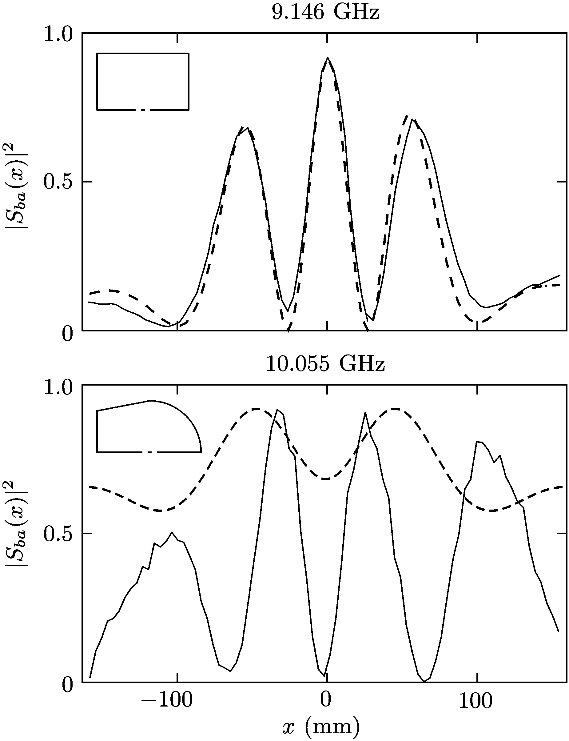

An interference pattern measured with the stadium billiard is shown as solid line in the bottom panel of Fig. 5. At we observe a maximum in the interference pattern obtained for the rectangular billiard, whereas that for the stadium billiard exhibits a minimum. According to Berry [18], the wave functions of a generic chaotic billiard can be modeled by a superposition of plane waves with the same wave number but random directions and random amplitudes , i.e.,
| (5) |
yielding a Bessel function of the first kind of order for the spatial correlator [11],
| (6) |
This implies that in the vicinity of the slits the waves are correlated as such that the interference term in Eq. (4) is modified [17]. Accordingly,
| (7) |
For wave numbers with the interference term vanishes and the intensity should be equal to the sum of the intensities of the single-slit experiments. The intensity corresponding to Eq. (7) is plotted as dashed line in the lower panel of Fig. 5. No agreement between Eq. (7) and the experimental result is found. For the example shown in Fig. 5, the visibility of the measured pattern is comparable to that for the rectangular billiard. In general the patterns exhibit only for the rectangular billiard such a clear spatial symmetry. However, for all considered cases the interference structure does not disappear, even not for wave numbers for which the interference term should vanish according to Eq. (7). It should be noted also that the results for chaotic billiards with water surface waves [17] do not provide convincing evidence that the total intensity equals the sum of the intensities for the single-slit experiments as predicted in Ref. [8].
Examples of intensity distributions in the plane close to the slits are shown in Fig. 6 for the rectangular (left panels) and stadium (right panels) billiard. The slit size is mm and the distance between the slits is set to mm. Antenna is positioned at . The grid of the positions of antenna covers an area of m2. In the upper two left panels the intensity patterns at frequencies GHz and GHz corresponding to isolated resonances are shown. They are symmetric with respect to the line , as expected due to the symmetry of the setup. In the lower left panels the intensities for frequencies chosen in the regime of overlapping resonances are shown. We observe a slightly asymmetric interference pattern. This is explicable because several modes, which are symmetric or antisymmetric with respect to the symmetry line, are excited simultaneously with different strengths such that the resulting field distribution has no spatial symmetry. Furthermore, experimental imperfections might also contribute to the observed asymmetry. For the stadium billiard (right panels of Fig. 6) the observation of non-symmetric interference patterns both for frequencies in the regimes of isolated and of overlapping resonances is attributed to the random field distribution of the corresponding modes. There are even cases where microwave power leaks out through just one slit, as, for instance, for GHz in Fig. 6. These results provide the first insight into the effect of the shape of the billiards on the interference patterns.
In order to analyze in more detail the interference patterns of the waves leaving the billiards we define the quantities
| (8) |
| (9) |
which correlate the intensities and the phases, respectively, of the electric field at points and , where denotes the central position on the screen. These correlators have been introduced and discussed in Ref. [19] and provide information about the symmetry and visibility of the interference structure. In a double-slit experiment with plane waves the phase difference of the exiting waves at the slits determines the symmetry of the obtained pattern whereas the amplitude difference should account for the visibility. If the amplitudes and the phases of the fields at the positions and coincide, i.e. if , the pattern is symmetric with visibility of .


These correlators were evaluated for the measurements shown in Fig. 6. Therefore, and the screen is located at the bottom side of the billiards at a distance from mm up to mm with a spatial resolution of mm in and . For each value of the pair was determined for values of (see Fig. 2), yielding a total number of measuring points. The parameters and are and mm, respectively. Thirty resonance frequencies of the corresponding closed billiards are chosen as excitation frequencies. Thus we obtain pairs of (, ). The resulting joint probability distribution of (, ) is shown in Fig. 7. For the rectangular billiard (left panel), the probability distribution is strongly concentrated around . This yields an evidence for the high (though not perfect) spatial symmetry of the measured interference patterns (cf. the left panels of Fig. 6). For an ideal double slit experiment with plane waves, one would expect a nonvanishing distribution only at . The distribution for the stadium billiard is shown in the right panel. It is also centered around , but in comparison to the left panel much less concentrated in the direction of the coordinate. This is expected due to the slight asymmetry in the interference patterns of the stadium billiard observed in the right panels of Fig. 6. In the top and bottom panels of Fig. 8 the distributions of, respectively, the intensity and phase correlator are presented. The distributions of are almost identical for the rectangular (solid line) and the stadium (dashed line) billiard and decay exponentially with , i.e., the visibility of the measured interference patterns is similar for both billiards (cf. Fig. 5). In contrast, the distributions of (bottom panel) differ markedly. While the distribution is peaked at for the rectangular billiard, i.e., there most patterns are symmetric, it is bell shaped and much broader around for the stadium billiard. As above, this is attributed to the strongly nonsymmetrical patterns caused by the random field distributions as shown in the right panels of Fig. 6. In conclusion, the distributions of the correlators show a clear difference for the interference patterns of the regular rectangular and the chaotic stadium billiard.
IV Temporal evolution of the fields outside the billiards
In this section we analyze and discuss the time evolution of the field in the vicinity of the double slit. The emitting antenna is placed inside the billiard symmetrically with respect to the slits at a distance of mm to the edge with the slits whereas the distance of the screen to this edge equals mm. Close to an isolated resonance, is essentially given by a modified Green function up to a factor that varies slowly with the frequency [20]. Consequently, the propagator is related to the Fourier transform of the experimentally obtained scattering matrix [21], i.e.,
| (10) |
The experimental spectra are measured at discrete frequencies in the range from to and, correspondingly, the discrete Fourier transform is evaluated in Eq. (10). The maximal time accessible is determined by , where is the frequency step used in the experiment. In the present measurements MHz, which corresponds to a maximal time of ns.
The upper panels of Fig. 9 show the time evolution of the intensity on the screen for the rectangular (left) and the stadium (right) billiard, i.e., versus the position of antenna . The time a wave emitted from antenna needs to reach antenna on the screen is called escape time. At each escape time, an interference pattern is observed as an intensity variation along . It results from the interference between the waves emitted from the two slits. As a result of the spatial symmetry of the rectangular billiard and the choice of the position of the emitting antenna at , every part of the cylindrical wave pulse emitted by this antenna with initial momentum direction travels the same path as its counterpart with . This is a consequence of the omnidirectionality of the initial wave pulse. Accordingly, these waves hit the slits with no phase difference. The positions of the maxima and minima observed in the intensity pattern in the upper left panel of Fig. 9 do not change with time. For the stadium billiard, however, there is no spatial symmetry and, consequently, the positions of the maxima and minima in the upper right part of Fig. 9 change with time.
In order to quantify how the interference patterns are influenced by the time evolution of the waves emitted from the two slits, for each position of antenna the intensities determined at discrete times are averaged over time up to ns, yielding . It should be noted that this quantity corresponds to the averaged current evaluated in the numerical simulation by Casati and Prosen [8]. The time average is performed up to ns since is negligibly small for longer times. The resulting time-averaged intensities are shown in the lower panels of Fig. 9 as solid lines. For the rectangular billiard the interference structure is still clearly visible, whereas it disappears for the stadium billiard. In addition, the sum of the time-averaged intensities obtained from two single-slit experiments in which the left, respectively, right slit was closed (dashed lines) is shown for comparison. It has no interference structure and shows a qualitative agreement with the time-averaged intensity resulting from the double-slit experiment only for the fully chaotic stadium billiard.

If the emitting antenna is not placed on the symmetry line, the interference pattern of the time-averaged intensity distribution disappears also for the rectangular billiard and resembles that for the stadium cavity. Indeed, waves emitted with initial wave vector and do not cover the same path length until they reach the slits and thus they have a phase relation varying in time. This finding confirms that the mechanism leading to the emergence of the interference patterns observed in the left panels of Fig. 9 is not linked to the classical dynamics of the billiard but to spatial symmetry properties of the system consisting of the billiard with the slits and the emitting antenna. We may expect from these results that no interference patterns are observed when the slits are not positioned symmetrically. This was not tested experimentally, though. Only recently our attention was drawn to a work by Fonte and Zerbo, where similar results as observed in our measurements were obtained with numerical simulations [22].
We also performed ray-tracing simulations, where classical pointlike particles were injected from the position of antenna with the angles of initial direction sweeping the whole interval from to . The time of flight the particles need to reach the position of antenna was computed. We observe a good agreement between the measured time spectra and the classical ones up to a time ns which correponds to a length of m. The latter are obtained by counting the number of particles that need a certain time of flight and plotting it versus .
The results of the experiments with a single emitting antenna presented in this section thus lead to the following conclusions:
- •
Clear interference patterns that are symmetric with respect to the two slits are observed only for the rectangular billiard with the emitting antenna placed on the symmetry line . These are well described by the Fraunhofer formula, Eq. (4). Furthermore, the time averaged intensities show clear interference patterns for the rectangular billiard if the emitting antenna is positioned symmetrically.
- •
Interference patterns are not observed in the time-averaged intensities resulting from the stadium billiard and also not for the rectangular billiard with the emitting antenna placed asymmetrically with respect to the slits.
- •
For the stadium billiard, the sum of the time-averaged intensities of the two single-slit experiments is roughly equal to that of the double-slit experiment.
The experiments presented in this section were performed with an omnidirectional wave pulse emitted from a single antenna. However, as mentioned in Sec. I, the initial states considered in the numerical simulations presented in Ref. [8] are localized wave packets with a well-defined direction. For the realization of a similar experimental situation we developed a method for the construction of directional wave packets using an array of antennas, which is presented in the following section. It was used recently in Ref. [23] to generate plane waves from a superposition of cylindrical waves.
V Experiments with a directional wave packet
In this section we present a new method for the construction of directional wave packets. Their time evolution is used for the analysis of the experimental spectra in order to study the dependence of the interference patterns on the billiard geometry as well as on the initial angle. An arbitrary initial state evolves according to
| (11) |
where is the electromagnetic propagator between two antennas at positions and [24]. The second term in Eq. (11) can be set to zero by a proper choice of initial conditions, i.e., . For the analysis of the experimental data we replace by the Fourier transform of the measured transmission scattering matrix element [see Eq. (10)]. Here denotes the position of the receiving antenna and that of the emitting antenna . Experimentally, we can obtain only for discrete positions of the emitting antenna. Accordingly, the integral entering Eq. (11) has to be replaced by a sum,
| (12) |
In analogy to Ref. [8], we set
| (13) |
where denotes the central position of the initial wave packet, its width and the wave vector. Inserting Eq. (13) into Eq. (12) we obtain
| (14) |

Equation (14) is the final expression for the time evolution of the constructed wave packet, . It is proportional to a sum over the Fourier transforms of the spectra weighted by complex coefficients. The initial direction and the width of the wave packet can be varied arbitrarily since and are free parameters. However, the width should be chosen larger than the minimal wavelength used in the experiments, i.e. mm. On the other hand, if it is chosen to be much larger than the size of the domain of emitting antennas, the coefficients would all be approximately equal to such that all antennas would provide the same contribution to the sum in Eq. (14). Thus is chosen of the order of the size of this domain.

We tested the propagation of the wave packet constructed according to Eq. (14) experimentally in free space. A single emitting antenna hung down from the ceiling of an empty room at a position and the position of the receiving antenna was varied in the vicinity of in a plane perpendicular to the emitting wire antenna. For each position the transmission spectrum was measured for frequencies from to GHz. These transmission measurements were repeated for altogether positions of the emitting antenna on a square grid (see schematic sketch in Fig. 10). Using the principle of linear superposition, for each position of antenna the time spectra for the different positions of the emitting antenna are added up according to Eq. (14). Three snapshots for the resulting wave packet propagation are shown in Fig. 11, with the width of the of the wave packet and its initial angle chosen as mm, respectively, . As observed in the upper panels the wave packet moves into the expected direction and spreads out fast. However, the spatial structure reveals propagation in additional directions. We attribute this effect to the discretization of the initial positions in Eq. (11).

For the double slit experiments antenna holes arranged in a square array at distances of mm were drilled into the top plates of the billiards as shown in the sketch of Fig. 12. The position of the central antenna of the squared array is located on the line at a distance of mm from the edge with the slits. In analogy to the measurement in free space presented above, one emitting antenna is put consecutively into the holes at positions and the field distributions outside the billiards are obtained by measuring frequency spectra with the moving antenna . The computed time spectra are then added according to Eq. (14). The initial angle of propagation of the wave packet constructed this way is indicated in Fig. 12. It is chosen such that the wave packet is emitted along periodic orbits of the rectangular billiard.


Three cases corresponding to different values of the initial angle are analyzed in the following. Figure 13 shows for the rectangular billiard in the left panels the time spectra and in the right panels the time-averaged intensity patterns for an initial wave packet with width = 30 mm and = (top panels), = (middle panels), and = (bottom panels) and antenna positioned at . The corresponding periodic orbits are shown in the insets. The parameters , , and are the same as in Fig. 9. The time average was computed up to ns which corresponds to m. In the time spectra the positions of the peaks correspond to the time the initial wave pulse needs to reach the slits. For an initial angle = the wave packet moves toward the slits along the vertical bouncing ball orbit, it travels back and forth reflecting at the upper and the lower edges of the billiard. The time spectrum exhibits a clear periodicity. The peaks appear in pairs since one part of the wave packet is sent to the back with an initial angle of and the other to the slits. The period of the escape times in the upper left panel agrees well with the length of the bouncing ball orbit, m. In the top right panel of Fig. 13 the time-averaged spatial intensity displays an interference pattern with visibility close to .
The initial angle = corresponds to the periodic orbit shown in the inset of the left middle panel of Fig. 13. The peak structure observed in the middle left panel does not show a clear periodicity. This is attributed to the spreading of the wave packet in additional directions (cf. Fig. 11). The visibility of the corresponding interference pattern (see middle right panel of Fig. 13) is approximately . The initial angle = corresponds to the orbit depicted in the inset of the bottom left panel of Fig. 13. For this case the peaks appear stochastically. Still, the time-averaged spatial intensity depicted in the bottom right panel shows interference patterns with visibility close to . The presence of a few prominent peaks, especially that at about m, in the time spectrum suggests that these dominate the interference pattern. However, the shape of the interference pattern is barely modified if the largest peak is removed.
The same initial angles are chosen in the stadium billiard. The results are shown in Fig. 14. The peaks in the top left panel () again appear periodically, where the period is equal to the length of the vertical diffractive orbit shown in the inset, which is m. The visibility of the interferences is less than that for the rectangular billiard and is approximately . In addition, the peaks are slightly nonsymmetrical with respect to . Thus, in spite of remains of interferences, there are visible differences to the rectangular billiard in the interference patterns (see the top right panel of Fig. 13). The dominant peaks in the middle left panel () display a periodic structure that again corresponds to the period of the vertical diffractive orbit, indicating that a part of the wave packet sticks in the vicinity of this periodic orbit. In addition, further narrow peaks in between are observed. The visibility of the interference pattern shown in the middle right panel of Fig. 14 is moderately lower than the one for the rectangular billiard (see the middle right panel of Fig. 13). In the bottom left panel () the escape times exhibit no periodicity. The interferences disappear almost completely and the visibility is approximately . Generally, the differences between the intensity patterns originating from the rectangular and the stadium billiard with regular and chaotic dynamics, respectively, are especially large for initial angles close to . A question that immediately arises is why in the regular case interferences are well pronounced only for certain initial angles.
VI Conclusions
We performed double-slit experiments with waves leaving a microwave billiard whose dynamics is either regular or chaotic. Microwaves were coupled into the resonators with differently arranged antennas, and the dependence of the interference patterns on a screen outside the billiard on its dynamics, the mode of excitation and the initial direction of the signal were analyzed.
The emission of a wave pulse from a single antenna generates an omnidirectional pulse. Unless the system consisting of the billiard with the two slits and the emitting antenna is fully symmetric, the waves travel along different paths in the billiard before exiting through the slits. For an asymmetric setup the interference pattern measured on a screen at a certain distance from the lower edge of the billiard changes with time. Consequently, when averaging over time the interference patterns vanish. Thus, their emergence does not only depend on whether the dynamics inside the billiard is regular or chaotic, whereas the choice of a definite direction of the initial momentum of the wave packet seems to be crucial [22].
Furthermore, experiments with a square array configuration of emitting antenna positions were carried out. The superposition of the Fourier transforms of the spectra measured successively for each of these positions provides a method to create a directed wave packet. A test of it in free space indeed yielded propagation of the wave packet in a specific direction, although it spreads out quickly and has additional propagation directions. For the rectangular billiard with regular dynamics a clear interference pattern with visibility is only observed if the initial wave packet is sent along its symmetry line. In the stadium billiard with chaotic dynamics remnants of interferences are observed practically for all initial angles of the directed wave packet although the visibility is in general smaller than for the rectangular cavity. For angles close to the interferences are almost completely suppressed, whereas they appear with high visibility (about ) for the rectangular one. The underlying mechanism for the formation of interferences is not fully understood since the high sensitivity of the patterns to the choice of the initial parameters of the wave packet does not allow to draw final conclusions.
In conclusion, the numerical results presented by Casati and Prosen [8] are only approximately reproduced for certain initial directions for both the rectangular and the stadium billiard. These discrepancies cannot be attributed to the different orders in time of the electromagnetic wave equation and the Schrödinger equation since the interference patterns always result from a time average. It should be noted that in the simulations performed by Casati and Prosen the sharp distinction between patterns from billiards with regular and chaotic dynamics was only obtained for certain initial conditions, too [25]. This demonstrates that further investigations are necessary for an understanding of the interference patterns. Repeating the present measurements with visible light is desirable because a higher ratio between the cavity size and the wavelength can be realized, i.e., the system will be closer to the semiclassical limit. Preparations of appropriately shaped optical cavities with regular and chaotic dynamics, respectively, are underway.
Acknowledgements.
We acknowledge T. Prosen and H.-J. Stöckmann for numerous suggestions and useful discussions. Special thanks go to R. Jakoby and his group from the Institute of Microwave Engineering at the TU Darmstadt for providing the anechoic chamber and helping with the measurements in it. One of us (P. O. I.) gratefully thanks the Deutscher Akademischer Austausch Dienst (DAAD) and the Fundación La Caixa for financial support. This work was supported by the DFG through SFB634.References
- [1] T. Young, Course of Lectures on Natural Philosophy and the Mechanical Arts (Taylor and Walton, London, 1845).
- [2] C. Jönsson, Zeitschrift für Physik A 161, 454 (1961).
- [3] A. Tonomura, J. Endo, T. Matsuda, T. Kawasaki, and H. Ezawa, Am. J. Phys. 57, 117 (1989).
- [4] A. Zeilinger, R. Gähler, C. G. Shull, W. Treimer, and W. Mampe, Rev. Mod. Phys. 60, 1067 (1988).
- [5] O. Carnal and J. Mlynek, Phys. Rev. Lett. 66, 2689 (1991).
- [6] M. W. Noel and C. R. Stroud, Jr., Phys. Rev. Lett. 75, 1252 (1995).
- [7] M. Arndt, O. Nairz, J. Vos-Andreae, C. Keller, G. van der Zouw, and A. Zeilinger, Nature 401, 680 (1999).
- [8] G. Casati and T. Prosen, Phys. Rev. A 72, 032111 (2005).
- [9] E. Hecht, Optics, 4th ed. (Addison-Wesley, San Francisco, 2002).
- [10] A. Richter, in Emerging Applications of Number Theory, The IMA Volumes in Mathematics and its Applications, Vol. 109, edited by D. A. Hejhal, J. Friedmann, M. C. Gutzwiller, and A. M. Odlyzko (Springer, New York, 1999) pp. 479–523.
- [11] H.-J. Stöckmann, Quantum Chaos: An Introduction (Cambridge University Press, Cambridge, UK, 2000).
- [12] H. Primack and U. Smilansky, J. Phys. A 27, 4439 (1994).
- [13] H. Alt, P. von Brentano, H.-D. Gräf, R. Hofferbert, M. Philipp, H. Rehfeld, A. Richter, and P. Schardt, Phys. Lett. B 366, 7 (1996).
- [14] F. Beck, C. Dembowski, A. Heine, and A. Richter, Phys. Rev. E 67, 066208 (2003).
- [15] Emerson and Cuming microwave products [http://www. eccosorb.com.
- [16] ARC Technologies [http://www.arc-tech.com].
- [17] Y. Tang, Y. Shen, J. Yang, X. Liu, J. Zi, and B. Li, Phys. Rev. E 78, 047201 (2008).
- [18] M. V. Berry, J. Phys. A 10, 2083 (1977).
- [19] Z. Levnajić and T. Prosen, Chaos 20, 043118 (2010).
- [20] J. Stein, H.-J. Stöckmann, and U. Stoffregen, Phys. Rev. Lett. 75, 53 (1995).
- [21] R. Schäfer, U. Kuhl, and H.-J. Stöckmann, New J. Phys. 8, 46 (2006).
- [22] G. Fonte and B. Zerbo, (2006), arXiv:quant-ph/0609132 .
- [23] J. Unterhinninghofen, U. Kuhl, J. Wiersig, H.-J. Stöckmann, and M. Hentschel, New J. Phys. 13, 023013 (2011).
- [24] P. M. Morse and H. Feshbach, Methods of Theoretical Physics (McGraw-Hill, New York, 1953).
- [25] T. Prosen, private communication.