Axinos in Cosmology and at Colliders
Abstract:
The axino, the fermionic superpartner of the axion, is a well-motivated candidate for cold dark matter if it is the lightest supersymmetric particle. Since the axino couples very weakly to the matter multiplets, the next-to-lightest supersymmetric particle (NLSP) has a long lifetime, which has important consequences for both cosmology and collider phenomenology. Assuming that a charged slepton is the NLSP, we calculate the complete leading one- and two-loop contributions to its decay. We analyze in detail constraints on the parameters space from cosmology and discuss how this scenario can be probed at colliders. Scenarios in which both the axino and the gravitino are lighter than the long-lived charged slepton are also explored with particular emphasis on cosmological constraints and collider phenomenology.
Keywords:
dark matter, big bang nucleosynthesis, cosmology of theories beyond the SM, collider phenomenology1 Introduction
There are compelling reasons for physics beyond the standard model (SM). As the experiments at the Large Hadron Collider (LHC) are taking data, we could well see the first hints of this new physics soon. Along with high energy experiments, cosmology provides important testing grounds for models of new physics and their effects in the early universe.
Among the extensions of the SM, supersymmetry (SUSY) is in some sense the most ambitious and appealing one [1, 2, 3]. It evokes a completely new symmetry of nature and opens new angles on old puzzles, such as the hierarchy problem, the unification of the fundamental forces or even the incorporation of gravity into the SM of particle physics.
Supersymmetry is particularly attractive in connection with the Peccei–Quinn (PQ) mechanism [4, 5]. Relying on a global U(1)PQ symmetry that is broken spontaneously at a high scale , this mechanism provides a compelling potential solution of the strong CP problem, which consists of the question of why CP violation in QCD is so small. The breaking of the PQ symmetry gives rise to the famous axion which could provide (part of) dark matter [6, 7, 8] or influence other physics because of its lightness and its weak interactions. In fact, axion searches and a large variety of astrophysical and cosmological considerations point to the following lower limit on the PQ scale [9, 10]:
| (1) |
Because of the large breaking scale, new physics must be involved in viable axion models and the coupling of the axion to the SM fields must be highly suppressed. One class of such models are ‘hadronic models’ – also known as KSVZ axion models [11, 12] – where new heavy ‘quark’ fields are introduced that couple to the axion. Via interactions of gluons (and possibly also of other gauge fields) with those heavy coloured fields, loop-suppressed axion couplings to the SM fields emerge. SUSY versions of this type of models are the ones on which we focus in this work.
In the considered SUSY theories, there must be a fermionic partner to the axion: the axino [13, 14, 15].11 1 There is also the scalar partner of the (pseudoscalar) axion, the saxion, whose late decays could lead to significant non-standard entropy production [16, 17, 18, 19]. For the present investigation, however, we assume a standard thermal history and thereby implicitly a saxion mass such that saxion effects are negligible. Its mass depends on the details of the model [13, 20, 21, 22, 23, 24, 25, 26, 27] and can be such that the axino is the lightest supersymmetric particle (LSP), which is assumed in most of this work together with R-parity conservation. In such settings, the axino can constitute a (significant) fraction of dark matter [28, 22, 29, 30, 31, 32, 33, 34, 35, 36].
With the axino being lighter than the SM superpartners, the lightest sparticle in the minimal supersymmetric standard model (MSSM) is unstable and can thus be a charged slepton such as the lighter stau [32, 37, 38, 35, 39]. Such scenarios are particularly attractive since the charged slepton would typically be long-lived. Its existence could thus be associated with striking signatures of tracks of heavy quasi-stable charged particles in collider experiments. Some fraction of the charged sleptons are even expected to get stopped in the main detectors or the surrounding material, such that their decays can be analysed [40, 41, 42, 37, 43, 44]. Long-lived charged particles can also affect big bang nucleosynthesis (BBN) since the decay products can reprocess primordial nuclei [39]. Moreover, being electrically charged, they themselves can form primordial bound states, which may catalyse the synthesis of and in the early universe [45, 46, 47, 35].
Given the theoretical as well as the experimental attractiveness of axino dark matter scenarios with a long-lived charged slepton, we present in this paper a comprehensive study of this class of models. In Sec. 2 we describe the considered SUSY hadronic axion models. They typically have two scales, the weak scale and the breaking scale of the PQ symmetry, which differ by several orders of magnitude. This leads to possibly large logarithms at the two-loop level which require detailed analyses. In Sec. 3 we therefore present a two-loop calculation of the decay rate of the long-lived charged slepton and an analysis of the various relevant decays. This is necessary to correctly interpret cosmological constraints and collider studies of axino signatures and the PQ scale . While some of our results are presented in previous short communications [35, 39], we provide here a more complete systematic treatment along with details of the calculations. We also note that the applied methods will be useful for other two-scale models and we have thus assembled the technical details in the appendix.
In Sec. 4 we outline the considered cosmological settings and analyse the associated cosmological constraints. These include constraints from the present dark matter density, from structure formation and from primordial nucleosynthesis. The phenomenology at the LHC and at a future linear collider such as the International Linear Collider (ILC) is explored in Sec. 5. Here we propose and study four benchmark scenarios in the constrained MSSM (CMSSM) extended with a hadronic axion model. Moreover, we address prospects for analysing late charged slepton decays, for the microscopic measurements of the PQ scale and for distinguishing between the axino LSP and the gravitino LSP, which is another well-motivated dark matter candidate that allows for the existence of a long-lived charged slepton; cf. [48] and references therein.
In Sec. 6 we study settings in which both the axino and the gravitino are lighter than the long-lived charged slepton, which is still considered to be the lightest SM superpartner. Such settings can occur naturally in gauge-mediated SUSY breaking scenarios [26, 27]. Here we also provide results on partial decay widths and the lifetime of the long-lived charged slepton, on the associated cosmological constraints and on the possible impact on collider phenomenology. Conclusions are presented in the final section.
2 Supersymmetric Hadronic Axion Models
In line with our previous studies [35, 39], we consider the KSVZ-type or hadronic axion models [11, 12] in a SUSY setting; see also [14, 15, 26, 27], or [49, 13, 50] for other supersymmetrised axion models. Here new heavy quark multiplets are introduced that couple to the axion multiplet . Only the new (s)quarks and are charged under U(1)PQ. The corresponding interactions are described by the following superpotential
| (2) |
with the Yukawa coupling . Interactions of MSSM fields – which do not carry PQ charge in KSVZ-type models – with the axion multiplet are mediated via the fields, which are coloured and may also carry other charges under the SM gauge group.
While our study can easily be generalized, we focus on the case in which are SU(3)c triplets and SU(2)L singlets, with electrical charge and hypercharge , as given in Table 1.
chiral multiplet U(1)PQ (SU(3)c, SU(2)L)Y +1 (, )0 -1/2 (, ) -1/2 (, )
With the 2-component field notation in Table 1, the 4-component fields describing the axino and the heavy KSVZ quark are given respectively by
| (3) |
For the heavy KSVZ (s)quark masses, we use the SUSY limit
| (4) |
with both and taken to be real by field redefinitions. The lower limit on the PQ scale (1) then implies, for , a large hierarchy between the mass of the new KSVZ fields and the weak and the soft SUSY mass scales:
| (5) |
For clarification of the definition of in the considered models, note that axion–gluon, axion–photon, axino–gluino–gluon and axino–bino–photon/ boson interactions are obtained as described by the effective Lagrangians
| (6) | |||||
| (7) | |||||
| (8) | |||||
| (9) |
once the heavy KSVZ (s)quarks are integrated out. Here , and are the field strength tensors of the gluon, photon and boson, respectively, with the duals and , the strong coupling , , and the Weinberg angle . The weak hypercharge of the heavy KSVZ fields determines and , which becomes after chiral symmetry breaking, where denotes the ratio of the up and down quark masses.
While the axino mass depends on the details of the model [13, 20, 21, 22, 23, 24, 25, 26, 27], we simply treat it as a free parameter. When focussing on the axino LSP case, this parameter is bounded from above by the mass of lightest MSSM superpartner, which is considered to be the lightest charged slepton in all of this work. For simplicity and concreteness, we focus mainly on scenarios where this slepton is a dominantly right-handed lighter stau: .22 2 When considering prospects for collider phenomenology in Sec. 5.1, CMSSM benchmark scenarios are considered in which the lighter stau has a left-handed component of . This is often a good approximation at least for small values of the mixing angle in the Higgs sector (which is the ratio of the two MSSM Higgs doublet vacuum expectation values). Moreover, while the weak scale mass hierarchy is typically predicted in scenarios such as the CMSSM, most of our results can be directly transferred to the alternative cases in which the lightest slepton is the right-handed selectron or smuon . It will also be straightforward but require more effort to generalize the calculations of the decays to cases in which the lightest slepton has a left-handed component , including the case of a lighter stau with .
For the cases, the coupling of the respective lighter charged slepton to neutralinos is dominated by the bino coupling. Here we assume for further simplicity that the mixing in the neutralino sector is such that one of the neutralino states is an (almost) pure bino. In fact, the cosmological considerations and collider studies are presented for spectra in which that state is the lightest neutralino, , while the results presented in Secs. 3 and 6.1 are not restricted to this case.
If SUSY is realised as a gauge symmetry [51], also the gravitino – the superpartner of the graviton – will exist as the gauge field associated with local SUSY transformations. Its mass depends on the SUSY breaking mechanism and can thus often be treated as a free parameter. For example, can be in the eV range in gauge-mediated breaking schemes [52, 53, 54] and in the GeV to TeV range in gravity-mediated breaking schemes [55, 56, 57]. Accordingly, the following mass orderings are possible: (i) , (ii) , (iii) and (iv) . In most of this work we will assume ordering (i). Here additional cosmological constraints may occur since gravitinos produced thermally in the early universe [58] may decay during/after BBN [59, 60, 61]. In Sec. 5.2, case (ii) is considered when exploring collider prospects to distinguish between the axino LSP and the gravitino LSP. Moreover, a dedicated treatment of the cases (iii) and (iv) is presented in Sec. 6, where we will also study cosmological constraints associated with the gravitino. For those gravitino-related constraints in the cases (i) and (ii), we refer, e.g., to Refs. [59, 60, 61] and [47], respectively.
3 Decays of Charged NLSP Sleptons into Axino Dark Matter
In this section, we outline the calculations and present the results of the 2-, 3- and 4-body decays of the stau NLSP into the axino. In the particle physics setting considered in this paper, this is the 2-body decay of the right-handed stau into the tau and the axino, , the 3-body decay into the tau, the axino and a photon, , and the 4-body decay into the tau, the axino and a pair, . Finally, we look at the resulting lifetime of the stau NLSP, which is governed by the 2-body decay. After the obvious substitutions, the results presented in this section are equally valid for the alternative and NLSP cases.
3.1 2-Body Decays of Charged NLSP Sleptons
Let us start with the 2-body decay . The relevant Feynman diagrams are shown in Fig. 1. As , we work in the limit .
For the calculation of the two-loop diagrams, we can make use of the large hierarchy (5) between the mass of the heavy quark multiplet and the weak scale or the SUSY breaking scale, see (4). As a result, one can perform a heavy mass expansion (HME) in powers of . Already the leading term of the amplitude provides a precise approximation since the sub-leading terms are suppressed by many orders of magnitude. After the HME, only vacuum two-loop integrals (i.e. integrals with zero external momenta) and one-loop integrals remain in the expansion coefficients, for which well-known results are available in literature. More details about the HME of the two-loop diagrams can be found in Appendix A. The methodology was laid out previously in [62, 63].
After a lengthy calculation, we obtain the following result for the decay rate
| (10) | ||||
| (11) |
with
| (12) |
and . Here and are the usual scalar one-loop self-energy and vertex functions, respectively [64]. We have arranged the result so as to make the independence of the regularisation scale (which appears implicitly in the functions) manifest.


A striking feature of (10) is the appearance of the logarithm term in the first line of (11). For typical values, , GeV, and GeV, the logarithm becomes large, , and dominates the numerical result. We will further elaborate on this aspect below, and in particular in Sec. 3.4.
Before proceeding, let us mention the sensitivity of to the two large scales and . Depending on , those scales may differ; cf. (4). This is an interesting property of the vertex governed by the two-loop diagrams shown in Fig. 1. From the one-loop diagrams leading to the effective vertices described by (6)–(9), only a sensitivity to the scale appears. Phenomenological studies of both types of vertices may thereby probe the coupling that relates the scales and as can be seen in (4).
3.2 3-Body Decays of Charged NLSP Sleptons
Now we turn to the 3-body decay . As before, the tau mass will be neglected throughout. The 3-body decay occurs already at one-loop order, see Fig. 2 (a), where the heavy quarks and squarks run in the loop indicated by the blob. However, the two-loop contributions shown in Fig. 2 (b-j) can be numerically important since they could generate a large logarithmic factor , similar to the one in (10). This factor can partially compensate the loop suppression factor .


(a) (b) (c) (d)


(e) (f) (g)


(h) (i) (j)
Again we calculate the associated matrix element of the diagrams using an asymptotic expansion for large (s)quark masses, (4), and retaining only the leading term . The complete result for the two-loop contribution is rather lengthy. However, since the 3-body decay rate is suppressed with respect to that of the 2-body decay, it is sufficiently accurate to only keep the dominant logarithm term of the two-loop part. The resulting differential decay rate including the one- and two-loop amplitudes reads
| (13) | ||||
where
| (14) |
is the photon energy divided by its maximum value and is the angle between the photon and tau in the rest frame of the stau.
It is interesting to note that only the contributions from the diagrams in Fig. 2 (f–j) are logarithmically enhanced. In these diagrams the photon is radiated either from the external tau or stau line or from a four-vertex, so that the loop integral is essentially the same as for the 2-body decay. If the photon is radiated off the heavy (s)quark loop, as in Fig. 2 (d,e), an additional heavy (s)quark propagator is introduced in this loop. In fact, the leading term in the HME of these diagrams is not but and thus strongly suppressed. Finally, the absence of a large logarithm in the diagrams Fig. 2 (b,c) can be understood as follows: a logarithmic dependence on the heavy (s)quark mass corresponds to an ultraviolet (UV) divergence if the (s)quark mass becomes infinite, . When the (s)quark loop is integrated out, Fig. 2 (b,c) turn into one-loop diagrams with four propagators in the loop. One can see from simple power counting that these one-loop terms are UV finite so that the full two-loop contribution from Fig. 2 (b,c) cannot generate any large logarithms.
In [37], the 2- and 3-body decay rates were calculated using an effective theory where heavy (s)quark loops were integrated out; cf. (9). As mentioned above, this method leads to a logarithmic divergence in the result. As in [32], that logarithmic divergence was regulated with the cutoff , and only the dominant contributions were kept. Moreover, the authors of [37] introduced a factor and a mass scale to parametrise the uncertainty associated with this cutoff procedure. Our direct two-loop result now allows us to make a direct connection with the parameters of the underlying model, yielding agreement between (13) and the 3-body result of [37] for , and, as mentioned below (9), . The comparison of the 2-body results can be found in [35] and will also be addressed in Sec. 3.4.
The term in the last line of (13) with the squared logarithm has an infrared (IR) divergence for and a collinear divergence for . These divergencies would be cancelled by the virtual three-loop correction to the 2-body decay channel. However, the calculation of this three-loop contribution is a formidable task and beyond the scope of this paper. Furthermore, as will be shown below, the branching ratio of the 3-body mode is small and has a minor effect on the total lifetime. Therefore, the three-loop contribution to the 2-body decay mode will have a similarly small effect and can be safely neglected. Nevertheless, our calculation of the 3-body decay mode provides a meaningful description of the energy and angular distributions of the photon (as long as and do not become too small), which can be used for analysing this decay at colliders, see Secs. 5 and 6.3 below.
Because of the soft and collinear divergencies, we consider the integrated 3-body rate with cuts on the scaled photon energy, , and on the photon angle, ,
| (15) |
Figure 3 shows the branching ratio of the integrated 3-body decay rate,
| (16) | ||||
| with | ||||
| (17) | ||||


(a) (b)
As can be seen from Fig. 3 (a), within reasonable ranges of and , the 3-body decay contributes only to the total decay rate. The latter is therefore well approximated by the 2-body contribution. For , the branching ratio (16) grows rapidly as shown in Fig. 3 (b) for . This is because the dominant, logarithmically-enhanced part of while . However, the branching ratio always stays below about 3.5% for and . As long as , the influence of on the branching ratio is small. The product appears only in the logarithm but determines the relative contribution of the one- and two-loop amplitudes to the 3-body decay rate. For the parameters in Fig. 3, both the one- and two-loop amplitudes are of roughly equal importance. Varying by one order of magnitude up or down changes the 3-body branching ratio by 2–10%. Nevertheless, this factor is important when considering the prospects for distinguishing between the axino LSP and the gravitino LSP, as will be discussed in the last two paragraphs of Sec. 5.2 below.

3.3 4-Body Decays of Charged NLSP Sleptons
The 4-body decay modes , and have a negligible impact on the total stau decay rate since they are suppressed by an additional factor compared to the 3-body decay. However, for s, hadronic energy injection [65, 66, 67, 68, 69, 70, 60, 61] from decays can affect the abundances of primordial light nuclei significantly, see Secs. 4.3 and 6.2. The evaluation of BBN constraints from this effect requires the calculation of the hadronic 4-body decays.
The Feynman diagrams for can be deduced from the diagrams in Fig. 2 by splitting the final state photon into a pair. In addition there are diagrams where this photon is replaced by a boson.
The one-loop contribution, see Fig. 4, has been calculated with the same HME techniques explained in the previous sections. For the two-loop amplitude, we again only retain the terms . Following the arguments of the previous section, no such logarithmic term is generated from diagrams where the or is emitted from inside the loops. One has to consider only the two-loop diagrams where the is emitted from the external stau or tau lines or is attached via a quartic coupling to the external and internal stau and the internal (see also Fig. 1 of [39]). As a result, one can directly use the result for the 3-body decay without having to recompute the complete amplitude. As the only necessary modifications, the stau-/ or tau-/ splitting functions have to be added and the stau or tau momentum in the loop integrals moved off-shell. In our calculation we include the width of the boson by introducing a complex mass in the propagator, .
The differential decay rate as a function of the invariant mass is given by
| (18) |
where is the invariant mass of the final state and the intermediate boson, and are the solid angle and 3-momentum of the axino in the rest frame, and are the solid angle and 3-momentum of the boson in the rest frame, and and are the solid angle and 3-momentum of the final state quark in the rest frame.
One of the solid angle integrations, say , is trivial and simply corresponds to a redefinition of the coordinate system. One additional azimuthal angle integration is also trivial since the incoming stau carries no polarisation. The integration over the angle of the final state pair yields, for massless quarks,
| (19) |
where and are the respective vector and axial couplings and . The remaining integrations over and ,
| (20) |
need to be performed numerically. Here , is the polar angle of , and is the squared matrix element with the external quark current replaced by expression (19).
In Fig. 5

we show the obtained energy spectrum of the quark-antiquark pair stemming from the 4-body decay for several choices of the stau and axino masses, and . It is normalised to the 2-body decay width given by (10). As evident from the figure the effect of the boson resonance becomes important only for GeV.
Since pions decay fast, the major impact of hadronic energy release on primordial nucleosynthesis stems from nucleons that hadronise from the pair (see Sec. 4.3). Therefore we consider only pairs with GeV. Moreover, and pairs only contribute for invariant masses above the (1S) resonance with GeV and the (1S) resonance with GeV, respectively. The contribution from pairs is strongly suppressed due to the large threshold GeV. In the matrix element all quarks are taken to be massless. This approximation is justified by the behaviour of the cross section for as a function of the centre of mass energy, which is well described by step function thresholds for the heavy quarks.
3.4 Lifetime of Charged NLSP Sleptons in Axino Dark Matter Scenarios
The results on the branching ratios of the 3- and 4-body decays obtained in Secs. 3.2 and 3.3 show that the stau NLSP lifetime can be very well estimated by the 2-body partial decay width alone, given by (10): . Indeed, this decay width is dominated by the leading logarithmic (LL) term of the 2-body decay,
| (21) |
The mass of the axino enters only through a kinematic factor in this leading term, and the lifetime quickly becomes independent of if the latter is sufficiently smaller than , i.e. when is small enough. Moreover, it is useful to look at the LL expression (21) to see analytically the dependency of the lifetime on the parameters of the underlying model. It is highly sensitive to the charge of the heavy (s)quarks, , and less so to the coupling .
Figure 6

shows the discrepancy between the LL approximation (21) and the full expression (10), . This is maximised for small and , and large and but small . We can also compare our LL result (21) to Eq. (2) in Ref. [37], where a cut-off method [32] had been used to calculate the 2-body decay. Fixing the mass scale to as suggested in [37], the discrepancy is insensitive to as, in the leading logarithm, it enters in the same way in both cases. However, due to this fixed mass scale used in [37], its discrepancy to the exact full result (10) can be much larger than that of the LL result (21) in our calculation. For this case, the error increases with increasing and , and decreasing . In general, it represents an overestimation of the exact result and the discrepancy reaches more than 35% for , and .
The stau lifetime (including the non-LL terms) is plotted in Fig. 7

as a function of its mass . It illustrates the sensitivity of the lifetime not only to but also to and . We have taken the limit of where the effect of a changing becomes negligible. For stau masses in the range that would be accessible at the LHC, and the allowed range (1), the lifetime can range from about to . A lifetime larger than can be excluded by catalysed big bang nucleosynthesis (CBBN) as will be discussed in Sec. 4.3. In the analyses that follow, we use the full expression of the 2-body decay to calculate the stau NLSP lifetime. For demonstrative purposes we often set and . We also only show our results for [71], the limit set from searches for long-lived staus at the Large Electron Positron (LEP) Collider.
4 Cosmological Constraints on Axino Dark Matter Scenarios
In this section we use the results for the stau NLSP decays obtained above to systematically study cosmological constraints on axino dark matter scenarios. First we focus on the relic axino density, which is constrained by the present dark matter density. Then we will explore constraints from structure formation, where upper limits on the present free-streaming velocities of axino dark matter emerge in order to respect the power spectrum observed at small scales. Lastly, we consider BBN which can considerably constrain the parameter space of the considered SUSY hadronic axion models. We will close this section with a comparative discussion of the cosmological constraints.
For concreteness, we focus also in this section on the stau NLSP case. Nevertheless, all addressed constraints – except those associated with photodissociation, which require a minor modification but will turn out to be subleading anyhow – apply also directly to the alternative and NLSP cases after obvious substitutions such as .
For the following considerations, we assume a standard thermal history with a post-inflationary reheating temperature in the range of , where is the freeze-out temperature of the staus, that is, the temperature at which the staus decouple from the thermal bath in the early universe. By considering , we focus on scenarios in which the PQ symmetry is not restored during or after reheating. In fact, we assume that the PQ symmetry was broken before inflation and not restored afterwards. For large , the relic axion density is then governed by the initial misalignment angle of the axion field with respect to the CP-conserving position; see [6, 7] and references therein. This allows us to keep the presented dark matter density constraints conservative by assuming which is possible even for above since can be sufficiently small. We also assume implicitly properties of the saxion – the bosonic partner of the axino that appears in addition to the axion – such that its potential cosmological effects [16, 17, 18, 19, 72] are negligible in this study. In more general settings, the saxion can be a late decaying particle and as such be associated with significant entropy production [16, 17, 18, 19] and thereby with a non-standard thermal history. This can affect the cosmological constraints [72] including those derived below, which rely on the hypothesis of a standard thermal history.
4.1 Constraints from the Present Dark Matter Density
In this section we discuss constraints imposed by the dark matter density [73, 71]
| (22) |
as obtained from the measurements of the cosmic microwave background (CMB) anisotropies by the Wilkinson Microwave Anisotropy Probe (WMAP) satellite, with denoting the Hubble constant in units of . Note that this nominal range is derived assuming a six-parameter flat CDM model. If the fit is performed in the context of a more general model, a larger range is possible even with additional data from other cosmological probes [74].33 3 The updated values extracted from WMAP 5- and 7-year data [75, 76] have also been published and are consistent with the above range inferred from the WMAP 3-year data set [73]. The dark matter density (22) constrains the relic axino density,
| (23) |
where we include contributions of thermal relic (therm) or thermally produced (TP) axinos and of non-thermally produced (NTP) axinos from the stau NLSP decays discussed above.
The freeze-out temperature of the axino can be very high due to its extremely weak interactions. For example, () has been found for () [22, 77, 33], which is thereby similar to the one calcuated for axions [78, 6, 8].
For a reheating temperature , axinos were initially in thermal equilibrium with the primordial plasma, and decoupled while still relativistic, at . Accordingly, the resulting thermal relic axino density is given by [22, 77, 31, 33]
| (24) | ||||
| (25) |
where is the number of effectively massless degrees of freedom at decoupling. As is typically very high, we can consider all particles in the MSSM as relativistic at this time, and with the addition of the axion and the axino, we can use , which leads to (25) above. The constraint (23) thus translates into [22, 31] even in the most conservative case with . As we will see in Sec. 4.2, this places thermal relic axinos in the ‘hot’ dark matter category, where even more restrictive constraints apply. It should however be noted that an axion cold dark matter (CDM) scenario, , in which thermal relic axinos with provide a tolerable contribution to hot dark matter is a viable option [33]; see also Sec. 4.2 below. Interestingly, most of the BBN constraints discussed in Sec. 4.3 will also apply to such scenarios with a very light axino LSP and a thermal relic stau NLSP.
For , axinos were never in thermal equilibrium with the thermal bath but can still be produced via scattering of coloured particles in the hot MSSM plasma [77, 31, 33, 79, 36]. Working within the framework of SUSY QCD, hard thermal loop (HTL) resummation and the Braaten-Yuan prescription [80] have been used to calculate the rate of this thermal axino production in a gauge-invariant way and consistent to leading order in the strong coupling [33]. Considering as the initial temperature of the radiation-dominated epoch, this rate leads to the following expression for the relic density [33, 35]
| (26) |
where we evaluate according to its 1-loop renormalisation group running within the MSSM from at . We work with (26) since it emerges from a gauge-invariant treatment that is consistent to leading order in . Note however that this treatment relies on the weak coupling limit, , and thus on high temperatures, [33].44 4 For alternative approaches that consider also thermal axion production at lower temperatures, see [79, 36] where [36] also includes an additional squark-squark-gluino-axino vertex and a different definition.
By confronting with the constraint (23), one obtains upper limits on for given and (or equivalently lower limits on for given and ) [31, 33, 81, 72, 34, 35, 36]. For (26) and , we have shown these limits in Fig. 1 of Ref. [35]. For example, insisting on a high reheating temperature of , which is desirable when considering the viability of standard thermal leptogenesis, and on axinos being cold dark matter, (explored more in Sec. 4.2), we are forced to consider fairly high values of [35]. Note however, that in this paper we do not constrain ourselves to any specific baryogenesis scenario or range of values other than (1).
Along with the thermal relic or thermally produced axinos, there are also non-thermally produced axinos from out-of-equilibrium NLSP decays. Due to the highly suppressed coupling of the axino to MSSM particles, the stau NLSP typically decays after its freeze-out, i.e., when . We thus have to consider only the yield of the stau NLSP after freeze-out, , where is the total entropy density of the Universe and the number density that the stau NLSP would have today, if it had not decayed. As each stau decays into one axino, the relic density of the axino from this non-thermal production is then given by the following expression [28, 29, 30, 31, 32]
| (27) |
where as obtained from the critical density , the present temperature and the number of effectively massless degrees of freedom governing the entropy density today .
The stau NLSP yield can be calculated numerically and is model-dependent [82, 83, 84, 85, 86, 87]. For the purposes of our work, with the focus on the NLSP setting, we consider the following three characteristic approximations:
| (28) |
where quantifies representative differences in the yield due to possible mass degeneracies of the stau NLSP to other sparticles and hence the extent of coannihilation. The value corresponds to the case with and , in which primordial stau annihilation involves only (anti-)staus in the initial state [82].55 5 The bino mass considered in Ref. [82] represents a typical mass splitting in regions with encountered in scenarios such as the constrained MSSM (CMSSM). The yield associated with is encountered if there is either additional stau–slepton coannihilation corresponding to [82] or additional stau–bino coannihilation corresponding to (see contours close to the dashed line in the right panel of Fig. 3 in [84]). For an approximate degeneracy of with both and , simultaneous stau–slepton–bino coannihilation can lead to an even larger yield with in (28) (see contours close to the dashed line in the left panel of Fig. 3 of [84]).
Putting the above together, we can rewrite (23) to obtain the dark matter constraint on the stau abundance prior to decay, with
| (29) |
Figure 8

shows the corresponding constraints on and that emerge when (28) is confronted with (29) for , , and , , , and a sufficiently small value, where can be neglected. The solid, dashed and dotted lines are obtained respectively for , and . The disfavoured region is the one to the right of the respective curve. Differences with respect to become visible/significant only for , which illustrates that is negligible for in the considered range. By increasing (decreasing) by one order of magnitude, the value at a given curve will increase (decrease) by two orders of magnitude. Note that the curves can also be read as the upper limits on that are imposed by the dark matter constraint (23) for given , , and when .
In the coming sections, we will take the most conservative point of view with (i.e., with sufficiently small and ) when showing the dark matter constraint. By confronting (29) with , as described by (28), the associated constraint will then disfavour and combinations that are located to the right/above of the grey bands in Figs. 9 and 13 below. Note however that the behaviour of the dark matter constraint for sizeable leading to sizeable can easily be inferred from Fig. 8.
One can also consider a more phenomenologically-driven approach where one assumes that all of the observed dark matter density is composed of axinos from NLSP decays, . Irrespective of the freeze-out behaviour of the stau NLSP, this requires the following yield
| (30) |
(and again and sufficiently small such that ). For small values of , typical values of the thermal relic stau yield, as described by (28), cannot reach (30). The higher yield can however be accounted for by additional non-standard sources of staus such as late-decaying scalar fields. In the coming sections, we explore cosmological constraints also for scenarios with described by (30).
Before proceeding, let us stress that there exists a lower limit on below which (30) is not consistent with the assumption of a standard thermal history. Indeed, that assumption implies that the energy density of the non-relativistic stau NLSPs prior to decay should not exceed the one of radiation: with a fraction or smaller. Imposing this requirement at the time of the stau NLSP decay, , we find
| (31) |
as obtained for when using the yield (30) and the LL approximation of in the sudden decay approximation in which all ’s are considered to decay at . Here and are the effective number of relativistic degrees of freedom governing the energy density and entropy density, respectively, at the time the stau NLSP decays into the axino LSP. For example, if the staus decay after electrons and positrons become non-relativistic, and . Note that (31) with is respected for the range considered in Figs. 9 and 14 below.
4.2 Constraints from Structure Formation
Let us now address the constraints on axino dark matter scenarios imposed by the matter power spectrum and related studies. Depending on details of their primordial origin, axinos can fall into the categories of cold, warm, and hot dark matter. As warm dark matter (WDM) or hot dark matter (HDM), they can be associated with significant suppression of structures on scales below a potentially sizeable comoving free-streaming scale . Studies of cosmic structures can thus provide upper limits on or, equivalently, on the present free-streaming velocity of axino dark matter. We compile various limits on obtained in WDM studies and confront those limits with the free-streaming velocities obtained for thermal relic axinos, thermally produced axinos, and axinos from stau NLSP decays.
In WDM investigations of cosmic structure formation, it is typically assumed that all dark matter consists of one species with mass that was once in thermal equilibrium with the primordial plasma and freezes out while relativistic at . Correspondingly, for a Majorana fermion of spin 1/2, is given by (24) after the obvious substitutions, where is now fixed by the requirement for a given . With an initial root mean squared momentum at freeze-out of , the present root mean squared free-streaming velocity is governed by :
| (32) |
Using this expression, we obtain the upper limits on listed in Table 2 from the respective WDM constraints provided in the literature in terms of a lower limit on . In Table 2 we give each limit also in terms of an upper limit on the free-streaming scale
| (33) |
with the cosmic scale factor , the dark matter velocity and its present free-streaming velocity , which is assumed to be non-relativistic. The time and redshift at matter–radiation equality are given respectively by and for a matter density parameter of [10]. Note that the relation (33) between and is obtained in the limit that the considered dark matter population was produced (or decoupled from the primordial plasma) at much before radiation–matter equality, i.e., for [88, 89, 90].
| Probe | [keV] | [km/s] | [Mpc] | Reference |
| Number of MW satellites | 2.1 | 0.01 | 0.2 | [91] |
| Luminosity function of MW satellites | 1 | 0.03 | 0.4 | [92] |
| Phase space density in dSphs | 0.5 | [93] | ||
| Phase space density in dSphs | 0.6–1.5 | 0.02–0.07 | 0.2–0.7 | [94] |
| Lyman- forest () | 0.5 | [95] | ||
| Lyman- forest () | 0.7 | [96] | ||
| Lyman- forest () | 2–2.4 | 0.01 | 0.1 | [97, 98] |
| Lyman- forest () | 4 | 0.005 | 0.07 | [99] |
Table 2 lists representative limits inferred from various astrophysical observations and studies of structure formation in WDM cosmologies.66 6 For a recent review with references to further WDM studies, we refer to [100]. Included are constraints from the number of Milky Way (MW) satellites [91] and their luminosity function [92]. Here insights into the number and properties of satellite galaxies around our MW are taken into account which became accessible due to the results of the Sloan Digital Sky Survey (SDSS) only recently. Another source for the constraint is the maximum observed phase space density in dwarf spheroidal galaxies (dSphs) [93, 94]. Moreover, one of the most sensitive probes is the Lyman- forest. Associated studies give some of the most constraining limits on the thermal WDM mass [95, 96, 97, 98, 99]. The data are available over a large range of redshifts and allow us to study the power spectrum down to very small scales. In particular, Ref. [99] uses High Resolution Echelle Spectrometer (HIRES) data in combination with data from SDSS to place a lower limit on the WDM mass of . As can be seen in Table 2, this limit is about a factor of two (or more) larger than the limits coming from other observations. The spread in the limits reflects the fact that WDM constraints are subject to ongoing research and to potential systematic uncertainties. In the following we will put some focus on
| (34) | ||||
| (35) |
These two limits will also indicate the range into which most of the limits fall that are given in Table 2. Moreover, future studies such as investigations of WDM constraints from cosmic shear [101] are expected to be sensitive to limits in that region.
For thermal relic axinos which freeze-out with a mean squared momentum of , the root mean squared value of their present free-streaming velocity is given by
| (36) |
Thus, the axino mass limit derived from the dark matter density constraint in Sec. 4.1, [22, 31], implies which is an order of magnitude above the conservative limit (34), i.e., thermal relic axinos would suppress small-scale structure too much when providing all the dark matter. They are thus considered too ‘hot’ and are disfavoured as the dominant component of today’s dark matter density. Nevertheless, they can provide hot dark matter in addition to neutrinos and can coexist with some other species providing CDM such as axions [33]. For such a setting, we find
| (37) |
by translating the gravitino mass limit obtained at the level for mixed models with CDM and thermal relic gravitinos with in [96] to the mixed case with CDM and thermal relic axinos with . In fact, a comparison of the Lyman- limits listed Table 2 indicates that a more restrictive limit could emerge once such a mixed scenario is confronted with the data sets considered in [97, 98, 99].
For thermally produced axions, we estimate their mean squared momentum at the reheating temperature , where their production is most efficient, as . Although never in thermal equilibrium, this choice is motivated by the fact that these axinos are produced in scattering of particles that are in thermal equilibrium with the primordial plasma. We estimate accordingly by (36) after the substitution . As mentioned in the previous section, we can use for large . Clearly, for , the present free-streaming velocity of these thermally produced axinos is well below the constraints shown in Table 2, which places them into the category of CDM. For , thermally produced axions can be considered as WDM but will still be compatible with the most restrictive limit in Table 2: . The more conservative limit (34) would even allow for as light as about . The lower limit on can become relevant for models of inflation and baryogenesis in axino dark matter scenarios with : the lighter allowed by structure formation the higher will be the value allowed by the dark matter constraint (23) for a given ; see also Fig. 8 above and Fig. 1 in Ref. [35].
For axinos produced non-thermally in stau NLSP decays, the present free-streaming velocity can be inferred from the 2-body stau decay calculated in Sec. 3. Since the 2-body decay is the dominant decay channel, most non-thermally produced axinos have an initial momentum given by
| (38) |
By considering the redshift of (38) due to the expansion of the universe, one then obtains their present free-streaming velocity [102],
| (39) |
which is valid in the usual case that they are produced during the radiation-dominated epoch, , and that they are non-relativistic today, . Here is the reduced Planck mass. Note that we use the sudden decay approximation in which all staus are considered to decay at time .77 7 For treatments considering the phase space distribution beyond the sudden decay approximation, see Refs. [28, 29, 103, 104, 105, 31, 106]. In the following, we will use our full result (10) to calculate in the limit . Nevertheless, the main features are already described by the following estimate obtained with the LL approximation (21),
| (40) |
While a related estimate was given in [102], (40) illustrates explicitly the dependence on the logarithmic factor and on .
Although axinos produced in primordial stau NLSP decays have a non-thermal distribution, we will now confront with the limits (34) and (35) inferred from WDM studies (cf. Table 2) assuming a thermal distribution. This approach is motivated by the results of [88] which show that velocity limits derived with (32) from limits can, to a reasonable extent, also be applied to the case with a monochromatic spectrum.
Figure 9

shows contours of the present free-streaming velocity of axinos from stau NLSP decays . For , as obtained with the stau NLSP yield (30), the regions to the left of the (purple) lines labeled with and are disfavoured by the respective limits (34) and (35). The grey band indicates the region in which the axino density agrees with the dark matter density range given in (22), when using the thermal relic stau yield (28) with or , where the latter accounts for potential stau–slepton coannihilation. We see that scenarios within this band respect (corresponding to listed in Table 2) and that the most restrictive Lyman- forest constraint, , starts to disfavour some of that region only for . As is evident from (40), the velocity contours are sensitive to and : An increase in the charge of the heavy (s)quarks to reduces the velocities by one order of magnitude while an increase in by an order of magnitude shifts the contours in the opposite way by the same amount. Thus, the constraints become less restrictive for higher and lower values.
4.3 Constraints from Primordial Nucleosynthesis
For the baryon-to-photon ratio () inferred from studies of the CMB, standard BBN (SBBN) predicts the primordial abundances of deuterium, helium, and lithium in good overall agreement with observations [10]. When dealing with particle physics scenarios beyond the SM, one therefore has to check for non-standard processes that may spoil this success. In our case, the outcome of BBN may be affected in the three following ways:
- (1)
Axinos may contribute to the radiation density at the onset of BBN prior to annihilation, , in a way analogous to the case of extra light neutrino species. The resulting speed-up of the Hubble expansion rate would then lead to a more efficient output of . The inferred primordial abundance thereby implies upper limits on the equivalent number of additional neutrinos ; cf. [107, 108, 109] for recent studies. (Prior to annihilation, , where the effective number of light neutrino species parametrises the number of light relativistic species and their contribution to the total relativistic energy density, i.e., for .) While the resulting bounds on are still somewhat uncertain, we will calculate potentially contributed in the form of axinos at . Moreover, we will show how an upper limit on translates into a constraint on the considered axino LSP scenarios with a stau NLSP described by (30).
- (2)
In late stau NLSP decays, energetic SM particles can be generated that could scatter off and/or dissociate the primordial nuclei. If injected at , emitted hadrons can reprocess the primordial light elements significantly via hadrodissociation [65, 66, 67, 68, 70, 60, 61]. At later times, , also photodissociation caused by electromagnetic energy injection can become efficient [110, 111, 112, 69, 60, 61]. For the considered scenarios, we have already published first results on the associated BBN constraints from both hadronic and electromagnetic energy release in a Letter [39]. This section expands on our previous results by exploring those constraints in more detail.
For , the decay products lose their energy very efficiently and are quickly stopped via electromagnetic interactions. While dissociation of nuclei is not important at these times, additional slow-moving hadrons can take part in proton-neutron interconversion processes [112, 69] which could increase the abundances of and . Without a dedicated numerical treatment of such non-standard BBN processes at hand, we do not consider the associated limits in this work. As in gravitino LSP scenarios with a stau NLSP [113], we anyhow expect those limits to be milder than the ones associated with hadro/photodissociation.
- (3)
If the stau NLSP is sufficiently long-lived, , negatively charged staus can form bound states with the primordial nuclei and thereby catalyse the formation of and in the early universe [45, 46, 47]. Together with restrictive observationally inferred limits on the primordial abundances of and , this catalysed BBN (CBBN) has allowed us to constrain the parameter space of the considered models considerably. While CBBN constraints on axino LSP scenarios with the stau NLSP were first presented in our Letter [35], they will also be addressed in this section.
Let us first turn to the BBN constraint on governed by the observationally inferred primordial abundance (for given ). For example, for a mass fraction , favoured contours (95% CL) with and were obtained in Ref. [107]. However, larger [108] and [109] have been obtained recently, which point to larger , such as (95% CL) for and a neutron lifetime of [108]. This exemplifies the uncertainty of the BBN bound on with, e.g., being still compatible with observations. With this in mind, we now show that the current restrictions on do not impose (significant) constraints for most of the parameter space.
The equivalent number of additional neutrinos provided in the form of axinos depends on their primordial origin, the axino mass and the cosmic time at which is considered. At , prior to the epoch of annihilation, thermal relic axinos have the temperature since they decouple when . A thermal axino population with will then be fully relativistic and contribute
| (41) |
which applies when the respective dark matter constraint and the structure formation constraint (37) discussed above are satisfied. Since also thermally produced axinos have basically a thermal spectrum [33] and originate from the high-temperature epoch with , the associated population can again be characterized by given above. Accordingly, for , this will be a relativistic population that provides
| (42) |
Indeed, this contribution cannot exceed since thermal processes cannot lead to an axino yield that is larger than the thermal relic yield [31, 33]. Non-thermally produced axinos from stau NLSP decays with can also constitute a relativistic population at , as discussed for the neutralino NLSP case in [31]. With the 2-body decay being the dominant decay channel, given by (38), the LL approximation of and the sudden decay approximation, we find the associated contribution
| (43) |
This expression applies to cases in which non-thermally produced axinos become non-relativistic at a temperature , where refers to temperature where the axino momentum satisfies . Using again the LL and sudden decay approximations,
| (44) |
Note that the total energy density at receives also contributions in the other cases with a non-relativistic non-thermally produced axino population, , or a non-relativistic thermally produced one, . However, if the dark matter constraint (22) is respected, the resulting effect on the Hubble expansion rate and the abundance is negligible, i.e., orders of magnitude smaller than the one of (41).
Considering and for characteristic values of the thermal relic stau yield (28), we find that these contributions cannot provide a sizeable non-standard . In fact, they are clearly compatible with current BBN constraints on such as the ones summarised above. In turn, there are presently no associated constraints. On the other hand, considering for the stau yield (30), we find that an upper limit translates into the following lower limit on the axino mass:
| (45) |
This constraint applies to cases in which the stau NLSPs decay before the temperature is reached and is of similar restrictiveness as (31) for . For the neutralino NLSP case, the constraint analogous to (45) can be found in Ref. [31].
Here it should be mentioned that is constrained not only at the time of BBN but also much later by observations of the CMB, galaxy clustering and the Lyman- forest; see e.g. [114, 107] and references therein. At those later times, ultra-light thermal relic or thermally produced axinos and non-thermally produced axinos with sufficiently small will contribute to . Here again the observationally inferred limits are such that these contributions can be accommodated, e.g., a 95%-credible interval of is obtained in [114]. For non-thermally produced axinos, we find compatibility with those limits for a thermal relic stau yield (28) and also for (30) respecting (31) with .
Let us now turn to the BBN constraints imposed by potential hadrodissociation of primordial nuclei via hadrons emitted in stau NLSP decays. At , the emitted hadrons remain energetic and can affect the primordial abundances of , , , and [115, 116, 70, 69, 60, 117, 61]. However, in the region allowed by CBBN constraints for typical stau yields (28), (see later), the effect on the abundance through the hadrodissociation of provides the most restrictive constraint. This can be seen, e.g., in Figs. 38–41 of [69] and in Figs. 6–8 of [60]. Accordingly, we work with the -dependent upper limits (95% CL) on
| (46) |
given in Fig. 9 of Ref. [90] as obtained in Ref. [69] for observationally inferred primordial abundances of
| (47) | |||||
| (48) |
Note that we are not trying to give extra credence to the latter rather high value but consider (48) simply as a limiting value that leads to robust conservative limits.
When using the limits on (46), , and is the average amount of hadronic energy release per decay. As the mesons produced from the ’s emitted in the 2-body decay typically decay too quickly to interact hadronically, the main contribution to the injection of hadronic energy comes from the 4-body decay (considered in Sec. 3.3):
| (49) |
see also Fig. 5. Similarly, the mesons from this process also decay before they can interact with the background nuclei. As already mentioned in Sec. 3.3, we therefore place a cut on the invariant mass of the produced pairs, , so as to consider only those that hadronise into nucleons. While (49) is used with this cut value to determine the hadronic BBN constraints in this work, we note that a more precise calculation of the constraints would require, in addition to , a treatment of the fragmentation of the quarks into hadrons and of the propagation of the resulting hadron spectra when computing the abundances of primordial light elements; cf. [69, 59, 118, 61].
Figure 10

shows the hadronic energy release as calculated with (49) (solid lines) along with the lifetime contours of the stau NLSP (dotted lines) for , and four different combinations of and (as indicated). The dependency of on is as weak as that of , until we go to large enough where phase-space suppression sets in. As increases to larger values, the average hadronic energy release decreases, although not as drastically as the increase in the lifetime. This is due to the fact that, after normalisation of to , the leading dependence of on is , rather than .
Using as calculated with (49) and the upper limits on hadronic energy release mentioned above, we obtain upper limits on the yield of the stau NLSP prior to decay
| (50) |


show those limits as imposed by the severe limit associated with (47) and by the conservative limit associated with (48), respectively. The contours correspond to the indicated values which range between to with darker shading representing more restrictive constraints. The considered ranges of and , the panels and the parameters are set as in Fig. 10. As seen from the first three panels of each figure, we find that increasing values of are associated with increasingly tighter constraints on . Moreover, a comparison of the lower panels in each figure shows that smaller values of imply tighter limits . This results from the enhancement of for described above. In each panel, one also finds common features of the constraints. The constraints become weaker for decreasing , which results from the decrease in documented in Fig. 10, and one for , which is due to a relaxation of the limits [69, 90]. Furthermore, since and become insensitive to below , the same holds also for . Accordingly, the limits in Figs. 11 and 12 shown for apply also to cases with a much lighter axino LSP, including even those that respect (37). Going into the other direction, , becomes phase-space suppressed (cf. Fig. 10). This leads to the relaxation of the constraints for that can be seen in Figs. 11 and 12.
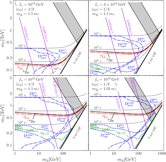
Now by confronting the stau yield with the maximum yield shown, e.g., in Figs. 11 and 12, we obtain the regions in the parameter space that are disfavoured by the hadronic BBN constraints associated with the abundances (47) and (48) [39]. For characteristic values of the thermal relic yield (28) and for (30) satisfying by construction, those regions are the ones enclosed by the short-dash-dotted (blue) lines in Figs. 13 and 14, respectively. As a guidance, dotted lines are shown to indicate , and in Fig. 13 and , and in Fig. 14. In fact, we limit our consideration of the hadronic BBN constraints to parameter regions with .
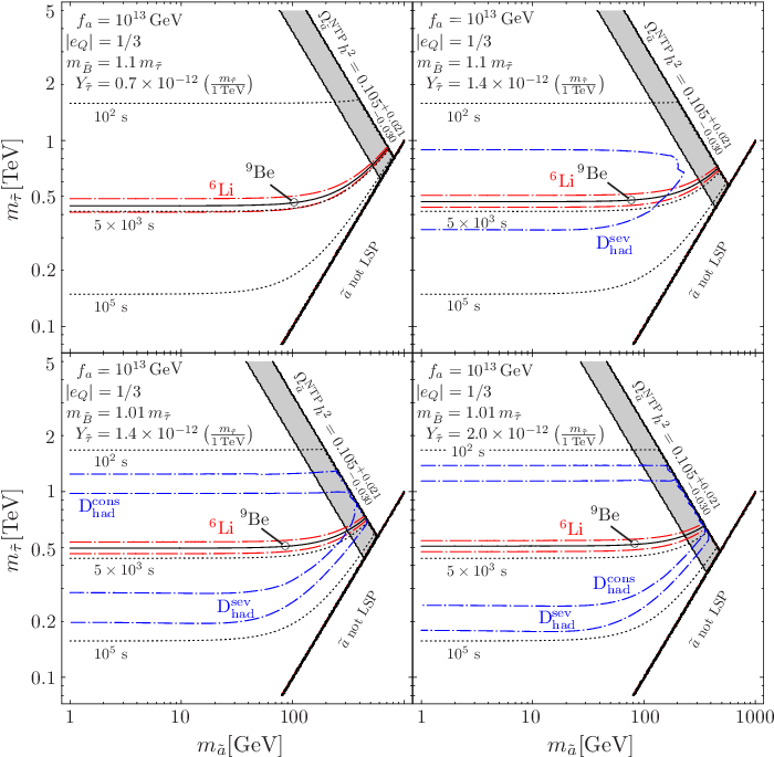
In Fig. 13 we have chosen the parameters such that the constraints shown in the panels become progressively more limiting. For the generic case of and a thermal relic yield (28) characterised by , both the severe and conservative hadronic BBN limits are still absent for (top left panel). For a larger thermal relic yield given by , accounting for a possible stau–slepton coannihilation, more severe constraints are obtained. In fact, the severe one associated with (47) disfavours a stau mass between 300 and 900 GeV for (top right panel). Decreasing disfavours also larger regions of parameter space due to the increase in illustrated in the lower panels of Fig. 10. Accordingly, for the same yield characterised by but now accounting for a possible stau–bino coannihilation with , the conservative constraints associated with (48) appear for the first time (bottom left panel). In the extreme case of having simultaneous bino–stau–slepton coannihilation with and , one encounters the most restrictive case shown in that figure. There the severe D limit disfavours almost the entire parameter space with (bottom right panel).
In Fig. 14 both the severe and the conservative hadronic BBN constraints already show up at and disfavour increasingly larger areas of parameter space in the panels for and . This is due to the rather large stau yield (30) that must be assumed at small to fulfil . The dependence of the yield (30) explains also the significant variation of the hadronic BBN constraints with . In contrast, those constraints do not change for when varying in case of a thermal relic yield (28) as can be seen in Fig. 13.
Electromagnetic BBN constraints have been explored in our study in close analogy to the hadronic ones. However, we condense the discussion since those constraints become relevant only for , i.e., in a region already disfavoured by the CBBN constraints discussed below. To determine the electromagnetic BBN constraints, we work with the -dependent upper limits on imposed by the primordial abundances of and by 3He/D. In particular, we consider severe and 3He/D constraints inferred from the respective limits given in Fig. 42 of Ref. [69] and a conservative constraint inferred from the respective limit given in Fig. 6 of Ref. [111]. The electromagnetic energy release is governed by the tau emitted in the 2-body decay with an energy in the rest frame of the . As each decays into at least one , which does not interact electromagnetically, only a fraction of contributes to the total electromagnetic energy injection [119, 90]. We use the conservative estimate
| (51) |
to avoid that the electromagnetic BBN constraints presented are overly restrictive. Proceeding as outlined for the hadronic BBN constraints above, we then obtain upper limits on the stau yield prior to decay. For the settings considered in Fig. 13, we find that the thermal relic yields (28) respect the obtained limits in the shown parameter space such that no electromagnetic BBN constraints appear in that figure; see also Fig. 5 in Ref. [39]. This is different in Fig. 14 where we encounter electromagnetic BBN constraints in the panels with . There the -imposed constraints disfavour the regions enclosed by the short-dashed (blue) lines and the 3He/D-imposed ones the regions enclosed by the double-dash-dotted (green) lines. However, we see in Fig. 14 that these constraints only show up in the regions well within those already excluded by the CBBN constraints, which will be discussed next, and are absent altogether for .
For the alternative and NLSP cases, the electromagnetic BBN constraints will look somewhat different. This is expected from the different properties of the respective emitted lepton; cf. Sec. 2.2 of Ref. [90]. For example, in the NLSP case, the electromagnetic energy release is instead of (51) since the electron does not decay. However, we refrain from a further detailed assessment since the resulting electromagetic BBN constraints will still be less restrictive than the CBBN constraints for scenarios with the NLSP or the NLSP.
Let us now address CBBN constraints on axino LSP scenarios with a long-lived stau NLSP [35]. At cosmic times , the presence of negatively-charged ’s can lead to the formation of and bound states once the rate of photodissociation of those bound states drops below the Hubble expansion rate. Then, depending on the and abundances at the relevant times, which are governed by and , primordial and production can become efficient via the following CBBN reactions [45, 46, 47]88 8 The large -production cross section reported and used in [46, 47] has been questioned by [120], in which a 4-body-model study is announced as work in progress to clarify the efficiency of production.
| (52) | ||||
| (53) | ||||
| (54) |
Here we work with the observationally-inferred limits on the respective primordial fractions of [111, 121, 122] and [47],
| (55) | |||||
| (56) |
and obtain the CBBN constraints by confronting with the limits in Fig. 5 of Ref. [47].
In Figs. 13 and 14, the CBBN constraints associated with the range (55) are indicated by pairs of long-dash-dotted (, red) lines and the ones associated with (56) by solid () lines. The regions below those lines are disfavoured by an excess of and above the respective limits. As seen in Fig. 13, the CBBN constraints on scenarios with a thermal relic yield (28) follow contours of constant and become independent of for . In fact, we find that the CBBN constraints disfavour and that they show only a mild dependence on in contrast to the hadronic BBN constraints. For the yield (30), the CBBN constraints can disfavour even smaller of about (cf. Fig. 14) as they become more restrictive towards smaller due to the significant increase of .
Here one should also comment on the potential interplay between late energy injection and CBBN. We use the CBBN limits from Ref. [47] which have been derived for a abundance obtained with SBBN. For an increased abundance resulting from hadrodissociation of , CBBN of and becomes even more efficient. For , this is evident since its catalysis proceeds via (52) and since the primordial abundance of stays significantly below the one of at the relevant times (even for a maximum of observationally tolerable hadrodissociation of ); cf. Fig. 2.4 in Ref. [123]. For , an increased output results from the final step of its catalysis (54), which becomes more efficient since an enhanced abundance of increases the number of neutrons at the relevant times [124]; cf. Fig. 4 in Ref. [47]. Moreover, the debris of hadrodissociated can hit ambient and thereby fuse additional [70, 69, 60]. The interplay of late energy injection and CBBN will thus lead to constraints that can only be stronger than the ones presented in this work. Aiming at conservative limits, this allows us to neglect those intricacies which will have to be faced in future refinements of the presented constraints.
4.4 Comparison and Discussion of the Cosmological Constraints
Let us close this section with a brief comparative discussion of the cosmological constraints addressed in this work. We consider again cosmological settings with a thermal relic stau yield (28) and such with (30) satisfying by construction.
When presenting Fig. 13, negligible was assumed and thereby and . While the shown BBN constraints are not affected by this assumption, significant additional parts of the parameter space can be excluded by the dark matter constraint (23) for , as explicitly illustrated in Fig. 8. With thermally produced axinos dominating , which are compatible with cosmic structure formation down to as low as or even smaller (cf. Sec. 4.2), the structure formation constraints shown in Fig. 9 do not apply. In other cases with and a thermal relic stau yield (28), those constraints apply within the grey bands shown in Fig. 13. However, they are still relatively mild. For the upper (lower) panels, it can be seen in Fig. 9 (Fig. 14, bottom right panel) that only the most restrictive velocity limit (35) disfavours parts of the grey bands for (). Moreover, the contributions to at are typically very small and clearly compatible with current limits for thermally produced axinos and for those from decays of thermal relic staus with described by (28).
In Fig. 14, in which given by (30) is used, is considered everywhere in the shown parameter space. This also implies negligible and thereby and . Moreover, here the constraints from structure formation associated with (34) and (35) apply not only in the grey bands but disfavour the regions to the left of the respective solid (purple) diagonal lines. Accordingly, even the conservative structure formation constraint associated with (34) is significantly more restrictive than both the constraint (31) with imposed by our working hypothesis of a standard thermal history and the BBN constraint (45) with at . In the regions with larger that are allowed by the respective structure formation constraint, the hadronic BBN constraints are often the most restrictive ones. While those become weaker for , the CBBN constraints become increasingly more restrictive in that region which is associated with larger values due to phase-space suppression of the stau decays. As already mentioned, the electromagnetic BBN constraints show only up for and only in parts of the parameter space already disfavoured by the CBBN constraints. We also show grey bands in Fig. 14 but merely as a guide to show where the stau yield (30) coincides with that of the stau thermal relic yield (28) with or (first three panels) and with or (bottom right panel). Those are the regions in which one might consider (30) to take on its most natural values, i.e., values motivated by thermal-freeze-out considerations.
Looking once more at Fig. 13, one finds that the hadronic BBN constraints are much more sensitive to the stau yield and the ratio than the CBBN constraints. While the CBBN constraint disfavours basically in all four panels, the hadronic BBN constraint may not show up at all or may disfavour even significantly larger values of or above, depending on and the ratio. Indeed, this sensitivity motivated us to show those four combinations of and accounting systematically for the possibilities of no coannihilation, stau–slepton coannihilation, stau–bino coannihilation, and simultaneous stau–bino–slepton coannihilation. While is fixed to in Fig. 13, an illustration of the dependence of the CBBN constraints can be found in Fig. 4 of Ref. [35] and in Fig. 5 of Ref. [39] which also includes hadronic and electromagnetic BBN constraints. For and , those figures demonstrate that BBN constraints start to become an issue for while settings with smaller are free from those constraints when considering thermal relic stau yields and the limit from searches at LEP [10]. With being independent of and , even settings with up to will be free from BBN constraints if and .
Finally, there is the possibility that very light thermal relic axinos may exist as HDM while CDM is provided by axions [33]. Here the obtained limit from structure formation constraints is significantly more restrictive than the previously known limit imposed by the dark matter constraint (23). Interestingly, also for very light axinos the hadronic, electromagnetic and CBBN constraints apply since they are sensitive to the yield of the stau NLSP, its SM decay products and its lifetime, which is independent of in that regime. As mentioned, for given by (28), the location of those constraints can then be seen directly in Fig. 13 as they agree with the ones shown for .
5 Collider Phenomenology of Axino Dark Matter Scenarios
Cosmological considerations can significantly constrain the parameter space of SUSY axion models. Nevertheless, in order to investigate and to determine the properties of axinos, one must look towards laboratory experiments. Due to the axino’s highly suppressed interactions, its production cross sections at various colliders are very small. Instead, one would look for the NLSPs, the staus, either from direct pair production or from cascade decays of heavier sparticles. In fact, a first hint towards axino dark matter would come from the appearance of quasi-stable staus at the Tevatron, the LHC or future colliders.99 9 Collider studies of long-lived charged massive particles (CHAMPs), a category to which the staus belong, can be found for example in Refs. [125, 126, 127, 128, 129, 130].
The most straightforward property of the stau to determine would be its mass , which can be measured using time-of-flight (TOF) data from the muon chambers. At the LHC, it is estimated that this can be done with accuracy [131, 132]. In order to measure other properties, such as the stau lifetime and the axino mass , it is important to be able to study the stau decays. The approach that one should take to analyse these decays depends on the decay length and on the size of the detector . Here it is natural to distinguish the following three cases, which we now relate to the considered axino dark matter scenarios:
- •
If the lifetime is very short such that then the staus would effectively decay immediately after production. This decay length corresponds to . For the SUSY axion models considered in this paper, a stau with such a short lifetime can only be achieved with a very low and a very heavy stau, as well as larger than 1/3. For example, with the lowest value respecting (1), , one would need , along with , , and , to obtain . This very high stau mass is out of the reach of current and near future colliders. If one considers a stau mass that is more likely to be probed at colliders, while keeping , along with the selection of , , and , one obtains a lifetime of and .
- •
If the lifetime is such that then the staus will decay with a displaced vertex within the beam pipe or the detectors. With a typical detector size, , it is evident from the arguments given above that this case still requires a very low and a very heavy stau to be relevant for the considered axino LSP scenarios.
- •
If the decay length is , there would be only few in-flight decays within the detector and most of the staus would escape the detector. This is the case on which we focus in this section. It applies to axino LSP scenarios respecting (1) and with such that the stau NLSP can be probed at current or near future colliders.
There are different ways to access stau decays in the considered third case. For (still corresponding to decay lengths well over ), it has been argued that a substantial number of in-flight decays can still be observed within the detectors [133, 134]. Also for larger , decays could be accessible since the produced staus will be slowed down (due to ionisation energy loss) so that some of them are expected to be stopped within the main detectors [43, 135, 136] or in an additional dedicated stopping-detector [40, 41, 44].1010 10 Note that this method is not limited to staus with long lifetimes. It can also be used to study staus with very short lifetimes but highly boosted momenta. By recording the stopping point/time with those devices, it seems possible to study the subsequent decays of the trapped staus and to determine their lifetime. For very long lifetimes, there was also a suggestion to place a water tank around the detector to trap the staus, such that the water can be moved to a different location at a later date for further analyses [42]. Even the surrounding rock has been suggested to be used for the study of stau decays [137].
In the coming parts of this section we first explore the prospects of stopping staus and studying their 2-body decays with the main detectors at the LHC and the ILC, i.e., without additional stopping-detectors. Four benchmark scenarios are proposed and studied for this purpose. Thereafter, we turn to the 3-body stau decays into the LSP, a tau and a photon, whose study might require additional stopping-detectors. Based on those decays, we address the possibility to distinguish between the axino LSP and the gravitino LSP at colliders.
5.1 Probing 2-Body Decays of Trapped Staus at the LHC and the ILC
To illustrate the potential of stopping staus and analyzing their 2-body decay into the axino LSP at the LHC and the ILC, we consider the four SUSY benchmark points specified in Table 3. To simplify matters and minimise the number of parameters that have to be specified, we work in the framework of CMSSM. Here the gaugino masses, the scalar masses and the trilinear scalar interactions are assumed to take on the respective universal values , and at the scale of grand unification . Specifying also the mixing angle in the Higgs sector and the sign of the higgsino mass parameter , one can calculate associated mass spectra at the weak scale and stau yields prior to decay. For the considered benchmark points, we obtain those quantities by employing the spectrum calculator SuSpect [138] and MicrOMEGAs 2.4 [139, 140] for . Those tools are also used to verify that the accelerator constraints are respected for our chosen points.
| Scenario | [GeV] | [GeV] | [GeV] | [GeV] | [GeV] | ||
| A | 170 | 560 | 30 | 210.3 | 232.4 | 270.1 | 0.73 |
| B | 50 | 550 | 8 | 207.6 | 226.8 | 212.4 | 1.34 |
| C | 138 | 435 | 25 | 174.3 | 177.7 | 215.6 | 1.42 |
| D | 135 | 700 | 6 | 290.2 | 292.6 | 292.8 | 1.94 |
We have chosen the benchmark points such that they fall into the classes for which we studied cosmological constraints in Sec. 4. This can be seen in Table 3, where values specify the associated stau yield given by (28) with the respective values. Scenario A shows no coannihilation, B stau–slepton coannihilation, C stau–bino coannihilation and D simultaneous stau–slepton-bino coannihilation; cf. text below (28). These four scenarios come with a bino-like lightest neutralino and with lighter staus that have left-handed component. This left-admixture can be reduced further by fine-tuning the parameters or considering other SUSY scenarios that offer greater flexibility in choosing parameters. In fact, we use our result for the stau lifetime derived for right-handed staus in Sec. 3 also for the four benchmark points even if they show a non-negligible left-right mixing.
The SUSY hadronic axion model is not part of the CMSSM and the associated parameters have to be specified in addition to those in Table 3. For concreteness, we choose , , and . While this scenario respects all constraints from structure formation and BBN, the dark matter constraint limits the maximum reheating temperature to a relatively low value of about ; cf. Fig. 8 and associated explanations given in Sec. 4.1. For smaller and/or larger , this limit would be more relaxed. Note also that a change in will not noticeably affect the stau lifetime and the associated error derived below, as long as . However, the same is not true for a change in , on which the stau lifetime strongly depends; see (10).
Let us now turn to the LHC. As mentioned above, we concentrate on the fraction of staus that are produced with small enough values of such that they lose enough kinetic energy through ionisation to be stopped within the main detectors. For this setting, the authors of [135] suggest the possibilities of having a trigger for a beam dump should a stau be detected to have stopped, such that its subsequent decay can be observed, or of studying the decays of the staus during beam downtime.1111 11 Another recent LHC proposal [136] suggested to measure the lifetime of staus trapped in the ATLAS detector during scheduled shutdown periods. It is thus more suitable for studying staus with a very long lifetime of several days or more. However, in the scenarios that we are considering, a lifetime longer than about three hours is disfavoured by the CBBN constraints discussed in Sec. 4.3.
Our LHC study follows closely the approach of Ref. [135]. Using Pythia 6.4 [141] and the cuts 1–4 outlined in [135], we have generated proton–proton collision events with a centre of mass energy and an integrated luminosity for each CMSSM point given in Table 3. The resulting spectra are shown in Fig. 15.
Following the strategy outlined in [135], we consider only the staus produced with as those that get trapped in the calorimeters of the ATLAS detector. For the considered benchmark scenarios, we list the corresponding numbers of staus expected to be stopped in the ATLAS calorimeters, , together with the right-handed up squark mass , the gluino mass and the total SUSY production cross section in Table 4.
Scenario [GeV] [GeV] [pb] A 1127.2 1272.8 0.66 119 5.4 0.8 B 1097.5 1250.3 0.76 182 5.8 0.6 C 896.4 1008.3 2.60 522 10.8 0.7 D 1372.1 1563.6 0.185 58 2.5 0.5
Clearly is larger for larger ,1212 12 Table 4 lists leading order results for . The values increase by factors of 1.2–1.4 when including the next-to-leading-order SUSY-QCD corrections so that may be above the given estimates. and thus governed by and at the LHC.
The lifetime of the trapped staus is determined by measuring the time between when the stau is stopped and when its subsequent decay is detected, where we refer to [135] for details on the different techniques one would use for different . By extrapolating the results of [135] to our parameter points, we obtain the expected statistical 68% CL precision of the determination listed in Table 4. Clearly the statistical accuracy depends on the number of events that can be observed, and at the LHC, this is very much dictated by the mass spectrum of the SUSY scenario that is realised. With the conditions assumed for the generation of the above events, light squarks and gluinos with masses would be preferred for a statistical 68% CL accuracy of the determination of .
A similar analysis can be done for a future linear collider. In Ref. [43] it has been proposed to use the Large Detector Concept (LDC) [142] at the ILC to study the decays of the trapped staus. The staus produced in the collisions can become trapped either in the hadronic calorimeter or the yoke of the LDC. We follow very closely the strategy of [43] to determine the statistical accuracy with which the properties of the stau and the axino can be determined.
Again using Pythia 6.4 [141], we now generate electron–positron collision events with a centre of mass energy of and an integrated luminosity of for each CMSSM point given in Table 3 . The obtained distributions for the produced lighter staus are shown in Fig. 16.
In addition to the total distribution (solid line, red), we illustrate the contributions of the following processes to the production of lighter staus: (plus signs, green), (crosses, blue), (stars, magenta), (boxes, cyan), and (circles with crosses, yellow), and (open circles, black) and (filled circles, orange). This breakdown of the contributing processes allows us to see effects associated with small mass differences between the lighter stau and the sleptons , and/or the lightest neutralino : Pronounced peaks just below the ones from direct production come from cascade decays of and at point B (top right panel), of at point C (bottom left panel) and of , and at point D (bottom right panel). In addition, one finds also for points A and B that a significant fraction of the staus is produced in decays of the lightest neutralino . This indicates that a lightest neutralino with a mass close to the one of the lighter stau would be beneficial for phenomenological studies.
Following Ref. [43], we have calculated the numbers of staus expected to be stopped in the hadronic calorimeter, , and in the yoke, , of the LDC. For the CMSSM points A–D, the results are tabulated together with the total SUSY production cross section in Table 5. The respective ranges for which the staus are expected to get stopped in those detector parts depend on and are typically – (hcal) and – (yoke) for our benchmark points; see also Table 2 in Ref. [43].
| Scenario | [fb] | [GeV] | [s] | [GeV] | ||
| A | 84 | 508 | 1362 | 210.3 0.2 | 5.4 0.2 | 10 64 |
| B | 190 | 681 | 1311 | 207.6 0.2 | 5.8 0.2 | 10 58 |
| C | 310 | 1569 | 2933 | 174.3 0.1 | 10.8 0.3 | 10 35 |
| D | 3.6 | 0 | 0 | 290.2 0.2 | 2.5 0.1 | 10 53 |
Note that and depend not only on but are also very sensitive to the specific shape of the distribution, which is governed by the mass spectrum and the considered . In particular, for scenario D and , almost all the events are clustered around the – region, as can be seen in the bottom right plot of Fig. 16. The momenta would thus be so low that the staus do not have enough energy to reach the LDC hadronic calorimeter/yoke. Nevertheless, they are energetic enough to travel out of the beam pipe and become trapped in the inner detectors. We thus treat all the staus produced, 1814, as stopped to derive the expected and accuracies listed for scenario D. This is different for the scenarios A–C where we use and to infer those accuracies. Here we should note that a future linear collider will have a tunable centre of mass energy . This will allow us to maximize the number of staus stopped in those detector parts most suitable to study the decays. However, such optimisations for scenarios A–D are beyond the scope of this work and left for future studies.
Independent of the stopping of staus, the kinematics from the direct production of stau pairs will allow for a determination the stau mass with an accuracy listed in Table 5. As shown, we expect that the stau mass can be measured very precisely at the ILC, with an error below for all four CMSSM points. This can perhaps be further improved on if combined with a mass extraction using TOF data. The measurements are not expected to be that accurate, but greatly improve with increasing numbers of trapped staus as can be seen in Table 5. Accordingly, these measurements would benefit from the optimisations mentioned above. However, the statistical accuracy of the determination expected to be achievable at the ILC is already very promising at this stage.
For scenarios A–C, the explored measurement of the stau lifetime utilises the staus trapped both in the hadronic calorimeter and the yoke, while only those trapped in the hadronic calorimeter are considered when probing the axino mass. This restriction results from the fact that the axino mass exploration relies on the kinematics of the 2-body decay ,
| (57) |
and thereby on the determination of the energy of the emitted tau lepton [37]. With being the maximum energy of the observable decay products, the latter requires to study the endpoints of the energy spectrum of the emitted ‘ jets’ and thus a hadronic calorimeter [43]. As shown in Table 5, only rough upper limits on are expected for . This is due to the difficulties to determine with sufficiently high precision. While the situation will improve for , it will be even worse for smaller values because of the demand for an even more precise determination.1313 13 In a more general setting than the CMSSM, it may also be the that is the NLSP. Then it will be easier to achieve the precision required to probe smaller values since this relies now on a measurement of the energy of the electron that is emitted (instead of the unstable tau) in the decay .
Measurements of the values of , , and can be used to approximately constrain the PQ scale [37]. Here the dependence becomes only relevant in the region, where one should be able to infer with a better accuracy than reported in Table 5. Using the LL expression (21), we find that only the following combination can be probed by measuring , , and at colliders
| (58) |
where one sees explicitly that the dependence becomes negligible for . Note that it will not be possible to constrain alone from collider data. For the considered SUSY axion models, always appears as the ratio in the prefactor of the decay widths and as the product in the logarithm; see (11) and (13). However, ongoing and future axion searches might yield valuable additional insights into the axion model possibly realised in nature as detailed, e.g., in Sec. 6 of Ref. [35]. In fact, an axion discovery via the axion–photon interaction (7) may point to and . To some extent, ambitious precise future measurements of , , (and ) at colliders could then probe via (58) and thereby – as advertised in the last paragraph of Sec. 3.1 – the hierarchy between and the heavy (s)quark masses .
5.2 Distinguishing between Axino LSP and Gravitino LSP
Should a long-lived charged massive particle be detected at a collider, it is not guaranteed that its decay products include an axino. Despite being able to accurately determine the NLSP’s lifetime and other properties, there can remain ambiguities over the identities of its non-SM decay products, i.e., the LSP. In particular, as mentioned at the end of Sec. 2, the gravitino is also a well-motivated LSP candidate in SUSY scenarios that include gravity. Similarly to the axino, it is very weakly interacting so that a long-lived stau NLSP can also occur naturally in gravitino LSP scenarios. Here the stau NLSP lifetime is governed by a 2-body decay which proceeds via a supergravity coupling [51]
| (59) |
where the gravitino mass does not only enter via the kinematics but also governs the interaction strengths via the spin-1/2 goldstino components.
Comparing (59) with given by (10) in the axino LSP case, agreement between the stau NLSP lifetimes in both scenarios is found on the lines shown in Fig. 17.

For concreteness, we consider and (solid lines) or (dashed lines). Those masses may be known quite precisely from collider studies when will be measured. Indeed, the LSP mass or will be much harder to probe (cf. Table 5) and also might still not be more strongly constrained than summarised by (1). To account for the potential additional dependence, the agreement is indicated for the two representative cases (lower lines) and (upper lines), whereas is kept fixed. In the limit , we find that
| (60) |
in (59) gives the same stau NLSP lifetime as the LL result (21) in the axino LSP case.
The smaller or , the shorter is the stau NLSP lifetime. Accordingly, one finds a lower limit imposed by (1) in the axino LSP case. In Fig. 17 (, ), this lower limit ranges between (for and ) and (for and ). Much smaller are possible with a light gravitino LSP, , and could as such provide hints against the axino LSP. In Ref. [37] it had been pointed out that and will point to a gravitino LSP scenario. While we agree on the short lifetime being a potential indicator for the gravitino LSP, the mentioned long lifetime cannot exclude the axino LSP since may well be larger than considered in [37]. Instead, we find that the upper limit imposed by CBBN for typical yields (28) applies for both LSP candidates. The additional constraints from hadronic energy injection might tighten this upper limit but differently for the gravitino LSP (see [143, 47]) and the axino LSP (see [39] and Sec. 4.3 above).
Another way in which one can try to distinguish between an axino LSP and a gravitino LSP is by studying the 3-body decay of the stau [37, 44]. In Ref. [37] the authors focused on the branching ratio of the integrated 3-body decay rate and on the double differential distribution of the 3-body decays. For the axino LSP case, our result of the latter quantity is given in (13) above and also used to calculate that branching ratio (16) with results illustrated in Fig. 3. Also Ref. [44] considered the branching ratios of the 3-body decays in the following form and with the given choice of cuts,
| (61) |
Here we present an updated comparison of both the double differential distributions
| (62) |
and of (61) using the results of our calculations of the 2- and 3-body decays of the stau NLSP into the axino LSP presented in Sec. 3. For the 3-body decay of the stau NLSP into the gravitino LSP, we use the result obtained in [37], which is applicable for finite .1414 14 In Ref. [144] the decay was also considered but in the limit .

The darker shadings correspond to higher number of events, with the contours representing the values 0.2, 0.4, 0.6, 0.8, 1.0, 1.5 and 2.0. The first three panels show the axino LSP case for , , , and for different values of (top left), (top right) and (bottom left). The lower right panel shows the gravitino LSP case for and . This value of is chosen such that one finds an agreement of the stau lifetime in the two scenarios considered in the bottom panels; cf. (60). We however note that changes in , while significantly altering the stau lifetime, do not greatly affect the shown differential distribution as long as . Likewise, changes in the values of and cause only slight changes of the distributions.
To varying degrees, all the panels show a preference for producing soft and collinear photons. The top right panel is the scenario most closely resembling the plot shown for the axino LSP case in Fig. 5 of Ref. [37]. Here we find an excess of events for highly energetic photons produced back-to-back to the emitted taus in comparison to what is obtained in the corresponding gravitino LSP case (cf. Fig. 5 of [37]). This is in agreement with the result found in [37], and we now note how this excess region changes for different values of the bino–stau–mass ratio . For smaller , the excess is more pronounced with events covering a phase space that extends towards larger values of as can be seen in the top left panel of Fig. 18. This is due to the one-loop decay mode, shown in Fig. 2 (a), being more dominant over the two-loop decay mode in that region as the bino becomes more and more on-shell. In turn, towards larger values of , the excess region shrinks such that for (bottom left panel) the excess region is basically missing altogether. In the gravitino LSP case, (62) is less sensitive to with more events expected in the very hard photon region for larger . It must be noted however that this increase is very marginal and would require high statistics to be noticeable. Thus, the larger the ratio, the more difficult it becomes to differentiate between the axino LSP and the gravitino LSP. This is shown explicitly in the bottom panels of Fig. 18. Here we have chosen parameters for the gravitino LSP case to most closely resemble phenomenologically the axino LSP case to its left to test a particularly difficult situation: and, as already mentioned, such that agrees in the lower panels. If we look closely at those two distributions, we find small differences, with the axino LSP scenario having a larger phase space area with small values of (62). However, these differences are small and we would need large statistics and precise measurements to rely on them for a distinction between the two scenarios.
To give an idea of the numbers that can be expected, we assume trapped staus whose decays can be observed in a detector component (such as a hadronic calorimeter) that allows for the analysis of the 3-body decays. This may seem somewhat optimistic in light of our estimates (obtained without exploring ILC-parameter optimisations) given in Table 5. Nevertheless, even could be feasible at the ILC already without additional stopping-detectors [43]. Also at the LHC one might be able to stop the assumed number staus but only when invoking additional stopping-detectors [41, 42, 44]. For example, with massive stoppers set up next to the Compact Muon Solenoid (CMS) detector at the LHC, it seems possible to stop staus with up to and to achieve values that are more than an order of magnitude above the ones reported in Table 4 above [44]. Now, for 5000 trapped staus, we expect to see 149(stat), 58, 26 and 28 3-body events with and when considering the scenarios in Fig. 18 in the sequence of left to right and top to bottom, respectively. Looking at the region with and , in which an excess of events may be found, we would expect 53(stat) (36% of the above number of 3-body events), 19 (33%), 0.3 (1.4%), 0.4 (1.4%) events, respectively. Clearly, this looks very pessimistic for distinguishing between the axino LSP and gravitino LSP scenario with . If we enlarge the phase space region to while keeping , we would obtain 0.7 (3.5%) and 1.5 (5.2%), respectively, for these two cases. Admittedly the improvement is not large, but in lieu of other signals, this discrepancy could be indicative.
In the axino LSP case, the markedness of the potential excess of highly energetic photons produced back-to-back to the emitted taus is not only sensitive to but also to the size of the logarithm . As can be seen in (13), the smaller this logarithm, the larger is the relative importance of the one-loop 3-body decay mode shown in Fig. 2 (a) and thereby the number of excess events. This can affect the success of the distinction between the axino LSP and the gravitino LSP in a way that we now illustrate by establishing a connection to the results of Ref. [44].
In Ref. [44] the branching ratios (61) and distributions in intervals were explored based on the 2- and 3-body decay widths calculated in [37]. Accordingly, the results for the axino case did rely on a particular choice of , where the factor and the mass scale were introduced to parametrise the uncertainty associated with the cutoff procedure applied in [37] instead of the two-loop calculations presented by us in this work; see also Sec. 3.2. In particular, in the comparisons of (61) in [37, 44], was fixed and different choices of including [37], 0.5, 0.75, 1 and 2 [44] were considered. Relying on our 3-body result (13) and on the 2-body rate in the LL approximation (21), we can now relate those choices to the parameters of the underlying model:
| (63) |
The different scenarios considered in [37, 44] can thus be related to combinations of and for a given . For example, with , () is found for and ( and ), while would require and/or . With such relations in mind, the results for – shown in Figs. 16–20 of Ref. [44] apply also to our considerations. There it has been estimated, e.g., that () would be sufficient for () to establish a difference between the branching ratios (61) when and , while the required increases to about () for . For further results and details, we refer to Ref. [44] and to relation (63) for the mapping to parameters of the SUSY axion models considered in this work. Note however that relation (63) is only relevant for making contact with the phenomenological investigations of [37, 44]. When the logarithm is not fixed to a number such as , agreement of our 3-body result (13) and of the 2-body rate in the LL approximation (21) with [37] is found for , and , as already discussed in Sec. 3. Still the size of will be relevant for the viability of the axino–gravitino LSP distinction as illustrated by the results of Ref. [44] as mentioned above.
6 Scenarios with
In the above sections, we mainly considered the axino LSP scenario with a stau NLSP, where . In Sec. 5.2 we also considered the hierarchy (or equivalently, a SUSY scenario with no PQ extension) in the context of differentiating the experimental signatures of an axino LSP and a gravitino LSP. Now limiting ourselves to the hierarchy , yet another two orderings of the masses are possible, and , as already mentioned in Sec. 2. We will explore the consequences of both of these in this section. In particular, we consider effects on decays and the lifetime of the lighter stau, on cosmological constraints and on collider phenomenology.
Scenarios in which both the axino and the gravitino are lighter than the other sparticles (cf. [26, 27]) have been considered first in studies aiming at the understanding of structure formation and of the matter power spectrum [145, 146, 147]. Moreover, it had been realised that such a spectrum may provide a solution to the gravitino problem of thermal leptogenesis [77]; see also [63, 72, 148, 149]. Such a setting may also allow for a late non-standard increase of after BBN but before the beginning of structure formation [150]. Brief comments on scenarios were already given in Refs. [37, 35]. We now elaborate on those and provide several new insights, where our focus is on the behaviour of the lighter stau and on associated constraints and phenomenology, see also Ref. [63].1515 15 As this work was being finalised, a study of constraints in scenarios with the gravitino LSP and the axino NLSP appeared [151], which is complementary to our considerations.
6.1 Lifetime and Branching Ratios
Let us first take a look at how the lifetime of the stau is affected. In addition to the 2-body decay , the 2-body decay is also kinematically viable. The lifetime of the stau is then governed by these 2-body decays:
| (64) |
with the partial decay widths (10) and (59). For given and , the relative importance of the different 2-body decays depends on and , which govern and , respectively. This is illustrated in Fig. 19 for , , , and , where the latter limit minimises the dependency of on .
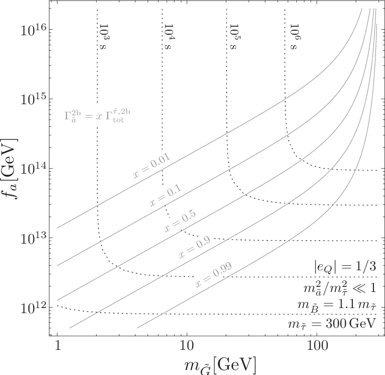
The dotted lines indicate contours of the stau lifetime and the solid grey lines the fractional contribution of to the total 2-body decay width of the stau: . Note that the upward bending of the contours towards larger results from the factor in , cf. (59), which also accounts for the phase space suppression of the decay for . Above (below) this contour, the stau decays dominantly into the gravitino (axino), which explains the clear turning points in the shown lifetime contours.
For , both 3-body decays contribute simultaneously to . Accordingly, the corresponding branching ratio with cuts is given by
| (65) |
with (15) and the corresponding result of Ref. [37]. In Fig. 20 (a) this branching ratio is illustrated by the dotted lines for the same parameters as in Fig. 19 and for and , as in Sec. 5. The shown contours vary only between 0.8% and 1.5% and confirm that the total stau decay width is governed by the 2-body decays. The solid grey lines show the fractional contribution of to the total 3-body decay width of the stau: . One finds that dominates in a range that is slightly larger than the one in which dominates in the 2-body case (see Fig. 19).


(a) (b)
Figure 20 (b) shows the corresponding 4-body branching ratio (dotted lines)
| (66) |
where
| (67) |
with (20) and the corresponding result of Ref. [90]. Here we set , as in Sec. 4.3, and the other parameters again as in Figs. 19 and 20 (a). Now the solid grey lines show the fractional contribution of to the total 4-body decay width of the stau: . One can see that dominates in a () region that is even a bit larger than the one in which dominates in the 3-body case. Moreover, the shown contours range between 0.04% and 0.16%. This demonstrates that the 3-body decays considered in panel (a) are about an order of magnitude more abundant than the 4-body decays considered in panel (b).
6.2 Cosmological Constraints
Let us now turn to the cosmological constraints from primordial nucleosynthesis for characteristic freeze-out yields of the lighter stau described by (28). Indeed, the freeze-out yield of the lighter stau prior to decay is not affected by the presence of a light gravitino. Also decays such as or, alternatively, , even if taking place after freeze out and prior to decay of the stau, will not dilute as the emitted extremely weakly interacting particles will not thermalise and not affect the entropy density. However, we have just seen that can be very different for , and this will affect the CBBN constraints and also the BBN constraints associated with late hadronic and electromagnetic energy injection. Moreover, there are now the additional decays and contributing to . Accordingly, we find
| (68) |
with given in (64), and that the conservative estimate (51) changes to
| (69) |
where the energy of the tau emitted in and is given respectively by
| (70) |
The resulting constraints are illustrated in the – plane in Fig. 21 for (a) and (b) , with the other parameters set to , , , and the yield .


(a) (b)
For orientation, we show contours of , , and (dotted lines) and of , and (solid grey lines). In the region with , the (C)BBN constraints are insensitive to and basically as in the case considered in Sec. 4.3; see also Fig. 5 (a) of Ref. [39]. In turn, in the region with , the shown constraints are insensitive to and basically as in the LSP cases with or no PQ extension; cf. Fig. 6 of Ref. [47].
Let us now describe the (C)BBN constraints shown in Fig. 21. The regions to the right of and above the long-dash-dotted (red) and the solid lines are disfavoured by the CBBN constraints associated with (55) and (56). Again, these lines are located close to the contour (not shown). The hadronic BBN constraints associated with (47) show up in panel (b), where they disfavour the region enclosed in the L-shaped strip bounded by the two short-dash-dotted (blue) lines. These severe constraints do not appear in panel (a), and also the conservative constraints associated with (48) are absent in both panels, which is consistent with Fig. 5 (a) of Ref. [39] and Fig. 6 of Ref. [47]. The electromagnetic BBN constraints lie well within the region already disfavoured by CBBN in our panels (a) and (b). Here the constraint disfavours the regions above the double-dash-dotted (green) line. Moreover, in panel (a) the constraint disfavours the regions between the two leftmost dashed (blue, ) lines and to the right of the corresponding 3rd line from the left-hand side or the region above the rightmost of those lines (), whereas in panel (b) the regions to the right of the leftmost dashed (blue, ) lines and the ones to the right of the corresponding rightmost (broken, ) line are disfavoured.
We find that the upper limits on , which have been obtained for a given in the gravitino LSP case and which imply upper limits on the SUSY breaking scale [143, 47], hold only in the parameter region with , i.e., for . For , the gravitino mass range becomes cosmologically viable with a standard thermal history, R-parity conservation and a standard freeze-out yield . Despite a then relatively small branching ratio of the decay, this might still be relevant for collider phenomenology since a kinematic determination appears to be feasible only in that mass range [144, 43, 44] which is disfavoured otherwise [143, 47]. On the other hand, our upper limits on obtained for a given and [35, 39] hold only in the parameter region with , i.e., for . If , values even as large as will not be cosmologically disfavoured.
So we see that the scenario opens up regions of parameter space that are disfavoured if only the axino [35, 39] or only the gravitino [90, 143, 47] is lighter than the stau. Accordingly, without additional phenomenological insights into or from collider experiments or axion searches, it will not be possible to infer rigid upper limits separately on or once and are known, even under the assumption of a standard thermal history. In fact, for known and and with inferred for a standard thermal history with , we think that a figure such as the ones shown in Fig. 21 will be the ideal way to display the possible (C)BBN constraints on and/or for a given axion model.
Before proceeding we also note that some of the constraints disfavour regions for that were previously free of constraints. For example, the electromagnetic and hadronic BBN constraints in the LSP cases with or no PQ extension disappear for a finely tuned – degeneracy leading to . For and no additional finely tuned – degeneracy, this is no longer the case since will be governed by (51) and (49) which can remain sizeable. Accordingly, the and constraints shown in Fig. 21 do not disappear for .
6.3 Collider Phenomenology
Not only the cosmological constraints but also collider phenomenology is affected by the possible mass hierarchy considered in this section. The methods to probe and will remain the same. Also our estimates of , and in Sec. 5.1 will not change for the assumed values. However, the experimental distinction between the axino LSP and the gravitino LSP faces additional complications. While brief comments on this issue had already been given in Secs. 1 and 4.3 of [37], we now address this issue more extensively and in more detail, with a number of additional insights.
Even with the axino being the LSP, a short stau lifetime of is now possible for due to . Then such will no longer provide a hint against the axino LSP (cf. Sec. 5.2) but point to a light gravitino, with the possibility of an even lighter axino. Moreover, we have shown explicitly in Fig. 20 (a) that both and is possible, whereas the corresponding regions (i.e., and ) in parameter space are mainly governed by and . Accordingly, double differential distributions such as the ones shown in the top panels of Fig. 18 do not necessarily point to the axino LSP if . Instead, they then would point to a parameter region such as the one with in Fig. 20 (a), on which cosmological constraints can be imposed as shown in Fig. 21. The 3-body decays can thereby still provide very valuable information. Since the region with in Fig. 20 (a) basically coincides with the region in Fig. 19, an experimental signature for implies and thereby that the stau decays into the axino govern . This would mean that a measurement would probe the PQ scale , as outlined in (58) for the considered SUSY axion models. In turn, the opposite case with would mean that a measurement would probe the gravitino mass (and thereby the SUSY breaking scale), provided as inferred from Newton’s constant.
Note that a measurement alone will point to a contour in the – plane; cf. dotted lines in Figs. 19 or 21. Such a contour can then be confronted with cosmological constraints. However, as can be seen in Fig. 21, the most restrictive and thereby relevant constraints basically follow the shape of the contours. Thus, the cosmological constraints cannot tell us whether is governed by stau decays into the axino or the gravitino or by both. It will then still be unclear whether a measurement probes or or a combination of both.
Axion searches and resulting limits on may help in particular for small values of . Already the current limit (1) will point to if –, where the given range of the upper limit reflects an uncertainty with respect to the axion model and here the parameters and ; cf. Sec. 5.2. In the future, the lower limit may increase and thereby also the above values of the limit. Alternatively, a future axion discovery may point to an value and also to an value (cf. Sec. 6 of [35]). Those values together with measured , and can then be tested with relation (58). For a reasonable value, which appears only in the logarithm and which will be difficult to probe independently of the stau decays (cf. end of Sec. 5.1), an agreement would then point to and thereby to the -independent part of the contour; cf. dotted lines for in Fig. 19 or 21. In turn, a severe mismatch in (58) may originate from for which is governed by and independent of ; cf. dotted lines for in Figs. 19 or 21.
Additional information might be gleaned from the kinematics of the 2-body decays . If and are sufficiently different, two isolated peaks may be observed in the energy spectrum of the tau, as given by (70). The heights of the peaks are goverend by and . This information, together with (59), could in principle allow us to determine which of the two peaks corresponds to the gravitino, and thus whether the axino or the gravitino is the LSP. This procedure will not work, however, if one of the decay channels is strongly suppressed.
While this may sound encouraging, one faces the complication of the short tau lifetime and that the decay products of the tau always include neutrinos. Thus, the two values will not show up in the form of two basically monochromatic peaks but, e.g., as tau jet energy distributions, which will be further smeared out by the finite detector energy resolution as shown, for example, in Fig. 8 of Ref. [44]. Because of such complications, it had been pointed out before that kinematical determinations of [37] and [144] will be feasible only for . However, maybe it is not the stau that is the lightest MSSM superparticle but the right-handed selectron which would then decay into an electron instead of the tau: . This would facilitate the above also for smaller since the corresponding two discrete values of would be deposited fully in the calorimeters. In the absence of a degeneracy of the axino and gravitino masses, one may then observe the two decay modes very distinctively and thereby identify the LSP and the decay(s) that govern .
7 Conclusions
Supersymmetric Peccei–Quinn models, where both the strong CP problem and the hierarchy problem are solved simultaneously, are compelling also from the cosmological point of view. They include attractive candidates for dark matter. On the one hand, dark matter can just reside in the form of axions [9, 6, 7, 10, 8]. On the other hand, the axino can be the stable LSP in an R-parity-conserving realisation of SUSY and as such be another natural dark matter candidate [28, 22, 29, 30, 31, 32, 33, 34, 35, 36]. In this work we have studied in detail the cosmological effects and potential collider phenomenology of such a model, in which the axino is the LSP and a charged slepton/stau the NLSP.
We focus on hadronic KSVZ axion models [11, 12, 14, 15], where the axion supermultiplet couples to the MSSM fields only via loops of very heavy (s)quarks, whose mass is of the order of the breaking scale of the PQ symmetry. In Sec. 3 we have calculated the 2-body decay , which is induced only at the two-loop level. Here the large mass hierarchy between the KSVZ fields and the MSSM fields has allowed us to use the heavy mass expansion technique. Due to a large logarithm, the rate of this decay mode is large and dominates all other modes by a factor of 100 or so. We have also calculated differential rates for the 3-body decay , which is relevant for collider prospects, and 4-body decays such as , which are relevant for BBN constraints. Explicit expressions are given for rates and distributions, and their dependencies on the involved parameters have been illustrated. For the natural mass range of the stau NLSP (and the other MSSM sparticles), its lifetime can be typically of the order of to thousands of seconds.
In Sec. 4 we have aimed at a detailed and complete account of the cosmological constraints on axino dark matter scenarios with such a long-lived charged slepton. Covering a wide range of the axino mass and of the reheating temperature after inflation , various possible axino populations have been considered: thermal relic axinos, thermally produced axinos and non-thermally produced axinos from NLSP decays. We have explored the constraints on those populations imposed by the present dark matter density, by structure formation (and associated limits on the corresponding present free-streaming velocity) and by bounds on non-standard contributions to the radiation density, , at the onset of BBN. At present, we find that the BBN bounds on are such that they do not impose relevant restrictions on the considered scenarios. This is different for the dark matter density which leads to upper limits on , and . The detailed form of these limits depends significantly on and also on the other parameters as explored and discussed in Sec. 4.
Other BBN constraints relate to the primordial stau NLSP abundance after freeze out and prior to decay. Here we have studied various scenarios with and without stau–slepton coannihilation, stau–bino coannihilation and simultaneous stau–bino–slepton coannihilation, leading to different values of the stau yield . For , the stau decays so late that its decay products can reprocess BBN or that negatively charged staus can form bound states leading to catalysed BBN (CBBN) of and . We have shown explicitly that the resulting constraints from late hadronic energy injection and from CBBN are then often the most relevant ones disfavouring significant regions in parameter space.
Those BBN constraints also apply to axino hot dark matter scenarios with a charged slepton NLSP and an axion condensate providing the cold dark matter [33]. For such light hot thermal relic axinos, structure formation furthermore imposes the limit . Assuming instead that (almost) all dark matter resides in the form of non-thermally produced axinos, the constraints imposed by structure formation considerations can even disfavour smaller than –.
The precise position of the cosmological constraints depends not only on , and the other parameters but also on the adopted limits on the free-streaming velocity or the abundances of primordial nuclei. Since both types of limits rely on astrophysical studies, which are still subject to ongoing research, we have considered conservative and restrictive limits when presenting the constraints from structure formation and BBN. Taking even the most restrictive limits into account, we find that axino dark matter scenarios with a long-lived stau remain a viable possibility that can be compatible with the cosmological constraints, in particular, for and within the discovery reach of the LHC and a future linear collider such as the ILC.
In Sec. 5 we have explored the prospects to study scenarios with the axino LSP and a stau NLSP in collider experiments. Evaluating the stau decay length in the axino LSP case, we find that it is typically much larger than the detector size. While most staus (if produced) will thus decay outside of the detectors, a fraction of slow staus can get stopped in the main detectors or in some additional dedicated stopping material. Those stopped staus could then allow us to study their decays to determine their lifetime and the axino mass , to probe and to distinguish between axino LSP and gravitino LSP.
To quantify the collider prospects in a representative way, we have studied four benchmark scenarios with CMSSM spectra that cover the aforementioned coannihilation scenarios. We have calculated the stau production rates and the number of staus expected to get stopped in a typical detector at the LHC and the ILC. We find that with moderate amounts of luminosity, several hundred staus may be stopped at the LHC, which would allow one to determine their lifetime with about 10% uncertainty. At the ILC, these numbers improve to several thousand stopped staus and an estimated uncertainty of about 3%, respectively. Higher statistics are conceivable with additional dedicated stopping detectors at the LHC or by tuning the beam energy at the ILC.
While the stau lifetime and mass can be measured fairly precisely, the determination of the properties of the LSP that it decays into is more challenging. We have addressed the question whether it is possible to experimentally distinguish an axino LSP from an alternative scenario with a gravitino LSP. A short decay time – may point toward the gravitino LSP case, but in general a measurement alone cannot clearly discriminate between an axino LSP and a gravitino LSP. On the other hand, the 3-body decays can help to distinguish between these cases for large parts of the parameter space. However, the distinction will also become challenging in this channel for a heavy bino or large values of the ratio .
Finally, we have studied scenarios in which both the axino and the gravitino are lighter than the charged slepton/stau that is assumed to be the lightest MSSM sparticle. Such a mass hierarchy is well motivated and may occur, e.g., in models with gauge-mediated SUSY breaking [26, 27]. We have shown explicitly the way in which the simultaneous existence of a light axino and a light gravitino affects the 2-body, 3-body and 4-body stau decays and thereby the stau lifetime, cosmological constraints and collider prospects. Our findings show that can now be much smaller and the cosmological constraints can be much weaker than expected without a second extremely weakly interacting sparticle being lighter than the MSSM sparticles. In particular, values even as large as – which are disfavoured for [39] – can now be allowed for –. Alternatively, the gravitino mass range can become cosmologically viable with a standard thermal history and a standard freeze-out yield if and .
For a scenario with , the stau lifetime depends on the PQ scale as well as on the gravitino mass (and the Planck mass ). Thus a measurement of yields only ambiguous information. We have shown that this ambiguity may be resolved by extracting the branching ratios of decays into axinos and into gravitinos. Here we have proposed two complementary approaches one relying on a study of the 3-body decays and the other on a study of the 2-body decay kinematics. In fact, the outlined kinematical considerations may clarify also the mass hierarchy between the axino and the gravitino. In practice this requires the identification of a double-peak feature in the tau energy spectrum, which however will only be feasible if is relatively large. Such an analysis would become much simpler with electrons in the case that the NLSP is a selectron instead of a stau. It remains to be seen how far detector technology can be driven in order to study the various aspects of late decays of charged sleptons.
In the present exciting time in which the LHC experiments are taking data, there are high hopes for nearby discoveries of new physics and new particles. In fact, maybe a long-lived charged massive particle will be seen soon in the detectors. Then our detailed study presented in this work may become very relevant. This will be even more so if in addition also the axion is discovered in ongoing or future axion searches. It may then very well be axions and axinos that make up the dark matter in our universe.
Acknowledgements
We are grateful to P. Graf, K. Hamaguchi, J. Lindert and S. Schilling for valuable discussions. This research was partially supported by the Cluster of Excellence ‘Origin and Structure of the Universe’ and by the Swiss National Science Foundation (SNF).
Appendix A Heavy Mass Expansion and Reduction to Basic Two-Loop Integrals
A.1 Heavy Mass Expansion
Heavy mass expansion (HME) is an asymptotic expansion in small masses and momenta [152, 153]. It applies in the cases where the following assumptions can be made
- •
each mass can be categorised as either large, , or small, ;
- •
all external momenta are small compared to the large masses, .
For a Feynman integral of Feynman diagram, the expansion is compactly written as
| (71) |
where represents the subgraphs over which the sum is performed (a subgraph is derived by drawing all possible one-particle irreducible graphs containing the heavy propagators). The operator performs a Taylor expansion on the subgraphs with respect to the small parameters. represents the original graphs where the subgraphs have been shrunk to a point.
When considering processes involving loops, we must pay special care to the loop momenta . Since these are unconstrained by momentum and energy conservation, they can be both of the order of the small parameters and of the large masses. In order to carry out the expansion in a consistent manner, we must look at each of the momenta regions, individually.
For the two-loop processes considered in this paper, there are four such regions. Let us refer to the diagrams in Fig. 1 and denote the momentum running through the outer loop , the momentum running through the heavy loop and the heavy mass scale . Then these 4 regions are defined as follows:
- 1.
- 2.
- 3.
- 4.
After the appropriate Taylor expansions, the first two regions reduce to scaleless integrals, which vanish in dimensional regularisation. This leaves only the third and fourth regions, which in practical terms translate into the Taylor expansion of only the heavy loop and the Taylor expansion of the whole diagram with respect to the small parameters, respectively.

Figure 22 gives a pictorial depiction of what is going on, where the propagators with the large mass parameter are represented by thick lines and the rest by thin lines.
A.2 Tensor Reduction
Using Passarino-Veltman reduction procedures, the tensor integrals were simplified to scalar ones. Using the following notation,
| (72) | ||||
| (73) |
we make use of the following relations in order to reduce our tensor integrals:
| (74) | ||||
| (75) |
where is the metric tensor and is the number of dimensions.
A.3 Integration by Part Identities
After applying the heavy mass expansion and tensor reduction formulae, we are left only with vacuum two-loop integrals and one-loop integrals (the results of which are well-known). The two-loop integrals take the form . These are simplified with the use of integration by parts (IBP) identities, reducing the two-loop integrals to master integrals.
Using the following identities,
| (76) | |||
| (77) | |||
| (78) | |||
| (79) |
we reduced all our integrals to master integrals. This was implemented using the Automated Integral Reduction program [154]. In fact, in the course of our calculation, we only had one master integral, , where the two-loop integral decouples into a product of two one-loop integrals.
References
- [1] Y. A. Golfand and E. P. Likhtman, JETP Lett. 13, 323 (1971).
- [2] D. V. Volkov and V. P. Akulov, Phys. Lett. B46, 109 (1973).
- [3] J. Wess and B. Zumino, Nucl. Phys. B70, 39 (1974).
- [4] R. D. Peccei and H. R. Quinn, Phys. Rev. Lett. 38, 1440 (1977).
- [5] R. D. Peccei and H. R. Quinn, Phys. Rev. D16, 1791 (1977).
- [6] P. Sikivie, Lect. Notes Phys. 741, 19 (2008), astro-ph/0610440.
- [7] J. E. Kim and G. Carosi, Rev. Mod. Phys. 82, 557 (2010), 0807.3125.
- [8] P. Graf and F. D. Steffen, Phys. Rev. D83, 075011 (2011), 1008.4528.
- [9] G. G. Raffelt, Lect. Notes Phys. 741, 51 (2008), hep-ph/0611350.
- [10] Particle Data Group, K. Nakamura, J. Phys. G37, 075021 (2010).
- [11] J. E. Kim, Phys. Rev. Lett. 43, 103 (1979).
- [12] M. A. Shifman, A. I. Vainshtein, and V. I. Zakharov, Nucl. Phys. B166, 493 (1980).
- [13] K. Tamvakis and D. Wyler, Phys. Lett. B112, 451 (1982).
- [14] J. M. Frere and J. M. Gerard, Nuovo Cim. Lett. 37, 135 (1983).
- [15] J. E. Kim, Phys. Lett. B136, 378 (1984).
- [16] J. E. Kim, Phys. Rev. Lett. 67, 3465 (1991).
- [17] D. H. Lyth, Phys. Rev. D48, 4523 (1993), hep-ph/9306293.
- [18] S. Chang and H. B. Kim, Phys. Rev. Lett. 77, 591 (1996), hep-ph/9604222.
- [19] M. Hashimoto, K. I. Izawa, M. Yamaguchi, and T. Yanagida, Phys. Lett. B437, 44 (1998), hep-ph/9803263.
- [20] P. Moxhay and K. Yamamoto, Phys. Lett. B151, 363 (1985).
- [21] J. F. Nieves, Phys. Rev. D33, 1762 (1986).
- [22] K. Rajagopal, M. S. Turner, and F. Wilczek, Nucl. Phys. B358, 447 (1991).
- [23] T. Goto and M. Yamaguchi, Phys. Lett. B276, 103 (1992).
- [24] E. J. Chun, J. E. Kim, and H. P. Nilles, Phys. Lett. B287, 123 (1992), hep-ph/9205229.
- [25] E. J. Chun and A. Lukas, Phys. Lett. B357, 43 (1995), hep-ph/9503233.
- [26] T. Asaka and M. Yamaguchi, Phys. Lett. B437, 51 (1998), hep-ph/9805449.
- [27] T. Asaka and M. Yamaguchi, Phys. Rev. D59, 125003 (1999), hep-ph/9811451.
- [28] S. A. Bonometto, F. Gabbiani, and A. Masiero, Phys. Lett. B222, 433 (1989).
- [29] S. A. Bonometto, F. Gabbiani, and A. Masiero, Phys. Rev. D49, 3918 (1994), hep-ph/9305237.
- [30] L. Covi, J. E. Kim, and L. Roszkowski, Phys. Rev. Lett. 82, 4180 (1999), hep-ph/9905212.
- [31] L. Covi, H.-B. Kim, J. E. Kim, and L. Roszkowski, JHEP 05, 033 (2001), hep-ph/0101009.
- [32] L. Covi, L. Roszkowski, R. Ruiz de Austri, and M. Small, JHEP 06, 003 (2004), hep-ph/0402240.
- [33] A. Brandenburg and F. D. Steffen, JCAP 0408, 008 (2004), hep-ph/0405158.
- [34] H. Baer, M. Haider, S. Kraml, S. Sekmen, and H. Summy, JCAP 0902, 002 (2009), 0812.2693.
- [35] A. Freitas, F. D. Steffen, N. Tajuddin, and D. Wyler, Phys. Lett. B679, 270 (2009), 0904.3218.
- [36] A. Strumia, JHEP 06, 036 (2010), 1003.5847.
- [37] A. Brandenburg, L. Covi, K. Hamaguchi, L. Roszkowski, and F. D. Steffen, Phys. Lett. B617, 99 (2005), hep-ph/0501287.
- [38] F. D. Steffen, Collider signatures of axino and gravitino dark matter (2005), hep-ph/0507003.
- [39] A. Freitas, F. D. Steffen, N. Tajuddin, and D. Wyler, Phys. Lett. B682, 193 (2009), 0909.3293.
- [40] J. L. Goity, W. J. Kossler, and M. Sher, Phys. Rev. D48, 5437 (1993), hep-ph/9305244.
- [41] K. Hamaguchi, Y. Kuno, T. Nakaya, and M. M. Nojiri, Phys. Rev. D70, 115007 (2004), hep-ph/0409248.
- [42] J. L. Feng and B. T. Smith, Phys. Rev. D71, 015004 (2005), hep-ph/0409278.
- [43] H. U. Martyn, Eur. Phys. J. C48, 15 (2006), hep-ph/0605257.
- [44] K. Hamaguchi, M. M. Nojiri, and A. de Roeck, JHEP 03, 046 (2007), hep-ph/0612060.
- [45] M. Pospelov, Phys. Rev. Lett. 98, 231301 (2007), hep-ph/0605215.
- [46] M. Pospelov, Bridging the primordial A=8 divide with Catalyzed Big Bang Nucleosynthesis (2007), 0712.0647.
- [47] M. Pospelov, J. Pradler, and F. D. Steffen, JCAP 0811, 020 (2008), 0807.4287.
- [48] F. D. Steffen, Eur. Phys. J. C59, 557 (2009), 0811.3347.
- [49] H. P. Nilles and S. Raby, Nucl. Phys. B198, 102 (1982).
- [50] J. E. Kim and H. P. Nilles, Phys. Lett. B138, 150 (1984).
- [51] E. Cremmer, S. Ferrara, L. Girardello, and A. Van Proeyen, Nucl. Phys. B212, 413 (1983).
- [52] M. Dine, A. E. Nelson, and Y. Shirman, Phys. Rev. D51, 1362 (1995), hep-ph/9408384.
- [53] M. Dine, A. E. Nelson, Y. Nir, and Y. Shirman, Phys. Rev. D53, 2658 (1996), hep-ph/9507378.
- [54] G. F. Giudice and R. Rattazzi, Phys. Rept. 322, 419 (1999), hep-ph/9801271.
- [55] H. P. Nilles, Phys. Rept. 110, 1 (1984).
- [56] H. E. Haber and G. L. Kane, Phys. Rept. 117, 75 (1985).
- [57] S. P. Martin, A Supersymmetry Primer (1997), hep-ph/9709356.
- [58] J. Pradler and F. D. Steffen, Phys. Rev. D75, 023509 (2007), hep-ph/0608344.
- [59] K. Kohri, T. Moroi, and A. Yotsuyanagi, Phys. Rev. D73, 123511 (2006), hep-ph/0507245.
- [60] K. Jedamzik, Phys. Rev. D74, 103509 (2006), hep-ph/0604251.
- [61] R. H. Cyburt et al., JCAP 0910, 021 (2009), 0907.5003.
- [62] S. Schilling, Two-Loop Techniques in Rare Decays, PhD Thesis, University of Zürich (2005).
- [63] N. Tajuddin, Axinos in the Sky and on Earth, PhD Thesis, University of Zürich (2010).
- [64] G. ’t Hooft and M. J. G. Veltman, Nucl. Phys. B153, 365 (1979).
- [65] M. H. Reno and D. Seckel, Phys. Rev. D37, 3441 (1988).
- [66] S. Dimopoulos, R. Esmailzadeh, L. J. Hall, and G. D. Starkman, Astrophys. J. 330, 545 (1988).
- [67] S. Dimopoulos, R. Esmailzadeh, L. J. Hall, and G. D. Starkman, Nucl. Phys. B311, 699 (1989).
- [68] K. Kohri, Phys. Rev. D64, 043515 (2001), astro-ph/0103411.
- [69] M. Kawasaki, K. Kohri, and T. Moroi, Phys. Rev. D71, 083502 (2005), astro-ph/0408426.
- [70] K. Jedamzik, Phys. Rev. D70, 063524 (2004), astro-ph/0402344.
- [71] Particle Data Group, C. Amsler et al., Phys. Lett. B667, 1 (2008).
- [72] M. Kawasaki, K. Nakayama, and M. Senami, JCAP 0803, 009 (2008), 0711.3083.
- [73] WMAP, D. N. Spergel et al., Astrophys. J. Suppl. 170, 377 (2007), astro-ph/0603449.
- [74] J. Hamann, S. Hannestad, M. S. Sloth, and Y. Y. Y. Wong, Phys. Rev. D75, 023522 (2007), astro-ph/0611582.
- [75] WMAP, J. Dunkley et al., Astrophys. J. Suppl. 180, 306 (2009), 0803.0586.
- [76] WMAP, D. Larson et al., Astrophys. J. Suppl. 192, 16 (2011), 1001.4635.
- [77] T. Asaka and T. Yanagida, Phys. Lett. B494, 297 (2000), hep-ph/0006211.
- [78] E. Masso, F. Rota, and G. Zsembinszki, Phys. Rev. D66, 023004 (2002), hep-ph/0203221.
- [79] M. E. Gomez, S. Lola, C. Pallis, and J. Rodriguez-Quintero, JCAP 0901, 027 (2009), 0809.1859.
- [80] E. Braaten and T. C. Yuan, Phys. Rev. Lett. 66, 2183 (1991).
- [81] K.-Y. Choi, L. Roszkowski, and R. Ruiz de Austri, JHEP 04, 016 (2008), 0710.3349.
- [82] T. Asaka, K. Hamaguchi, and K. Suzuki, Phys. Lett. B490, 136 (2000), hep-ph/0005136.
- [83] M. Fujii, M. Ibe, and T. Yanagida, Phys. Lett. B579, 6 (2004), hep-ph/0310142.
- [84] J. Pradler and F. D. Steffen, Phys. Lett. B648, 224 (2007), hep-ph/0612291.
- [85] C. F. Berger, L. Covi, S. Kraml, and F. Palorini, JCAP 0810, 005 (2008), 0807.0211.
- [86] M. Ratz, K. Schmidt-Hoberg, and M. W. Winkler, JCAP 0810, 026 (2008), 0808.0829.
- [87] J. Pradler and F. D. Steffen, Nucl. Phys. B (2008), 0808.2462.
- [88] d W. B. Lin, D. H. Huang, X. Zhang, and R. H. Brandenberger, Phys. Rev. Lett. 86, 954 (2001), astro-ph/0009003.
- [89] J. Hisano, K. Kohri, and M. M. Nojiri, Phys. Lett. B505, 169 (2001), hep-ph/0011216.
- [90] F. D. Steffen, JCAP 0609, 001 (2006), hep-ph/0605306.
- [91] E. Polisensky and M. Ricotti, Phys. Rev. D83, 043506 (2011), 1004.1459.
- [92] A. V. Maccio’ and F. Fontanot, How cold is Dark Matter? Constraints from Milky Way Satellites (2009), 0910.2460.
- [93] J. J. Dalcanton and C. J. Hogan, Astrophys. J. 561, 35 (2001), astro-ph/0004381.
- [94] D. Boyanovsky, H. J. de Vega, and N. Sanchez, Phys. Rev. D77, 043518 (2008), 0710.5180.
- [95] V. K. Narayanan, D. N. Spergel, R. Dave, and C.-P. Ma, (2000), astro-ph/0005095.
- [96] M. Viel, J. Lesgourgues, M. G. Haehnelt, S. Matarrese, and A. Riotto, Phys. Rev. D71, 063534 (2005), astro-ph/0501562.
- [97] U. Seljak, A. Makarov, P. McDonald, and H. Trac, Phys. Rev. Lett. 97, 191303 (2006), astro-ph/0602430.
- [98] M. Viel, J. Lesgourgues, M. G. Haehnelt, S. Matarrese, and A. Riotto, Phys. Rev. Lett. 97, 071301 (2006), astro-ph/0605706.
- [99] M. Viel et al., Phys. Rev. Lett. 100, 041304 (2008), 0709.0131.
- [100] J. R. Primack, Cosmology: small scale issues revisited (2009), 0909.2247.
- [101] K. Markovic, S. Bridle, A. Slosar, and J. Weller, (2010), 1009.0218.
- [102] K. Jedamzik, M. Lemoine, and G. Moultaka, JCAP 0607, 010 (2006), astro-ph/0508141.
- [103] M. Kawasaki, G. Steigman, and H.-S. Kang, Nucl. Phys. B403, 671 (1993).
- [104] H.-S. Kang, M. Kawasaki, and G. Steigman, Nucl. Phys. B402, 323 (1993).
- [105] E. Pierpaoli and S. A. Bonometto, (1994), astro-ph/9410059.
- [106] M. Kaplinghat, Phys. Rev. D72, 063510 (2005), astro-ph/0507300.
- [107] V. Simha and G. Steigman, JCAP 0806, 016 (2008), 0803.3465.
- [108] Y. I. Izotov and T. X. Thuan, Astrophys. J. 710, L67 (2010), 1001.4440.
- [109] E. Aver, K. A. Olive, and E. D. Skillman, JCAP 1005, 003 (2010), 1001.5218.
- [110] E. Holtmann, M. Kawasaki, K. Kohri, and T. Moroi, Phys. Rev. D60, 023506 (1999), hep-ph/9805405.
- [111] R. H. Cyburt, J. R. Ellis, B. D. Fields, and K. A. Olive, Phys. Rev. D67, 103521 (2003), astro-ph/0211258.
- [112] M. Kawasaki, K. Kohri, and T. Moroi, Phys. Lett. B625, 7 (2005), astro-ph/0402490.
- [113] M. Kawasaki, K. Kohri, T. Moroi, and A. Yotsuyanagi, Phys. Rev. D78, 065011 (2008), 0804.3745.
- [114] J. Hamann, S. Hannestad, G. G. Raffelt, and Y. Y. Y. Wong, JCAP 0708, 021 (2007), 0705.0440.
- [115] G. Sigl, K. Jedamzik, D. N. Schramm, and V. S. Berezinsky, Phys. Rev. D52, 6682 (1995), astro-ph/9503094.
- [116] K. Jedamzik, Phys. Rev. Lett. 84, 3248 (2000), astro-ph/9909445.
- [117] R. H. Cyburt, J. R. Ellis, B. D. Fields, K. A. Olive, and V. C. Spanos, JCAP 0611, 014 (2006), astro-ph/0608562.
- [118] S. Bailly, K. Jedamzik, and G. Moultaka, Phys. Rev. D80, 063509 (2009), 0812.0788.
- [119] J. L. Feng, A. Rajaraman, and F. Takayama, Phys. Rev. D68, 063504 (2003), hep-ph/0306024.
- [120] M. Kamimura, Y. Kino, and E. Hiyama, Prog. Theor. Phys. 121, 1059 (2009), 0809.4772.
- [121] M. Asplund, D. L. Lambert, P. E. Nissen, F. Primas, and V. V. Smith, Astrophys. J. 644, 229 (2006), astro-ph/0510636.
- [122] K. Jedamzik, JCAP 0803, 008 (2008), 0710.5153v2.
- [123] J. Pradler, The long-lived stau as a thermal relic, PhD Thesis, Technical University Munich (2009), 0909.3429.
- [124] V. F. Mukhanov, Int. J. Theor. Phys. 43, 669 (2004), astro-ph/0303073.
- [125] M. Drees and X. Tata, Phys. Lett. B252, 695 (1990).
- [126] A. Nisati, S. Petrarca, and G. Salvini, Mod. Phys. Lett. A12, 2213 (1997), hep-ph/9707376.
- [127] S. Ambrosanio, G. D. Kribs, and S. P. Martin, Phys. Rev. D56, 1761 (1997), hep-ph/9703211.
- [128] J. L. Feng and T. Moroi, Phys. Rev. D58, 035001 (1998), hep-ph/9712499.
- [129] M. Fairbairn et al., Phys. Rept. 438, 1 (2007), hep-ph/0611040.
- [130] S. P. Martin and J. D. Wells, Phys. Rev. D59, 035008 (1999), hep-ph/9805289.
- [131] S. Ambrosanio, B. Mele, S. Petrarca, G. Polesello, and A. Rimoldi, JHEP 01, 014 (2001), hep-ph/0010081.
- [132] J. R. Ellis, A. R. Raklev, and O. K. Oye, JHEP 10, 061 (2006), hep-ph/0607261.
- [133] K. Ishiwata, T. Ito, and T. Moroi, Phys. Lett. B669, 28 (2008), 0807.0975.
- [134] S. Kaneko, J. Sato, T. Shimomura, O. Vives, and M. Yamanaka, Phys. Rev. D78, 116013 (2008), 0811.0703.
- [135] S. Asai, K. Hamaguchi, and S. Shirai, Phys. Rev. Lett. 103, 141803 (2009), 0902.3754.
- [136] J. Pinfold and L. Sibley, Phys. Rev. D83, 035021 (2011), 1006.3293.
- [137] A. De Roeck et al., Eur. Phys. J. C49, 1041 (2007), hep-ph/0508198.
- [138] A. Djouadi, J.-L. Kneur, and G. Moultaka, Comput. Phys. Commun. 176, 426 (2007), hep-ph/0211331.
- [139] G. Belanger, F. Boudjema, A. Pukhov, and A. Semenov, Comput. Phys. Commun. 149, 103 (2002), hep-ph/0112278.
- [140] G. Belanger, F. Boudjema, A. Pukhov, and A. Semenov, Comput. Phys. Commun. 174, 577 (2006), hep-ph/0405253.
- [141] T. Sjostrand, S. Mrenna, and P. Z. Skands, JHEP 05, 026 (2006), hep-ph/0603175.
- [142] J. Brau, (ed. ) et al., International Linear Collider reference design report. 1: Executive summary. 2: Physics at the ILC. 3: Accelerator. 4: Detectors, ILC-REPORT-2007-001.
- [143] F. D. Steffen, AIP Conf. Proc. 903, 595 (2007), hep-ph/0611027.
- [144] W. Buchmüller, K. Hamaguchi, M. Ratz, and T. Yanagida, Phys. Lett. B588, 90 (2004), hep-ph/0402179.
- [145] K. A. Olive, D. N. Schramm, and M. Srednicki, Nucl. Phys. B255, 495 (1985).
- [146] E. J. Chun, H. B. Kim, and J. E. Kim, Phys. Rev. Lett. 72, 1956 (1994), hep-ph/9305208.
- [147] H. B. Kim and J. E. Kim, Nucl. Phys. B433, 421 (1995), hep-ph/9405385.
- [148] J. Hasenkamp and J. Kersten, Phys. Rev. D82, 115029 (2010), 1008.1740.
- [149] H. Baer, S. Kraml, A. Lessa, and S. Sekmen, Thermal leptogenesis and the gravitino problem in the Asaka-Yanagida axion/axino dark matter scenario (2010), 1012.3769.
- [150] K. Ichikawa, M. Kawasaki, K. Nakayama, M. Senami, and F. Takahashi, JCAP 0705, 008 (2007), hep-ph/0703034.
- [151] C. Cheung, G. Elor, and L. J. Hall, The Cosmological Axino Problem (2011), 1104.0692.
- [152] V. A. Smirnov, Commun. Math. Phys. 134, 109 (1990).
- [153] V. A. Smirnov, Mod. Phys. Lett. A10, 1485 (1995), hep-th/9412063.
- [154] C. Anastasiou and A. Lazopoulos, JHEP 07, 046 (2004), hep-ph/0404258.