$N$ -body simulations of gravitational dynamics

Walter Dehnen Affiliation: Department of Physics & Astronomy, University of Leicester, Leicester LE17RH, United Kingdom Justin I. Read Affiliation: Institute for Astronomy, Department of Physics, ETH Zürich, Wolfgang-Pauli-Strasse 16, CH-8093 Zürich, Switzerland.

Received: / Revised version:

Abstract

We describe the astrophysical and numerical basis of $N$ -body simulations, both of collisional stellar systems (dense star clusters and galactic centres) and collisionless stellar dynamics (galaxies and large-scale structure). We explain and discuss the state-of-the-art algorithms used for these quite different regimes, attempt to give a fair critique, and point out possible directions of future improvement and development. We briefly touch upon the history of $N$ -body simulations and their most important results.

pacs

98.10.+zStellar dynamics and kinematics and 95.75.PqMathematical procedures and computer techniques and 02.60.CbNumerical simulation; solution of equations

1 Introduction

Of the four fundamental forces, gravity is by far the weakest. Yet on large distances it dominates all other interactions owing to the fact that it is always attractive. Most gravitational systems are well approximated by an ensemble of point masses moving under their mutual gravitational attraction and range from planetary systems (such as our own) to star clusters, galaxies, galaxy clusters and the universe as a whole.

Systems dominated by long-range forces such as gravity are not well treatable by statistical mechanical methods: energy is not extensive, the canonical and micro-canonical ensembles do not exist, and heat capacity is negative (Binney & Tremaine, 2008). Moreover, gravitational encounters are inefficient for re-distributing kinetic energy, such that many such encounters are required for relaxation, i.e. equipartition of kinetic energy. Gravitational systems, where this process is potentially important over their lifetime are called ‘collisional’ as opposed to ‘collisionless’ stellar systems¹¹ 1 We shall use the term ‘stellar system’ for a system idealised to consist of gravitating point masses, whether these are stars, planets, dark-matter particles, or whatever.. The timescale over which this so-called ‘two-body relaxation’ is important is roughly (Binney & Tremaine, 2008)

t_{\mathrm{relax}}\simeq\frac{N}{8\ln\Lambda}\,t_{\mathrm{dyn}}

(1)

where $N$ is the number of particles; $t_{\mathrm{dyn}}$ is the dynamical time²² 2 The dynamical or crossing time is a characteristic orbital time scale: the time required for a significant fraction of an orbit. A useful approximation, valid for orbits in inhomogeneous stellar systems, is $t_{\mathrm{dyn}}\simeq(G\bar{\rho})^{-1/2}$ with $\bar{\rho}$ the mean density interior to the particles current radius (Binney & Tremaine, 2008). Note that the complete orbital period is longer by a factor $\sim 3$ .; $\ln\Lambda=\ln(b_{\max}/b_{\min})$ is called the Coulomb Logarithm; and $b_{\max}$ and $b_{\min}$ are the maximum and minimum impact parameters for the system, respectively³³ 3 The minimum impact parameter is well defined for a system containing equal mass point particles: $b_{\min}=2Gm/\sigma^{2}$ , where $\sigma$ is the velocity dispersion of the background particles (White, 1976). The maximum impact parameter is related in some way to the extent of the system, but is less well defined. Fortunately, even an order of magnitude uncertainty in $b_{\max}$ has only a small effect since it appears inside a logarithm. Notice that the form of the Coulomb Logarithm has a profound implication: each octave of $b$ contributes equally to $\ln\Lambda$ such that relaxation is driven primarily by weak long-range interactions with $b\gg b_{\min}$ .. Collisional systems usually have a high dynamic age ( $t_{\mathrm{dyn}}$ short compared to their lifetime) and high density, and include globular star clusters and galactic centres. The majority of stellar systems, however, are collisionless.

The numerical simulation of $N$ -body systems has a long history, dating back to the very first light-bulb experiments of Holmberg (1941) in 1941. The first computer calculations were performed by von Hoerner (1960) in 1960 who reached $N=16$ , paving the way for the pioneering work of Aarseth (1963) in 1963 with $N=100$ . Since these early works, $N$ has nearly doubled every two years in accordance with Moore’s law (see Fig. 1). The latest collisional $N$ -body calculations have reached over $10^{6}$ particles (Harfst et al., 2007), while collisionless calculations can now reach more than $10^{9}$ particles (Springel et al., 2005; Teyssier et al., 2009; Stadel et al., 2009; Iliev et al., 2011). This disparity reflects the difference in complexity of these rather dissimilar $N$ -body problems. The significant increase in $N$ in the last decade was driven by the usage of parallel computers.

Refer to caption — Figure 1: The increase in particle number over the past 50 years for selected collisional (red, von Hoerner (1960); Aarseth (1963); Terlevich (1980); Inagaki (1986); Aarseth & Heggie (1993); Spurzem & Aarseth (1996); Makino (1996); Baumgardt & Makino (2003); Harfst et al. (2007) taken from (Hut, 2010)) and collisionless (blue, Holmberg (1941); Peebles1970 (); 1981MNRAS.194..503E (); 1985Natur.317..595F (); DubinskiCarlberg1991 (); MooreEtal1998 (); 2000ApJ…544..616G (); Springel et al. (2005); 2008MNRAS.391.1685S (); Teyssier et al. (2009); Stadel et al. (2009)) $N$ -body simulations. The line shows the scaling ${N{\,=\,}N_{0}2^{({\mathrm{year}}-y_{0})/2}}$ expected from Moore’s law if the costs scale $\propto N$ .

In this review, we discuss the state-of-the art software algorithms and hardware improvements that have driven this dramatic increase in $N$ . We consider the very different challenges posed by collisional (§2) versus collisionless (§3) systems, and we attempt to give a fair critique of the methods employed, pointing out where there is room for improvement, and discussing some interesting future research directions. Our focus is primarily on gravity; we do not consider the important role that the other fundamental forces play⁴⁴ 4 Many stellar systems contain significant amounts of gas, which in addition to gravity also interact electromagnetically. This gives rise to a large number of complicated effects from radiative cooling and the formation of stars (inside of which the strong and weak interactions become important, too), to active galactic nuclei and outflows driven by radiative heating. While for most gravitational systems these non-gravitational effects play an important role only for brief periods of their lifetime, their understanding and appropriate modelling is at the forefront of many contemporary challenges in astrophysics. This is, however, beyond the scope of this paper.. Since our goal is to elucidate the numerics, we will only touch upon the many interesting and important results that have come out of $N$ -body modelling over the past 50 years. We must therefore apologise in advance for all that is missed out in this brief review. We do not have space to discuss modelling gas physics and its many complications. Nor will we discuss the art of setting up initial conditions for $N$ -body simulations.

There are already several $N$ -body reviews and books in the literature. Aarseth (2003) and Heggie & Hut (2003) give excellent reviews of the $N$ -body problem, focusing mainly on collisional $N$ -body simulations. Hockney & Eastwood (1988) cover many aspects of particle-based simulations, focusing on collisionless applications. Trenti & Hut (2008) give a general overview of the $N$ -body problem, covering both the collisional and collisionless regimes. Our review takes a somewhat different approach to these previous works. We attempt to review numerical techniques for both collisional and collisionless $N$ -body simulations, focusing on the very latest techniques, and with a view to assessing interesting future research directions. As much as possible, we present the key equations and describe the methodology at a level where we hope the reader will be able to obtain a relatively deep understanding of the algorithms and their hidden gremlins.

This paper is organised as follows. In §2, we review numerical methods for collisional $N$ -body simulations: the astrophysical (§2.1) and numerical foundations (§2.2) with special treatment of the time integration (§2.3), recent hardware-driven developments (§2.4); and give a critique of the current state of the art (§2.5), summarise alternatives to $N$ -body methods (§2.6), as well as present a (brief and biased) overview over past and recent astrophysical results with an outlook for the future (§2.7). In §3, we review numerical methods for collisionless simulations: the astrophysical (§3.1) and numerical foundations (§3.2), the basis of cosmological $N$ -body simulations (§3.3), force softening (§3.4) and the various force solvers (§3.5), recent developments and challenges (§3.6), and a very brief overview of astrophysical results (§3.7). §4 describes methods for validation of $N$ -body simulations, and in §5 we present our conclusions and outlook for the future of the field.

2 N-body methods for collisional systems

Collisional systems are dynamically old such that $t_{\mathrm{dyn}}$ is short compared to their age. This applies mainly to massive star clusters, and for this reason we will mostly refer to the $N$ -body particles in this section as stars within a star cluster. Such clusters typically orbit deep within the potential of a host galaxy – like our own Milky Way – such that their dynamics is affected by the tidal field of their host.

Over many dynamical times, the accumulated effect of many small encounters between stars significantly affects the evolution of collisional systems. Relaxation-driven equipartition of energy causes heavier stars to sink towards the centre, while low-mass stars are pushed to the outskirts, where they are susceptible to being skimmed off by Galactic tides. Such relaxation processes provide a mechanism for transporting specific energy outwards, resulting in what is called the ‘gravothermal catastrophe’: a dramatic increase in the central density resulting in core collapse (29, 30, 31, 32).

In addition to relaxation – which is largely driven by distant encounters – short-range interactions can form bound particle pairs. Such binaries are called ‘hard’ if their binding energy exceeds the typical kinetic energy of surrounding stars in the cluster. Close encounters with such field stars result in a further hardening of hard binaries, while soft binaries loose binding energy and become even softer (known as ‘Heggie’s law’ (33, 34)). Hard binary interactions are of great importance, as they act as a source of kinetic energy (35), heating the core of the cluster (where most binaries have sunk due to their larger mass), counter-acting the relaxation-driven energy flux from the core to the outskirts, and thus prolonging the time until core collapse (36, 37). Core collapse could perhaps even be reversed by binaries freshly formed in three-body encounters (or two-body encounters involving strong stellar tides), a process most likely to occur in the very high densities reached during core collapse. The formation and evolution of hard binaries (and higher order multiples of stars) presents a unique numerical challenge, because their short dynamical times and extreme forces lead to very small integration time steps (Aarseth, 2003); they require special treatment that we discuss in §2.3.

Another reason binary interactions are important astrophysically is that they provide a route to forming close binary stars of a constitution and type unlikely to form under ordinary star-formation conditions. ‘Blue Straggler’ stars, for example, may form in this way (38, 39, 40), as well as ultra compact X-ray binaries, which are over-abundant in globular clusters (41, and references therein).

2.1 Equations governing collisional stellar systems

The physics of collisional stellar systems is in principle quite simple: the motion of $N$ point masses under their mutual gravitational attraction. This is in fact a Hamiltonian system, with a Hamiltonian $H$ and equations of motion

H=\sum_{i}\frac{\vec{p}_{i}^{2}}{2m_{i}}-G\sum_{i}\sum_{j>i}\frac{m_{i}\,m_{j}}{|\vec{x}_{i}-\vec{x}_{j}|},\hskip 20.00003pt{\vec{a}}_{i}=\frac{\dot{\vec{p}_{i}}}{m_{i}}=-\frac{1}{m_{i}}\frac{\partial H}{\partial\vec{x}_{i}}=-G\sum_{j\neq i}m_{j}\,\frac{\vec{x}_{i}-\vec{x}_{j}}{|\vec{x}_{i}-\vec{x}_{j}|^{3}}.

(2)

where $\vec{p}_{i}=m_{i}\dot{\vec{x}}_{i}$ is the momentum; $\vec{x}_{i}$ is the position; and $\vec{a}_{i}=\ddot{\vec{x}}_{i}$ is the acceleration of particle $i$ . $N$ -body simulations of collisional systems simply try to solve these equations directly by brute force.

For problems involving massive central black holes, general relativistic (GR) corrections to the force can become important. This is because, although we are almost always in the weak field regime, if the black hole dominates the central potential, then the potential will be close to Keplerian and super-resonant. GR effects act to break resonance by inducing orbital precessions. Over many dynamical times, or if stars orbit very close to the central black hole, such effects can become important (Aarseth, 2007; HarfstEtAl2008, ). We will not discuss such ‘post-Newtonian’ corrections to the force further in this review, but refer the interested reader to Aarseth (2007) and references therein.

2.2 Numerics of collisional N-body simulations

While equations (2) are conceptually straightforward, they are anything but straightforward to solve numerically. One obvious problem is that the computational cost for the force calculation for all particles grows as $\mathrm{O}(N^{2})$ , implying that realistic simulations with $N\sim 10^{6}$ (the number of stars in massive star clusters) are challenging. Such high $N$ has only recently been achieved for a small number of simulations using special hardware chips operated in parallel (Harfst et al., 2007) (see also §2.4). A second serious problem is the enormous range of time scales, ranging from days for the periods of tight binaries⁵⁵ 5 The shortest observed binary period is 11 minutes for the X-ray binary 4U 1820-30 in the globular cluster NGC6624 (44), but such very short periods are not simulated in contemporary $N$ -body simulations. to millions of years for the orbits of most stars, and $10^{10}$ years for the age of the whole stellar system. To make things worse, the time step required to accurately integrate the trajectory of any individual star can change considerably along its orbit and abruptly during close encounters. Given this range of formidable problems, it is not surprising that there are very few $N$ -body codes which can cope with them.

As already alluded to, the computation of the forces dominates the computational cost of existing collisional $N$ -body codes, all of which use the brute-force direct-summation approach (i.e. a straightforward implementation of equations 2). This is motivated by the need for an accurate force computation to ensure correct modelling of both close and distant encounters. Currently, several approaches are applied to reduce the frequency of force computations for any individual star. First, the force is split into contributions from near neighbours and the far field. While the former varies on short time scales, it is quite cheap to compute, whereas the latter is expensive to evaluate but much smoother in time. Thus, splitting the force into two components like this allows us to reduce the need for the expensive computation of the far-field force. This ‘Ahmad-Cohen’ (45) scheme necessarily requires individual timesteps for each particle which we discuss in §2.3.

Second, the frequency for computing the acceleration $\vec{a}_{i}$ can be further reduced by computing its time derivative, the jerk:

\dot{\vec{a}}_{i}=-G\sum_{j\neq i}m_{j}\frac{\vec{x}_{i\!j}^{2}\dot{\vec{x}}_{i\!j}-3\vec{x}_{i\!j}(\vec{x}_{i\!j}\cdot\dot{\vec{x}}_{i\!j})}{|\vec{x}_{i\!j}|^{5}}\hskip 20.00003pt\mathrm{with}\hskip 20.00003pt\vec{x}_{i\!j}\equiv\vec{x}_{i}-\vec{x}_{j},

(3)

which is used to predict ${\vec{a}}_{i}$ into the future or, equivalently, to employ a higher-order time integrator with a larger time step (see §2.3). Ever higher order schemes require ever higher derivatives of $\vec{a}_{i}$ to obtain forward interpolations of the force (Nitadori & Makino, 2008).

2.3 Time integration

The accurate time integration of close encounters is the most difficult part of collisional $N$ -body methods, while for collisionless $N$ -body methods force softening (see §3.4) alleviates this problem substantially. Here, we review the various time integration methods employed in both types of $N$ -body methods. Let us begin our considerations by the simple ‘Euler method’, which updates the position and velocity for a given particle by timestep $\Delta t$ via


$\displaystyle\vec{x}(t+\Delta t)$	$\displaystyle=$	$\displaystyle\vec{x}(t)+\dot{\vec{x}}\,\Delta t$	(4a)
$\displaystyle\dot{\vec{x}}(t+\Delta t)$	$\displaystyle=$	$\displaystyle\dot{\vec{x}}(t)+\vec{a}(t)\,\Delta t.$	(4b)

While conceptually straightforward, this scheme performs very poorly in practice. The Euler method is just a Taylor expansion to first order in $\Delta t$ and the errors are proportional to $\Delta t^{2}$ . We can significantly improve on this at little additional computational cost either by increasing the expansion order and thus the accuracy, or by integrating a ‘near-by’ Hamiltonian exactly using a low-oder scheme. We now compare and contrast a popular example of each type of approach: the second-order leapfrog integrator, which is heavily used in collisionless $N$ -body applications, and the fourth-order Hermite scheme, which has become the integrator of choice for collisional applications.

2.3.1 The Leapfrog integrator

The leapfrog integrator is an example of a symplectic integrator. Symplectic integrators exactly solve an approximate Hamiltonian. As a consequence, the numerical time evolution is a canonical map and preserves certain conserved quantities exactly, such as the total angular momentum, the phase-space volume, and the Jacobi constants. The idea is to approximate the Hamiltonian $H$ in equation (2) with

\tilde{H}=H+H_{\mathrm{err}}

(5)

where $H_{\mathrm{err}}$ is the error Hamiltonian. Provided that $\tilde{H}$ and $H$ are time-invariant, the energy error is bounded at all times (47)⁶⁶ 6 A symplectic integrator which obtains zero energy error is exact.. The goal now is to find $\tilde{H}$ that can be solved exactly by simple numerical means and minimises $H_{\mathrm{err}}$ . Defining the combined phase-space coordinates $\vec{w}=(\vec{x},\vec{p})$ we can re-write Hamilton’s equations as:

\dot{\vec{w}}=\mathcal{H}\vec{w},

(6)

where $\mathcal{H}\equiv\left\{\cdot,H\right\}$ (with the Poisson bracket $\{A,B\}\equiv\partial_{\vec{x}}A{\cdot}\partial_{\vec{p}}B-\partial_{\vec{x}}B{\cdot}\partial_{\vec{p}}A$ ) is an operator acting on $\vec{w}$ . Equation (6) has the formal solution

\vec{w}(t+\Delta t)=\mathrm{e}^{\Delta t\,\mathcal{H}}\,\vec{w}(t),

(7)

where we can think of the operator $\mathrm{e}^{\Delta t\,\mathcal{H}}$ as a symplectic map from $t$ to $t+\Delta t$ . This operator can be split, in an approximate sense, into a succession of discrete but symplectic steps, each of which can be exactly integrated. The most common choice is to separate out the kinetic and potential energies, $H=T(\vec{p})+V(\vec{x})$ , such that we can split

\mathrm{e}^{\Delta t\,\mathcal{H}}=\mathrm{e}^{\Delta t\,(\mathcal{T}+\mathcal{V})}\simeq\mathrm{e}^{\Delta t\,\mathcal{V}}\,\mathrm{e}^{\Delta t\,\mathcal{T}}=\mathrm{e}^{\Delta t\,\tilde{\mathcal{H}}}.

(8)

Because the differential operators $\mathcal{T}\equiv\{\cdot,T\}$ and $\mathcal{V}\equiv\{\cdot,V\}$ are non-commutative, the central relation in equation (8) is only approximately true. This operator splitting is extremely useful, because, while equation (6) has in general no simple solution, the equivalent equations for each of our new operators do:

\mathrm{e}^{\Delta t\,\mathcal{T}}\begin{bmatrix}\vec{x}\\ \vec{p}\end{bmatrix}=\begin{bmatrix}\vec{x}+\Delta t\,\vec{p}\\ \vec{p}\end{bmatrix}\hskip 20.00003pt\text{and}\hskip 20.00003pt\mathrm{e}^{\Delta t\,\mathcal{V}}\begin{bmatrix}\vec{x}\\ \vec{p}\end{bmatrix}=\begin{bmatrix}\vec{x}\\ \vec{p}-\Delta t\,\vec{\nabla}V(\vec{x})\end{bmatrix}.

(9)

These operations are also known as drift and kick operations, because they only change either the positions (drift) or velocities (kick). Note that the drift step in (8) is identical to the simple Euler method (4a), while its kick step is not identical, because the acceleration is calculated using the drifted rather than the initial positions. The integrator that applies a drift followed by a kick (equation 8) is called modified Euler scheme and is symplectic.

It is clear from the similarity between the simple and modified Euler schemes that both are only first order accurate. We can do better by concatenating many appropriately weighted kick and drift steps:

\mathrm{e}^{\Delta t\,\tilde{\mathcal{H}}}=\prod_{i}^{N}\mathrm{e}^{a_{i}\Delta t\mathcal{V}}\,\mathrm{e}^{b_{i}\Delta t\mathcal{T}}=\mathrm{e}^{\Delta t\,\mathcal{H}+\mathcal{O}(\Delta t^{n+1})}

(10)

with coefficients $a_{i}$ and $b_{i}$ chosen to obtain the required order of accuracy $n$ . From equation (10) we see that: (i) the approximate Hamiltonian $\tilde{H}$ is solved exactly by the successive application of the kick and drift operations, and (ii) $\tilde{H}$ approaches $H$ in the limits $\Delta t\to 0$ or $n\to\infty$ . At second order ( $n=2$ ), and choosing coefficients that minimise the error, we derive the leapfrog integrator:

\mathrm{e}^{\Delta t\,\mathcal{H}+\mathcal{O}(\Delta t^{3})}=\mathrm{e}^{\frac{1}{2}\Delta t\,\mathcal{V}}\mathrm{e}^{\Delta t\,\mathcal{T}}\mathrm{e}^{\frac{1}{2}\Delta t\,\mathcal{V}}.

(11)

Applying equations (9), this becomes (subscripts 0 and 1 refer to times $t$ and $t+\Delta t$ , respectively):


$\displaystyle\dot{\vec{x}}^{\prime}$	$\displaystyle=$	$\displaystyle\dot{\vec{x}}_{0}+\tfrac{1}{2}\vec{a}_{0}\Delta t$	(12a)
$\displaystyle\vec{x}_{1}$	$\displaystyle=$	$\displaystyle\vec{x}_{0}+\phantom{\tfrac{1}{2}}\dot{\vec{x}}^{\prime}\Delta t$	(12b)
$\displaystyle\dot{\vec{x}}_{1}$	$\displaystyle=$	$\displaystyle\dot{\vec{x}}^{\prime}\,+\tfrac{1}{2}\vec{a}_{1}\Delta t$	(12c)

where $\vec{a}_{0}=-\vec{\nabla}V(\vec{x}_{0})$ and $\vec{a}_{1}=-\vec{\nabla}V(\vec{x}_{1})$ , while the intermediate velocity $\dot{\vec{x}}^{\prime}$ serves only as an auxiliary quantity. Combining equations (12) we find the familiar Taylor expansions of the positions and velocities to second order⁷⁷ 7 This is the kick-drift-kick (KDK) leapfrog. An alternative is the drift-kick-drift (DKD) version. In practice, the KDK is preferable, because acceleration and potential are known at the second-order accurate positions (not at an auxiliary intermediate position as for the DKD), facilitating their usage in time-step control. Moreover, with the block-step scheme (see §2.3.3 and Fig. 3) the KDK results in synchronised force computations for all active particles.:


$\displaystyle\vec{x}_{1}$	$\displaystyle=$	$\displaystyle\vec{x}_{0}+\dot{\vec{x}}_{0}\Delta t+\tfrac{1}{2}\vec{a}_{0}\Delta t^{2},$	(13a)
$\displaystyle\dot{\vec{x}}_{1}$	$\displaystyle=$	$\displaystyle\dot{\vec{x}}_{0}+\tfrac{1}{2}(\vec{a}_{0}+\vec{a}_{1})\Delta t.$	(13b)

In principle, one may combine as many kick and drift operations as desired to raise the order of the scheme. However, it is impossible to go beyond second order without having at least one $a_{i}$ and one $b_{i}$ coefficient in equation (10) be negative (48, 49, see also 50). This involves some backwards integration and is problematic when using variable timesteps---especially if time symmetry is required⁸⁸ 8 Recently, Chin & Chen (2005) have constructed fourth-order symplectic integrators which require only forwards integration. To achieve this, rather than eliminate all the errors by appropriate choice of the coefficients $a_{i}$ and $b_{i}$ , they integrate one of the error terms thus avoiding any backward step. Their method requires just two force and one force gradient evaluation per time step. It has not yet found application in $N$ -body dynamics, but could be a very promising avenue for future research. .

As mentioned previously, variable individual timesteps are a requirement for most $N$ -body applications. Unfortunately, once we allow $\Delta t$ to vary in space and time, the symplectic nature of the leapfrog is broken. But, we can do almost as well as symplectic by ensuring that the scheme remains time symmetric (52). One route to time symmetry is to solve the implicit leapfrog equations (13) using a symmetrised timestep:

\overline{\Delta t}=\tfrac{1}{2}\big[T(\vec{x}_{0},\dot{\vec{x}}_{0},\vec{a}_{0}...)+T(\vec{x}_{1},\dot{\vec{x}}_{1},\vec{a}_{1}...)\big],

(14)

where the function $T$ generates the step size depending on the position, velocity, acceleration etc. (we will discuss possible functional forms in §2.3.3). Since $\overline{\Delta t}$ is a function of the force evaluated at $t+\Delta t$ , which in turn is a function of $\overline{\Delta t}$ , such a scheme is implicit and in general requires an iterative solution (53). Since each iteration involves another expensive force evaluation, implicit schemes are not used in practice. Fortunately, there are explicit and time-symmetric methods for adapting the time step (54), for example

\Delta t_{\mathrm{old}}\,\Delta t_{\mathrm{new}}=T(\vec{x},\dot{\vec{x}},\vec{a}...)^{2},

(15)

where $\Delta t_{\mathrm{old}}$ and $\Delta t_{\mathrm{new}}$ are the time steps used to evolve to and from the arguments of $T$ . Clearly, equation (15) is time symmetric by construction and requires no iteration to solve.

In the middle panel of Fig. 2, we compare energy conservation for the leapfrog using fixed timesteps, variable timesteps, and time symmetric variable timesteps of equation (15) for a Kepler orbit with eccentricity $e=0.9$ . With fixed timesteps (black) the energy fluctuates on an orbital time scale, but is perfectly conserved in the long term; with variable timesteps, manifest energy conservation is lost (red); while with the time symmetric variable time step scheme, we recover excellent energy conservation (blue). The time symmetric variable time step leapfrog used about a quarter of the force calculations required for the fixed-step integration while giving over an order of magnitude better energy conservation. This is why variable timesteps are an essential ingredient in modern $N$ -body calculations.

2.3.2 Hermite integrators

The leapfrog integrator is a popular with collisionless $N$ -body applications because of its simplicity, manifest energy conservation, and stability. However, its integration errors on short time scales make it less useful for studying collisional systems, where one must correctly track chaotic close encounters, and such errors would rapidly ruin the integration. Shrinking the timestep helps, but as the leapfrog is only a second-order scheme, the step sizes required become prohibitively small. This motivates considering higher-order non-symplectic integrators for collisional applications.

The current state of the art are fourth-order non-symplectic integrators, so called Hermite schemes (for higher orders see (Nitadori & Makino, 2008)). From the Taylor expansion of the position and its time derivatives at time $t+\Delta t$


$\displaystyle\vec{x}_{1}$	$\displaystyle=$	$\displaystyle\vec{x}_{0}+\dot{\vec{x}}_{0}\Delta t+\tfrac{1}{2}\vec{a}_{0}\Delta t^{2}+\tfrac{1}{6}\dot{\vec{a}}_{0}\Delta t^{3}+\tfrac{1}{24}\ddot{\vec{a}}_{0}\Delta t^{4},$	(16a)
$\displaystyle\dot{\vec{x}}_{1}$	$\displaystyle=$	$\displaystyle\dot{\vec{x}}_{0}+\vec{a}_{0}\Delta t+\tfrac{1}{2}\dot{\vec{a}}_{0}\Delta t^{2}+\tfrac{1}{6}\ddot{\vec{a}}_{0}\Delta t^{3}+\tfrac{1}{24}\dddot{\vec{a}}_{0}\Delta t^{4},$	(16b)
$\displaystyle\vec{a}_{1}$	$\displaystyle=$	$\displaystyle\vec{a}_{0}+\dot{\vec{a}}_{0}\Delta t+\tfrac{1}{2}\ddot{\vec{a}}_{0}\Delta t^{2}+\tfrac{1}{6}\dddot{\vec{a}}_{0}\Delta t^{3},$	(16c)
$\displaystyle\dot{\vec{a}}_{1}$	$\displaystyle=$	$\displaystyle\dot{\vec{a}}_{0}+\ddot{\vec{a}}_{0}\Delta t+\tfrac{1}{2}\dddot{\vec{a}}_{0}\Delta t^{2},$	(16d)

we can eliminate $\ddot{\vec{a}}_{0}$ and $\dddot{\vec{a}}_{0}$ to obtain


$\displaystyle\vec{x}_{1}$	$\displaystyle=$	$\displaystyle\vec{x}_{0}+\tfrac{1}{2}(\dot{\vec{x}}_{1}+\dot{\vec{x}}_{0})\Delta t+\tfrac{1}{12}(\vec{a}_{0}-\vec{a}_{1})\Delta t^{2}\;+\mathcal{O}(\Delta t^{5}),$	(17a)
$\displaystyle\dot{\vec{x}}_{1}$	$\displaystyle=$	$\displaystyle\dot{\vec{x}}_{0}+\tfrac{1}{2}({\vec{a}}_{1}+\vec{a}_{0})\Delta t+\tfrac{1}{12}(\dot{\vec{a}}_{0}-\dot{\vec{a}}_{1})\Delta t^{2}\;+\mathcal{O}(\Delta t^{5}).$	(17b)

These equations are not only fourth-order accurate but also time symmetric (though not symplectic) and will therefore give excellent energy conservation. The only snag is their circularity: in order to obtain $\vec{x}_{1}$ and $\dot{\vec{x}}_{1}$ we need to know the acceleration $\vec{a}$ and jerk $\dot{\vec{a}}$ not only at time $t$ (where we can readily compute them from equations 2 and 3) but also at time $t+\Delta t$ , when they in turn depend on $\vec{x}_{1}$ and $\dot{\vec{x}}_{1}$ . In order words, equations (17) define an implicit scheme. In practice, this difficulty is side-stepped by first predicting positions and velocities


$\displaystyle\vec{x}_{p}$	$\displaystyle=$	$\displaystyle\vec{x}_{0}+\dot{\vec{x}}_{0}\Delta t+\tfrac{1}{2}{\vec{a}}_{0}\Delta t^{2}+\tfrac{1}{6}\dot{\vec{a}}_{0}\Delta t^{3},$	(18a)
$\displaystyle\dot{\vec{x}}_{p}$	$\displaystyle=$	$\displaystyle\dot{\vec{x}}_{0}+{\vec{a}}_{0}\Delta t+\tfrac{1}{2}\dot{\vec{a}}_{0}\Delta t^{2};$	(18b)

then estimating acceleration $\vec{a}_{1}$ and jerk $\dot{\vec{a}}_{1}$ using equations (2) and (3) with the predicted positions and velocities; and finally obtaining the corrected $\vec{x}_{1}$ and $\dot{\vec{x}}_{1}$ from equations (17). A single iteration of this method is is called a Predict-Evaluate-Correct (PEC) scheme; further iterations are denoted P(EC)ⁿ, with $n$ the number of iterations (55). In the limit $n\to\infty$ , we converge on the implicit Hermite solution (17). In practice, implicit integration schemes are not employed because of the numerical cost of calculating the acceleration and jerk over several iterations. However, unlike the implicit Hermite scheme, the explicit PEC scheme is not time symmetric.

A comparison of various flavours of the 4th order Hermite integrator are given in Figure 2, for the integration of an elliptical Kepler orbit with $e=0.9$ over 100 orbits. Notice that the leapfrog integrator with fixed timestep conserves energy exactly (in the long-term), but that the peak of the oscillations is initially $\sim$ two orders of magnitude worse than for the 4th order Hermite scheme with fixed steps (compare black lines in middle and right panels). Over time, the energy losses accumulate for the Hermite integrator, causing the apocentre of the orbit to decay, but the orbital precession (both are numerical errors) is significantly less than for the leapfrog (compare black and red orbits in the left panel). It is the orbital stability and excellent energy accuracy that have made Hermite integrators popular for use in collisional $N$ -body problems.

2.3.3 The choice of time-step

Given the enormous dynamic range in time involved in collisional $N$ -body problems (ranging from days to giga-years), it has become essential to use variable timestep schemes (Aarseth, 2003). Early schemes used an individual time step for each particle. However, it is better to arrange the particles in a hierarchy of timesteps organised in powers of two, with reference to a ‘base step’ $\Delta t_{0}$ (56):

\Delta t_{n}=\Delta t_{0}/2^{n}

(19)

for a given timestep rung $n$ . Particles can then move between rungs at synchronisation points as shown in Fig. 3. This block-step scheme leads to significant efficiency savings because particles on the same rung are evolved simultaneously. However, time symmetry with block stepping presents some challenges (Makino et al., 2006). A key problem is that, in principle, particles can move to lower timestep rungs whenever they like, but they may only move to higher rungs at synchronisation points where the end of the smaller step overlaps with the end step of a higher rung (see Fig. 3). This leads to an asymmetry in the timesteps, even if some discrete form of equation (15) is used. Makino et al. (2006) show that it is possible to construct a near-time symmetric block time step scheme, provided some iteration is allowed in determining the time step. Whether a non-iterative scheme is possible remains to be seen.

We now need some criteria to decide which rung a particle should be placed on. For low-order integrators like the leapfrog, we have only the acceleration to play with. In this case, a possible timestep criterion can be found by analogy with the Kepler problem:

\Delta t_{i}=\eta\sqrt{|\Phi_{i}|}/|\vec{a}_{i}|,

(20)

where $\Phi_{i}$ is the gravitational potential of particle $i$ , and $\eta$ is a dimensionless accuracy parameter. Substituting $\Phi_{i}=GM/r_{i}$ and $|\vec{a}_{i}|=GM/r_{i}^{2}$ , valid for a particle at radius $r_{i}$ orbiting a point mass $M$ , we see that this gives $\Delta t_{i}=\eta\sqrt{r_{i}^{3}/GM}$ , i.e. exactly proportional to the dynamical time. However, a timestep criteria that depends on the potential is worrisome since the transformation $\Phi\to\Phi+\mathrm{const.}$ has no dynamical effect, but would alter the timesteps. In applications like cosmological $N$ -body simulations, where the local potential has significant external contributions, simulators have typically employed:

\Delta t_{i}=\eta\sqrt{\epsilon/|\vec{a}_{i}|}

(21)

and similar, where $\epsilon$ is the force softening length (see §3). Equation (21) is really only defined on dimensional grounds: it creates a quantity with dimensions of time from a local length scale—the force softening—and the local acceleration. It is clear that this time step criteria would be of no use for, say, the Kepler problem, where it will lead to too small steps at large radii, and too large steps at small radii.

In a recent paper, Zemp et al. (2007) have attempted to solve the above conundrum by trying to determine what a particle is orbiting about. If this is known, then the dynamical time itself makes for a natural timestep criteria:

\Delta t_{i}=\eta\sqrt{r_{i}^{3}/GM(r_{i})},

(22)

where $M(r_{i})$ is the mass enclosed within the particle’s orbit from some ‘attractor’ at distance $r_{i}$ . Zemp et al. attempted to define a $M(r)$ based on information taken from a gravitational tree structure (see §3). Such ideas lend themselves naturally to collisionless simulations, where a tree is often readily available as a by-product of the force calculation (see §3.5.1). But it remains to be seen if such a timestep criteria can be competitive for collisional $N$ -body applications. Unlike many collisionless applications, in collisional $N$ -body applications, it is often well-defined from the outset what particles are orbiting about—at least until close interactions occur when case special treatment is required anyway. In addition, the higher-order integrators typically employed provide a wealth of additional ‘free’ information that can be used to determine the timestep. The fourth order Hermite integrator, for example, gives us $\dot{\vec{a}}$ , $\ddot{\vec{a}}$ and $\dddot{\vec{a}}$ (the latter two from finite differences). Such considerations have motivated higher-order time-stepping criteria.

For example, an immediately obvious choice for a higher-order criterion is to set the time step based on the truncation error in the Hermite expansion:

\Delta t_{i}=\big(\eta|\vec{a}_{i}|/|\ddot{\vec{a}}_{i}|\big)^{1/2}\hskip 20.00003pt\text{or}\hskip 20.00003pt\Delta t_{i}=\big(\eta|\vec{a}_{i}|/|\dddot{\vec{a}}_{i}|\big)^{1/3}

(23)

or to use the error in the predictor step, as suggested by Nitadori & Makino (2008):

\Delta t_{i}=\Delta t_{\mathrm{old},i}\big(\eta|\vec{a}_{i}|/|\vec{a}_{i}-\vec{a}_{p,i}|\big)^{1/p}

(24)

where $p$ is the order of the expansion, $\vec{a}_{p,i}$ the predicted acceleration, and $\Delta t_{\mathrm{old},i}$ the previous timestep. However, while such criteria seem sensible, they are all out-performed by the seemingly mystic Aarseth (2003) criterion

\Delta t_{i}=\left(\eta\frac{|\vec{a}_{i}||\ddot{\vec{a}}_{i}|+|\dot{\vec{a}}_{i}|^{2}}{|\dot{\vec{a}}_{i}||\dddot{\vec{a}}_{i}|+|\ddot{\vec{a}}_{i}|^{2}}\right)^{1/2}

(25)

with $\eta\sim 0.02$ (which can be generalised for higher-order schemes, see (Makino1991, ; Nitadori & Makino, 2008)).

The success of equation (25) probably lies in the fact that it conservatively shrinks the time step if either $\ddot{\vec{a}}$ or $\dddot{\vec{a}}$ are large compared to the smaller derivatives, and it requires no knowledge of the previous timestep. Equations (23) give poorer performance because they do not use information about all known derivatives of $\vec{a}$ . Equation (24) gives poorer performance for large timesteps. It too uses information about all calculated derivatives of $\vec{a}$ (since it is based on the error between predicted and true accelerations). But the problem is that it relies on the previous timestep for its normalisation. If $\Delta t_{\mathrm{old},i}$ is too large, the criteria will not respond fast enough, leading to overly large timesteps and large energy losses (Nitadori & Makino, 2008).

The above suggests that a conservative ‘truncation’ error-like criteria that encompasses all derivatives of $\vec{a}$ might perform at least as well as the Aarseth criteria while being (perhaps) more theoretically satisfying:

\Delta t_{i}=\mathrm{min}\left\{\left(\eta\frac{|\vec{a}_{i}|}{|\dot{\vec{a}}_{i}|}\right),\left(\eta^{2}\frac{|\vec{a}_{i}|}{|\ddot{\vec{a}}_{i}|}\right)^{1/2},\left(\eta^{3}\frac{|\vec{a}_{i}|}{|\dddot{\vec{a}}_{i}|}\right)^{1/3},...,\left(\eta^{p}\frac{|\vec{a}_{i}|}{|{\vec{a}}^{(p)}_{i}|}\right)^{1/p}\right\}

(26)

where $p$ is the highest order of $\vec{a}$ calculated by the integrator; and $\vec{a}^{(p)}$ is the $p^{\mathrm{th}}$ derivative of $\vec{a}$ .

In the right panel of Fig. 2, we compare 4th order Hermite integrators with different variable timestep criteria for a Kepler orbit problem with $e=0.9$ . The black curve shows results for a fixed timestep with $\Delta t=0.001$ periods; the red curve shows results using a variable timestep and the Aarseth criteria (equation 25); and the red dotted curve shows results using equation (26). For the Aarseth criteria we use $\eta=0.02$ ; for our new criteria in equation (26) we set $\eta$ in all cases such that exactly the same number of steps are taken over ten orbits as for the Aarseth criteria. The ‘truncation’ error-like criteria (equation 26) appears to give very slightly improved performance for the same cost. However, whether this remains true for full $N$ -body applications remains to be tested.

The above timestep criteria have been well tested for a wide range of problems and so appear to work well—at least for the types of problem for which they were proposed. However, there remains something unsatisfying about all of them. For some, changing the velocity or potential can alter the timestep and, with the possible exception of the criterion by Zemp et al. (2007), all are affected by adding a constant to the acceleration. This is unsatisfactory, since the internal dynamics of the system is not altered by any of these changes. Applying a constant uniform acceleration, generated for example by an external agent, to a star cluster is allowed by the Poisson equation and does not alter the internal dynamics, and thus should not drastically alter the timesteps. Only if the externally generated acceleration varies across the cluster does it affect its internal dynamics, an effect known as tides. This suggests

\Delta t_{i}=\left(\eta/||(\vec{\nabla}\!\vec{a})_{i}||\right)^{1/2}

(27)

where $\vec{\nabla}\!\vec{a}$ is the gradient of the acceleration and $||\cdot||$ denotes the matrix norm. Remarkably, for the Kepler problem this agrees with equation (20), while for isolated systems with power-law mass profiles it is very similar to equation (22). However, computing the gradient of $\vec{a}$ merely for the sake of the timestep seems extravagant.

2.3.4 Close encounters and regularisation

A key problem when modelling collisional dynamics is dealing with the divergence in the force for $\vec{x}_{i}\to\vec{x}_{j}$ in equation (2), requiring prohibitively small timesteps (or large errors) with any of the above schemes. Consider our simple Kepler orbit problem. For a timestep criteria as in equation (20), this gives a timestep at pericentre $r_{p}$ of $\Delta t^{2}\propto r_{p}^{3}/GM$ . Thus, for increasingly eccentric orbits, the timesteps will rapidly shrink, leading to a few highly eccentric particles dominating the whole calculation. To avoid this problem, collisional $N$ -body codes introduce regularisation for particles that move on tightly bound orbits. The key idea is to use a coordinate transformation to remove the force singularity, solve the transformed equations, and then transform back to physical coordinates. Consider the equations of motion for a perturbed two-body system with separation vector $\vec{R}=\vec{x}_{1}-\vec{x}_{2}$ (using $R\equiv|\vec{R}|$ ):

\ddot{\vec{R}}=-G(m_{1}+m_{2})\frac{\vec{R}}{R^{3}}+\vec{F}_{12},

(28)

where $\vec{F}_{12}=\vec{F}_{1}-\vec{F}_{2}$ is the external perturbation. This, of course, still has the singularity at $R=0$ . Now, consider the time transformation $\mathrm{d}t=R\mathrm{d}\tau$ :

\vec{R}^{\prime\prime}=\frac{1}{R}R^{\prime}\vec{R}^{\prime}-G(m_{1}+m_{2})\frac{\vec{R}}{R}+R^{2}\vec{F}_{12}

(29)

where ^′ denotes differentiation w.r.t. $\tau$ . Note that we have removed the $R^{-2}$ singularity in the force, but gained another in the term involving $R^{\prime}$ . To eliminate that, we must also transform the coordinates. The current transformation of choice is the Kustaanheimo–Stiefel (K-S) transformation (KustaanheimoEtAl1965, ; Yoshida1982, ; Aarseth, 2003), which requires a move to four spatial dimensions. We introduce a dummy extra dimension in $\vec{R}=(R_{1},R_{2},R_{3},R_{4})$ , with $R_{4}=0$ , and transform this to a new four vector $\vec{u}=(u_{1},u_{2},u_{3},u_{4})$ such that $\vec{R}=\mathcal{L}(\vec{u})\vec{u}$ , with:

\mathcal{L}=\left[\begin{array}[]{rrrr}u_{1}&-u_{2}&-u_{3}&u_{4}\\ u_{2}&u_{1}&-u_{4}&-u_{3}\\ u_{3}&u_{4}&u_{1}&u_{2}\\ u_{4}&-u_{3}&u_{2}&-u_{1}\end{array}\right]

(30)

The inverse transformation is non-unique, since one of the components of $\vec{u}$ is arbitrary. In general, we may write:

	$u_{1}^{2}=\frac{1}{2}(R_{1}+R)\cos^{2}\!\psi;\hskip 20.00003ptu_{2}=\frac{R_{2}u_{1}+R_{3}u_{4}}{R_{1}+R}$		(31a)
	$u_{4}^{2}=\frac{1}{2}(R_{1}+R)\sin^{2}\!\psi;\hskip 20.00003ptu_{3}=\frac{R_{3}u_{1}-R_{2}u_{4}}{R_{1}+R}$		(31b)

where $\psi$ is a free parameter. It is a straightforward exercise to verify that equations (31) satisfy the transformation equation $\vec{R}=\mathcal{L}(\vec{u})\vec{u}$ . We also require a transformation between the velocities $\dot{\vec{R}}$ and $\vec{u}^{\prime}$ . Writing $\vec{R}^{\prime}=\mathcal{L}(\vec{u}^{\prime})\vec{u}+\mathcal{L}(\vec{u})\vec{u}^{\prime}=2\mathcal{L}(\vec{u})\vec{u}^{\prime}$ , and using the relation $\mathcal{L}^{\mathrm{T}}\mathcal{L}=R\vec{I}$ gives:

\vec{u}^{\prime}=\frac{1}{2}\mathcal{L}^{\mathrm{T}}\frac{\vec{R}^{\prime}}{R}=\frac{1}{2}\mathcal{L}^{\mathrm{T}}\vec{\dot{R}}

(32)

where the last relation follows from the time transformation $\mathrm{d}t=R\mathrm{d}\tau$ . Substituting the K-S coordinate transform into equation (29) gives (Aarseth, 2003):

	$\vec{u}^{\prime\prime}-\frac{1}{2}E\vec{u}=\frac{1}{2}R\mathcal{L}^{\mathrm{T}}\vec{F}_{12}$	(33a)
where $E$ is the specific binding energy of the binary, which is evolved as:
	$E^{\prime}=2\vec{u}^{\prime}\cdot\mathcal{L}^{\mathrm{T}}\vec{F}_{12}.$	(33b)

(Note that the transformed time is given by $t^{\prime}=|\vec{u}|^{2}$ , which follows from equation 29.) We can now see two important things. Firstly, there are no longer any coordinate singularities in equations (33). Secondly, in the absence of an external field ( $\vec{F}_{12}=0$ ), $E=\mathrm{const.}$ and our transformed equations correspond to a simple harmonic oscillator.

We can evolve the above regularised equations of motion using the Hermite scheme (§2.3.2), so long as we can calculate $\vec{u}^{\prime\prime\prime}$ and $E^{\prime\prime}$ . These follow straightforwardly from the transformed time derivatives of equations (33):

\vec{u}^{\prime\prime\prime}=\frac{1}{2}\left(E^{\prime}\vec{u}+E\vec{u}^{\prime}+R^{\prime}\vec{Q}+R\vec{Q}^{\prime}\right),\hskip 20.00003ptE^{\prime\prime}=2\vec{u}^{\prime\prime}\cdot\vec{Q}+2\vec{u}^{\prime}\vec{Q}^{\prime}

(34)

where $\vec{Q}=\mathcal{L}^{\mathrm{T}}\vec{F}_{12}$ describes the external interaction term.

In Figure 2(c), we show results for a Kepler orbit with eccentricity $e=0.9$ integrated over 100 orbits using the K-S regularisation technique (blue). We use a Hermite integrator with variable timesteps, and timestep criterion (26). For as many force calculations as the variable timestep Hermite integration scheme, the results are over 100 times more accurate. This is why K-S regularisation has become a key element in modern collisional $N$ -body codes.

K-S regularisation as presented above works only for a perturbed binary interaction. However, it is readily generalised to higher order interactions where for each additional star, we must transform away another potential coordinate singularity (AarsethZare1974, ; Heggie1974, ; Aarseth, 2003). In practice, this means introducing $N$ coupled K-S transformations, which requires $4N(N-1)+1$ equations, making extension to large $N$ inefficient. For this reason, chain regularisation has become the state-of-the art (64, 65). The idea is to regularise only the close interactions between the $N$ particles, rather than all inter-particle distances, which reduces the number of equations to just $8(N-1)+1$ , paving the route to high $N$ . For interactions involving large mass ratio, other regularisation techniques can become competitive with the K-S chain regularisation (66). This is particularly important for interactions between stars and supermassive black holes.

2.4 Recent numerical developments

Many of the key algorithmic developments for collisional $N$ -body simulations were advanced very early on in the 1960’s and 1970’s (Aarseth, 1963; AhmadCohen1973, ; AarsethZare1974, ; Heggie1974, ). As a result, the field has been largely driven by the extraordinary improvement in hardware. From the early 1990’s onwards, the slowest part of the calculation – the direct $N$ -body summation that scales as $N^{2}$ – was moved to special hardware chips called GRAPE processors (GRAvity PipE; Ito et al. (1990)). The latest GRAPE-6 processor manages an impressive $\sim 1$ Teraflop (68), allowing realistic simulations of star clusters with up to $10^{5}$ particles (Baumgardt & Makino, 2003). However, to move toward the million star mark (relevant for massive star clusters), several GRAPE processors must be combined in parallel. This became possible only very recently with the advent of the GRAPE-6A chip (69). The GRAPE-6A is lower performance (and cheaper) than the GRAPE-6, but specially designed to be used in a parallel cluster. Such a cluster was recently used by Harfst et al. (2007) to model a star cluster with $N=4\times 10^{6}$ .

The GRAPE processors have been invaluable to the direct $N$ -body community, and with the recently developed GRAPE-DR, they will continue to drive the field for some time to come (70). However, concurrent with the further development of the GRAPE chips, significant interest is now shifting towards Graphical Processor Units (GPUs) for hardware acceleration. This is driven primarily by cost. Even the smaller and cheaper GRAPE-6A costs several thousand dollars at the time of writing and delivers $\sim 150$ GigaFlops of processing power. By contrast GPUs deliver $\sim 130$ GigaFlops for just a couple of hundred dollars. The advent of a dedicated $N$ -body library for GPUs makes the switch to GPUs even easier (71). Whether the future of direct $N$ -body calculations lies in dedicated hardware, or GPUs remains to be seen. A third way is entirely possible if new algorithms can make the force calculations more efficient. We discuss the prospects for this, next.

2.5 Critique and numerical alternatives

One of the main problems with contemporary $N$ -body codes for collisional stellar systems is their great similarity. An immediate consequence is that the usual method for the validation of simulation results (see §4) by comparing independent approaches is hardly possible. In addition, splitting the force computation into near and far field components is intimately connected with the time integration such that one cannot simply change one without the other.

The requirement for an accurate force computation by no means implies the need for the costly brute-force approach currently employed. Alternatively, an approximative method with high accuracy, such as the fast-multipole method (see §3.5.1), requires only $\mathcal{O}(N)$ instead of $\mathcal{O}(N^{2})$ operations to compute the forces for all $N$ particles.

Time integration could perhaps also be improved. The Hermite scheme typically employed is neither symplectic nor time-reversible. While this does not necessarily imply that the time integration method causes uncontrolled errors, it would certainly be desirable to compare to an alternative method. One interesting option is to use fourth-order forward symplectic integrators ((Chin & Chen, 2005), see also footnote 8) in conjunction with a time-symmetric method for adapting the time steps, resulting in an overall time-reversible scheme.

2.6 Alternatives to N-body simulations

Collisional stellar systems are typically in dynamical, or virial, equilibrium where their overall properties, such as the mean density and velocity distributions of stars, remain unchanged over dynamical time scales. However, owing to stellar encounters, the systems evolves on much longer time scales. $N$ -body methods follow the dynamics on all time scales and thus do not exploit the fact that the system is almost in dynamical equilibrium.

An alternative is to use a mean-field approach where a dynamical equilibrium is evolved to another dynamical equilibrium, using some prescription for the processes, such as stellar encounters, driving this evolution. This is the gist of Fokker-Planck codes, which approximately solve the collisional Boltzmann equation

\frac{\mathrm{d}f}{\mathrm{d}t}=\frac{\partial f}{\partial t}+\dot{\vec{x}}\cdot\frac{\partial f}{\partial\vec{x}}-\frac{\partial\Phi_{\mathrm{tot}}}{\partial\vec{x}}\cdot\frac{\partial f}{\partial\dot{\vec{x}}}=\Gamma[f].

(35)

Here $f(\vec{x},\dot{\vec{x}},t)$ is the density of stars in six-dimensional phase-space $\{\vec{x},\dot{\vec{x}}\}$ , also known as the distribution function (see §3.1 for more on this). The encounter operator $\Gamma[f]$ describes the interaction between stars. In the limit $\Gamma[f]\rightarrow 0$ , equation (35) recovers the collisionless Boltzmann equation (39). In general $\Gamma[f]$ is a complicated non-trivial functional of $f(\vec{x},\dot{\vec{x}},t)$ . When replacing $\Gamma[f]$ with an approximation obtained using certain simplifying assumptions, we obtain the Fokker-Planck equation (FPE, not given here, see (Binney & Tremaine, 2008) for more details). The combined solution of the FPE and the Poisson equation (38) is still a formidable problem: solving it in six phase-space coordinates plus time is simply unfeasible. Several methods have been employed to tackle this problem, very briefly summarised below.

Orbit averaging

averages the net effect of the FPE over each orbit (assuming they are regular), thus reducing from six to three dimensions. The resultant equations may then be solved on a mesh. Following the pioneering work of Cohn (1979), typically this has been done in two dimensions, integrating the specific energy and $z$ -component of the angular momentum (e.g. (73), we are unaware of any fully 3D calculation).

Monte-Carlo

methods, pioneered by Hénon (1971), sample the stellar system using tracer particles, whose trajectories are followed including not only the background potential but also the diffusion in velocity according to the FPE. Current implementations assume spherical symmetry to boost the resolution (for a recent example see [75]).

Fluid Models

take velocity moments of the FPE, resulting in fluid-like equations (76). This avoids the need to orbit-average the FPE, but (1) implicitly assumes that scattering events are local and (2) requires some assumption on the distribution function to close the hierarchy of moment equations (i.e. an effective equation of state).

Despite the large number of assumptions that go into workable Fokker-Planck codes (independent local 2-body encounters only, assumed Coulomb logarithm, etc.), the agreement with full $N$ -body models is remarkable (77, 78, 79). Currently, with such a large number of assumptions Fokker-Planck codes mainly increase our understanding of the $N$ -body simulations, rather than act as an independent cross-check of the results. However, given the rapid advance in computational power, it is perhaps time to revisit this approach. One may also consider alternatives to the FPE (but still based on equation 35), for example similar to the Balescu (1960)-Lenard (1960) equation for plasma physics (82). There remain significant numerical challenges to such alternative approaches, but they hold the promise of a robust method for solving collisional $N$ -body dynamics that relies on very different assumptions to the $N$ -body method.

2.7 Past, recent, and future astrophysical modelling

While the focus of this review rests firmly on numerical methods, we briefly discuss our personal highlights of previous astrophysical results, as well as recent and possible future developments.

Perhaps the earliest result was the numerical demonstration of core-collapse (Aarseth, 1963), which inspired the theory of gravothermal-catastrophe (30). Since then the increase in $N$ to nearly $10^{5}$ (1994MNRAS.268..257G, ; Spurzem & Aarseth, 1996; Makino, 1996; BaumgardtEtAl2003, ) has confirmed the onset of gravo-thermal oscillations after core-collapse, first discovered using a fluid code (84). Exploring the effect of binaries, several studies found that binaries may delay or even reverse core collapse (85, 37, 86).

Apart from being fascinating from a theorist’s point of view, core collapse may explain the rich variety of Globular Clusters observed in our Galaxy (87), as well as potentially raising the central density enough to promote stellar collisions. This latter process can seed the onset of runaway growth, leading to the formation of intermediate mass black holes (IMBHs)⁹⁹ 9 There are a number of stellar-mass black-hole candidates (88), as well as super-massive black-hole candidates ( ${\sim}\,10^{6-9}$ M_⊙, found at the centres of galaxies like our own Milky Way, e.g. (89, 90)). However, there is no confirmed discovery of an IMBH with ${\sim}\,10^{3-4}$ M_⊙, which are difficult to detect unambiguously, but would provide a missing link (91, 92). (93, 94). The firm detection IMBHs in star clusters in the basis of dynamical evidence is quite challenging (95, 96) and requires understanding of the collisional cluster dynamics (97, 98).

The most important force acting in collisional $N$ -body systems is gravity, and solving the gravitational force equation has been the focus of this review so far. However, many other interesting physical processes are at play within the stars. Stars evolve over time, moving off the main sequence onto the giant branch and then eventually ending their lives as stellar remnants (99). Binary stars have even more complex lives, and all sorts of interesting physics can occur due to mass transfer between them (100, 101). In the very dense centres of star clusters, physical stellar collisions can drive stellar evolution (102, 103, 104). And finally, the dearth of observed gas in star clusters may provide interesting constraints on stellar evolution models, in which case gas must also be included in cluster models (105, 106).

The first attempt to mesh astrophysical processes with $N$ -body models was presented in 1987 by Terlevich (1987). Since then, the number of stars modelled and the complexity of the stellar and binary evolution models has continued to grow (108, 109, 110, 111). Recently, there has been a dedicated drive to combine different physical simulation codes together within one framework. This is the goal of the MODEST collaboration and its off-shoots¹⁰¹⁰ 10 See also http://www.manybody.org/modest/. (2003NewA….8..337H, ; 2003NewA….8..605S, ; 2006NewA…12..201D, ; 2007jena.confE..63S, ; Hut, 2010, Modelling and Observing DEnse STellar systems;).

With ever-improving hardware and software, the challenges in modelling $N$ -body systems will shift from solving gravity, to building ever more realistic models for the physics beyond the particle resolution (stellar evolution, binary evolution, collisions, gas physics, and feedback processes from stars and stellar remnants). Understanding these processes, and building believable models, which can explain objects such as the 11 minute X-ray binary 4U 1820-30 (see footnote 5) as well as their distribution and evolution, will become a new frontier of computational astrophysics in the coming decades.

3 N-body methods for collisionless systems

In collisionless stellar systems the long-term effects of two-body encounters are negligible. In other words, the gravitational potential governing the stellar motions, which is actually the sum of many individual point-mass potentials, is well approximated by a smooth mean potential $\Phi(\vec{x},t)$ . If unperturbed, a collisionless stellar system quickly (within a few dynamical times) settles into dynamic equilibrium, when changes in the mean density and potential become negligible and no further evolution occurs. In this situation, the virial theorem

\textstyle 2T+W=0,\hskip 20.00003pt\text{with}\hskip 20.00003ptT=\sum_{i}\frac{1}{2}\,m_{i}\,\dot{\vec{x}}_{i}^{2}\hskip 20.00003pt\text{and}\hskip 20.00003ptW=\sum_{i}m_{i}\,\vec{x}_{i}{\,\cdot\,}\ddot{\vec{x}}_{i}

(36)

holds and one speaks of virial equilibrium. Because relaxation in the thermodynamic sense does not occur, such virial equilibria have generically non-Maxwellian and anisotropic velocity distributions, corresponding to a tensor-like pressure in the fluid picture.

The main exponent of collisionless stellar systems are galaxies and systems of galaxies (clusters and the universe as a whole), which have number densities too small and dynamical times scales too long for stellar encounters to be important. However, whereas for collisional systems external perturbations are usually weak, such perturbations, including galaxy encounters and mergers, are frequent and often significant for collisionless system. As a consequence, collisionless systems are frequently perturbed away from equilibrium, resulting in evolution to a new equilibrium. Another related process is secular evolution, when the perturbation originates from an instability of the system itself.

3.1 Equations governing collisionless stellar systems

Because the graininess of the stellar dynamics has negligible effect, collisionless stellar systems are commonly described using continuum methods. The fundamental quantity describing the state of the system at any time is its distribution function $f(\vec{x},\dot{\vec{x}},t)$ , which is the mass density of stars (in the continuum limit) in six-dimensional phase-space $\{\vec{x},\dot{\vec{x}}\}$ at time $t$ . This is a significant simplification compared to collisional systems (whose phase-space is $6N$ dimensional) and as a consequence any correlations between particles, such as binaries and encounters, are ignored¹¹¹¹ 11 In other words, the BBGKY hierarchy (after their discoverers Bogoliubov, Born, Green, Kirkwood, and Yvon, see also (Binney & Tremaine, 2008)) of the 1-body, 2-body, and higher order distribution functions is truncated at the lowest order.. The continuous spatial density and gravitational potential generated by the system are obtained as

	$\displaystyle\rho(\vec{x},t)$	$\displaystyle=$	$\displaystyle\int\mathrm{d}\dot{\vec{x}}\,f(\vec{x},\dot{\vec{x}},t),$		(37)
	$\displaystyle\Phi(\vec{x},t)$	$\displaystyle=$	$\displaystyle-G\int\mathrm{d}\vec{x}^{\prime}\,\frac{\rho(\vec{x}^{\prime},t)}{\|\vec{x}-\vec{x}^{\prime}\|}=-G\int\!\!\!\!\int\mathrm{d}\dot{\vec{x}}\,\mathrm{d}\vec{x}^{\prime}\,\frac{f(\vec{x}^{\prime},\dot{\vec{x}},t)}{\|\vec{x}-\vec{x}^{\prime}\|},$		(38)

respectively. Because, according to Liouville’s theorem, phase-space volume remains constant along the flow and because of mass conservation, the ratio $f=\mathrm{d}M/\mathrm{d}\{\vec{x},\dot{\vec{x}}\}$ is constant too, thus satisfying

0=\frac{\mathrm{d}f}{\mathrm{d}t}=\frac{\partial f}{\partial t}+\dot{\vec{x}}\cdot\frac{\partial f}{\partial\vec{x}}-\frac{\partial\Phi_{\mathrm{tot}}}{\partial\vec{x}}\cdot\frac{\partial f}{\partial\dot{\vec{x}}},

(39)

known as the collisionless Boltzmann equation (CBE). Here, we have used the equation of motion $\ddot{\vec{x}}=-\vec{\nabla}\Phi_{\mathrm{tot}}$ with the total potential $\Phi_{\mathrm{tot}}=\Phi+\Phi_{\mathrm{ext}}$ , which includes contributions from external agents not modelled by the distribution function $f$ . The evolution of a collisionless system is thus governed by the CBE in conjunction with the Poisson equation (38) and, possibly, an external potential.

For equilibrium systems $\partial f/\partial t=0$ and thus $\partial\Phi/\partial t=0$ . In this case, any distribution function which depends on the phase-space co-ordinates only through isolating integrals of motion¹²¹² 12 Any function $I(\vec{x},\dot{\vec{x}})$ , such that $\dot{I}=0$ and the constraint $I(\vec{x},\dot{\vec{x}})=I_{0}$ reduces the dimensionality of phase-space by one (isolates) is an isolating integral of motion. Examples are the orbital energy for static potentials, or the orbital angular momentum in case of a spherical potential. solves the CBE. This is known as the Jeans theorem and allows the construction of simple equilibrium models. Unfortunately, the most general collisionless equilibria are triaxial and even though most of their orbits are regular and respect three isolating integrals, only the orbital energy allows simple treatment. Therefore, the Jeans theorem is of practical usage only for systems of higher symmetry, where the angular momentum (or one of its components) is also an isolating integral.

For near-equilibrium systems, approximate solutions can be obtained by writing $f=f_{0}+f_{1}$ (with $f_{1}\ll f_{0}$ and $f_{0}$ describing a given equilibrium model), and ignoring the term of the CBE quadratic in $f_{1}$ . The resulting linear perturbation analysis gives insight into the stability properties of simple equilibrium models. However, most galaxies frequently undergo strong perturbations and considerable deviations from equilibrium, when these methods fail and instead a full numerical treatment is required.

The direct numerical solution of the CBE, a non-linear PDE in seven dimensions, is not feasible. This is not just because of the vastness of six-dimensional phase-space and the inhomogeneity of $f$ (typically most of the mass resides in a tiny fraction of the bound phase space). A much more severe problem is that under the CBE $f$ develops ever stronger gradients, even when evolving towards equilibrium. This is because $f$ is conserved along the flow, so that initial fluctuations are not averaged away, but mixed leading to ever thinner layers of different phase-space density. These require ever higher numerical resolution even though the system hardly evolves observably, as demonstrated in Fig. 4. This figure also demonstrates that the mixing invalidates the continuum limit: at late times the concept of the distribution function becomes useless. An alternative is to average over the fluctuations by considering the ‘coarse-grained’ phase-space density $\bar{f}$ , a local mean of $f$ . However, for $\bar{f}$ no evolution equation exists¹³¹³ 13 One option is to use the CBE also for $\bar{f}$ and combine it with some averaging or coarse-graining operation, depending on the level of fluctuations developing under the CBE. However, the choice of an appropriate coarse-graining operation is a fundamental problem with such an approach, partly because phase-space has no natural metric. One would have to use $\bar{f}$ itself to define the coarse-graining and it is not clear how this should be done, in particular for cold models, when $f$ is non-zero only on a hypersurface. This is the common situation with initial conditions for cosmological simulations..

3.2 Numerics of collisionless N-body simulations

Fortunately enough, the above problems are easily overcome by the usage of $N$ -body techniques. The basic idea is to model the distribution function by an ensemble of $N$ phase-space points $\{\vec{x}_{i},\dot{\vec{x}}_{i}\}$ , $i=1\dots N$ with weights $\mu_{i}$ , which are randomly chosen to represent $f(\vec{x},\dot{\vec{x}},t=0)$ . The conservation of $f$ along the flow implied by the CBE then means that the weights $\mu_{i}$ remain unchanged along each trajectory, such that the task is reduced to integrating all $N$ trajectories. Thus, in one sense an $N$ -body code solves the CBE by the method of characteristics for solving PDEs—the particle trajectories are the characteristics of the CBE. In another sense, an $N$ -body code is a Monte-Carlo technique: any initial sample of $N$ phase-space points drawn from the same distribution function at $t=0$ results in another, equally valid, $N$ -body model for the time evolution of $f(\vec{x},\dot{\vec{x}},t)$ . An important consequence is that the $N$ simulated particles are not modelling individual stars, nor is it helpful to consider them as ‘super stars’ of enormous mass. The only correct interpretation is that the ensemble of all $N$ particles together represents the continuous distribution function $f$ (and in fact provides an implied coarse-graining dependant on the numerical resolution). Thus unlike the situation for collisional $N$ -body methods, the number $N$ of particles is a numerical parameter, controlling the resolution and by implication the accuracy for certain predictions of the model.

With the $N$ -body method one has no knowledge of the distribution function $f$ at $t>0$ , except at the phase-space positions of the $N$ particles (where $f$ remains at its original value by virtue of the CBE). However, this is not a problem at all, not least because the structure of $f$ is not necessarily very useful (see above), but also because any moments of the distribution function can be estimated from the $N$ particles in the usual Monte-Carlo way

\langle g\rangle(t)\equiv\int\!\!\!\!\int\mathrm{d}\vec{x}\,\mathrm{d}\dot{\vec{x}}\,g(\vec{x},\dot{\vec{x}})\,f(\vec{x},\dot{\vec{x}},t)\approx\sum_{i}\mu_{i}\,g\big(\vec{x}_{i}(t),\dot{\vec{x}}_{i}(t)\big).

(40)

Here, the function $g$ specifies the moment, for example $g=1$ obtains the total mass, while $g=\frac{1}{2}\dot{\vec{x}}^{2}$ results in the total kinetic energy. Such moments are in fact all one ever wants to know: all observable properties, including the coarse-grained distribution function, are just moments of $f$ . However, one must not forget that this estimation procedure is always subject to shot noise, the amplitude of which depends on the number of particles effectively contributing, and hence on the numerical resolution and the width of the moment function $g$ .

3.3 Cosmological N-body simulations

For cosmological simulations, in principle we should switch to general relativistic (GR) equations of motion. However, we can take advantage of a very useful approximation. On large scales, the Universe is very nearly isotropic and described well by a smooth Friedmann-Lamaître-Robertson-Walker (FLRW) spacetime (116). However, on small scales the Universe must tend towards a locally inertial frame in which Newton’s laws are valid. This fact can be used to show that the cosmological expansion has essentially no effect on the local dynamics, even on galaxy cluster scales (Cooperstock et al., 1998). Thus, we may think of the Universe as being filled with a self-gravitating fluid that locally obeys Newton’s law of gravitation, while expanding as an FLRW metric on large scales¹⁴¹⁴ 14 Recently, doubts have been raised about the validity of this approximation. Various authors suggested that local inhomogeneities affect the large-scale dynamics, for example mimicking cosmic acceleration which traditionally has been attributed to dark energy (118, 119). This seems to be unlikely (120), though the necessary corrections due to inhomogeneities could affect attempts to use $N$ -body simulations to precisely determine cosmological parameters (121).. This leads to the following Hamiltonian for any orbiting test-particle (122, 123):

H=\frac{\vec{p}_{i}^{2}}{2m_{i}a^{2}}+\frac{m_{i}}{2a}\,\Phi(\vec{x}_{i}),

(41)

where $\vec{x}_{i}$ and $\vec{p}_{i}=a^{2}m_{i}\dot{\vec{x}}_{i}$ are now co-moving canonical coordinates (with respect to the isotropic, smooth, expanding background spacetime); $a\equiv a(t)$ is the scalefactor that follows from the FLRW model; and the equations of motion follow in the usual way from Hamilton’s equations. Since we are now working in co-moving space, the potential is really the peculiar potential with respect to the smooth background; while the forces are peculiar forces with respect to the expansion. Note that the above Hamiltonian now explicitly depends on time and thus does not conserve energy. This is the standard problem of ambiguous energy conservation in GR (122, for a discussion see e.g.).

The usual method for approximating isotropy and homogeneity of the universe on large scales is to simulate a small cubic patch of size $L$ of the universe (to satisfy the ‘local-Newtonian’ approximation), and apply periodic boundary conditions in co-moving co-ordinates

\Phi(\vec{x},t)=-G\sum_{{\vec{\mathsf{n}}}}\int\mathrm{d}\vec{x}^{\prime}\,\frac{\rho(\vec{x}^{\prime}+{\vec{\mathsf{n}}}L,t)}{|\vec{x}-\vec{x}^{\prime}-{\vec{\mathsf{n}}}L|}=-G\sum_{{\vec{\mathsf{n}}}}\int\!\!\!\!\int\mathrm{d}\dot{\vec{x}}\,\mathrm{d}\vec{x}^{\prime}\,\frac{f(\vec{x}^{\prime}+{\vec{\mathsf{n}}}L,\dot{\vec{x}},t)}{|\vec{x}-\vec{x}^{\prime}-{\vec{\mathsf{n}}}L|},

(42)

where the sum over ${\vec{\mathsf{n}}}=(n_{x},n_{y},n_{z})$ accounts for all periodic replica. In practice, the periodic sum is approximated using Ewald (1921)’s method, which was originally invented for solid-state physics and imported to this field by Hernquist et al. (1991) (but note an error in their eq. 2.14b as pointed out by (126)). Alternatively, Fourier methods, which naturally provide periodic boundary conditions, can be used, see §3.5.2.

3.4 Force softening

In order to obtain the particle trajectories, one just has to integrate the equations of motion $\ddot{\vec{x}}_{i}=-\vec{\nabla}\Phi_{\mathrm{tot}}(\vec{x}_{i})$ for all $N$ particles. This is usually done using the leapfrog integrator possibly with individual timesteps arranged in the block-step scheme (§2.3.1). The self-potential $\Phi$ must be estimated from the positions and masses of the particles themselves. By virtue of equations (38) or (42), $\Phi$ is a moment of $f$ and so we can estimate it. However, the straightforward application of equation (40) results simply in the equations of motion (2) for a collisional system with $N$ stars of masses $\mu_{i}$ (and possibly immersed in an external gravitational field). This is not what we want to model and, moreover, integrating these equations numerically is rather difficult, as we have discussed in §2.3 above.

The problem is that the function $g=-G/|\vec{x}-\vec{x}^{\prime}|$ for estimating the potential via equation (40) is quite localised and even diverges for $\vec{x}\to\vec{x}^{\prime}$ , such that shot noise becomes a serious issue with the simple Monte-Carlo integration of equation (40). This is closely related to estimating the spatial density $\rho$ . The application of equation (40) with $g=\delta(\vec{x}-\vec{x}^{\prime})$ obtains a sum of $\delta$ -functions at the instantaneous particle positions, consistent with the accelerations (2) from the Poisson equation $4\pi G\rho=-\vec{\nabla}{\,\cdot\,}\vec{a}$ . The problem of estimating a smooth density from scattered data points (in several dimensions) is generic to many applications in science. A number of solutions are known. One of them is to widen the $\delta$ -spikes in the density estimate to a finite size, resulting in the estimator (127)

\hat{\rho}(x)=\sum_{i}\frac{\mu_{i}}{\epsilon^{3}}\,\eta\!\left(\frac{|\vec{x}-\vec{x}_{i}|}{\epsilon}\right),

(43)

where $\eta(\xi)$ is the dimensionless kernel function (normalised to unit integral) and $\epsilon$ the softening length. The corresponding estimator for the potential then follows by application of the Poisson equation, or equivalently, by replacing the Greens function $-G/|\vec{x}-\vec{x}^{\prime}|$ with the potential generated by a mass distribution of the density kernel

\hat{\Phi}(x)=-\sum_{i}\frac{G\mu_{i}}{\epsilon}\,\varphi\!\left(\frac{|\vec{x}-\vec{x}_{i}|}{\epsilon}\right)

(44)

where $4\pi\eta=-\xi^{-2}(\xi^{2}\varphi^{\prime})^{\prime}$ (a prime denoting differentiation). For example, the commonly used Plummer softening

\hat{\Phi}(\vec{x})=-G\sum_{i}\frac{\mu_{i}}{\sqrt{|\vec{x}-\vec{x}_{i}|^{2}+\epsilon^{2}}}

(45)

corresponds to replacing each particle by a Plummer (1911) sphere of scale radius $\epsilon$ and mass $\mu_{i}$ , i.e.

\eta(\xi)=(3/4\pi)\,(\xi^{2}+1)^{-5/2}\hskip 20.00003pt\text{and}\hskip 20.00003pt\varphi(\xi)=(\xi^{2}+1)^{-1/2}.

(46)

3.4.1 Softening as a method to suppress close encounters

The softening of gravity has two important aspects. First, at close distances $r=|\vec{x}_{i}-\vec{x}|$ the force no longer diverges as $r^{-2}$ , but for $r\lesssim\epsilon$ actually decays to zero. As a consequence, the force estimated from all particles is a smooth and continuous function, such that integrating the equations of motion is much simpler than for the un-softened case (required with collisional $N$ -body methods). This also means that the effect and importance of close particle encounters is suppressed. This is exactly what we want, because close encounters are not described by the one-body distribution function $f$ , but by the 2-body distribution function, the next in the BBGKY hierarchy (see also footnote 11). The minimum softening length required to prevent large-angle deflections during close encounters is

\epsilon_{2\mathrm{body}}\sim G\mu/\sigma^{2}

(47)

with $\mu$ the particle mass and $\sigma$ the typical velocity dispersion (129).

In other words, close encounters between the integrated trajectories are numerical artifacts and by softening the forces we eliminate their (artificial) effects and, at the same time, considerably simplify the task of time integration compared to collisional $N$ -body codes. Unfortunately, two-body relaxation is driven not only by close encounters, but all octaves of impact parameter contribute equally. Therefore, force softening does not, contrary to some common opinion, much reduce the artificial two-body relaxation (only by $\sim 2$ , (130)). This implies that artificial relaxation effects may affect the high-density regions of $N$ -body simulations (where $t_{\mathrm{dyn}}$ and hence $t_{\mathrm{relax}}$ is shortest, see equation 1). Thus while we aim to model collisionless systems, the simulations themselves may still suffer from small-angle deflections.

3.4.2 Softening as optimal force estimation: the choice of the softening kernel

The second aspect of force softening is a systematic reduction of gravity at close distances: in the limit of $N\to\infty$ but fixed $\epsilon$ , the gravity estimated by (44) disagrees with that of the system modelled. This bias of the average $N$ -body force is the price for the reduction in shot noise (i.e. suppression of close encounters). The presence of this force bias implies that simulation results on scales smaller than a few $\epsilon$ are unreliable.

The overall force error is a combination of this bias and the noise, measured by the variance of the force estimate, and depends on the system modelled, the number $N$ of particles, the softening length $\epsilon$ and the softening kernel $\eta$ . For small $\epsilon$ , the bias and variance for the estimated force $\hat{\vec{F}}$ can be approximated analytically using a local Taylor expansion (131)

	$\displaystyle\mathrm{bias}\{\hat{\vec{F}}(\vec{x})\}=a_{0}\epsilon^{2}G\,\vec{\nabla}\rho(\vec{x})+a_{2}\epsilon^{4}G\,\vec{\nabla}\vec{\nabla}^{2}\rho(\vec{x})+\mathcal{O}(\epsilon^{6})\hskip 20.00003pt$	with	$\displaystyle\hskip 20.00003pta_{k}=\frac{(4\pi)^{2}}{(k+3)!}\int_{0}^{\infty}\mathrm{d}\xi\,\xi^{k+4}\eta(\xi),$		(48)
	$\displaystyle N\mathrm{var}\{\hat{\vec{F}}(\vec{x})\}=b\,G^{2}M\,\epsilon^{-1}\rho(\vec{x})+\mathcal{O}(\epsilon^{0})\hskip 20.00003pt\hskip 20.00003pt\hskip 20.00003pt\hskip 10.00002pt\hskip 20.00003pt$	with	$\displaystyle\hskip 20.00003ptb=(4\pi)^{2}\int_{0}^{\infty}\mathrm{d}\xi\,\xi^{2}\,\eta(\xi)\,\varphi(\xi).$		(49)

with $\rho(\vec{x})$ and $M$ the (smooth) density of the system modelled and its total mass, respectively. Thus, the total force error, $\mathrm{bias}\{\hat{\vec{F}}(\vec{x})\}^{2}+\mathrm{var}\{\hat{\vec{F}}(\vec{x})\}$ , becomes minimal for $\epsilon_{\mathrm{opt}}\propto N^{-1/5}$ , depending on the system and the softening kernel. In particular, it is required that $\xi^{5}\eta(\xi)\to 0$ as $\xi\to\infty$ for the constant $a_{0}$ to be finite. For kernels, such as Plummer softening (for which $\eta\propto\xi^{-5}$ at $\xi\gg 1$ ), which do not satisfy this condition, the expansion above does not work and the force bias grows faster than quadratic.

While these static considerations may not be directly relevant for the dynamical evolution of the $N$ -body system, it appears best to reduce the force bias at least to $\mathcal{O}(\epsilon^{2})$ by using softening kernels with either finite density support (corresponding to exact $1/r$ gravity and $\eta=0$ for $r>\epsilon$ ) or a decay steeper than $\eta\propto\xi^{-5}$ at $\xi\to\infty$ .

In view of equation (48), one may even reduce the bias further by designing softening kernels with $a_{0}=0$ (131). Such kernels have $\eta<0$ over some radial range (usually at large $\xi$ ), and compensate the rare under-estimation of gravity at small radii with a slight over-estimation at larger radii. The resulting reduction in bias allows a larger softening length to suppress the noise. However, equation (48) is applicable only when the density $\rho(\vec{x})$ is smooth on scales smaller than $\epsilon$ . Since many collisionless systems have quite steep central density gradients, where $\rho$ may even formally diverge like a power law, techniques (like this) which require larger softening length appear less advisable.

3.4.3 The choice of the softening length

While $\epsilon_{2\mathrm{body}}$ (equation 47) represents a minimum softening length required to suppress artificial large-angle deflections, larger values simplify the time integration further and hence reduce the computational costs. Another useful criterion is that the maximum inter-particle force shall not exceed the typical mean-field strength. For the situation of a single stellar system of mass $M$ and radius $R$ , this translates to $G\mu/\epsilon^{2}\lesssim GM/R^{2}$ . Replacing $M=N\mu$ , we find (Power et al., 2003)

\epsilon_{\min}\sim R/\sqrt{N}.

(50)

This is significantly larger than $\epsilon_{2\mathrm{body}}\sim 2R/N$ (which follows from equation 47 with $\sigma^{2}\sim GM/2R$ ). Most practitioners are guided by these simple considerations, and practical convergence studies regarding the best choice for $\epsilon$ are lacking. A notable exception is the work of Power et al. (2003), who suggest for cosmological simulations $\epsilon\sim 4\epsilon_{\min}$ .

3.4.4 Adaptive individual softening

The local resolution of an $N$ -body system is determined by the particle number density and an obvious idea is to use smaller softening lengths in high-density regions. This leads to the concept of individual $\epsilon_{i}$ with $\epsilon^{2}_{i\!j}=(\epsilon^{2}_{i}+\epsilon^{2}_{j})/2$ the softening used in the interaction between particles $i$ and $j$ (other symmetrisations are possible, but this particular one allows an efficient approximation when using the tree code (Saitoh & Makino, 2010)). The individual softening lengths are adapted, for example such that $\epsilon_{i}^{3}\hat{\rho}_{i}$ remains constant, equivalent to the adaption of individual smoothing lengths in smoothed-particle hydrodynamics (SPH, (134) see also Lodato & Cossins, this issue).

When implementing such a scheme, two things must be ensured in order to guarantee the validity of the $N$ -body method. First, the adaption of the softening lengths must be time-reversible. This can be achieved to sufficient accuracy by a technique equivalent to that used in SPH (135, appendix A1). Second, since $\epsilon_{i}$ depends (implicitly) on the positions of particle $i$ and its neighbours, the $N$ -body force $\partial\hat{\Phi}/\partial\vec{x}_{i}$ contains additional terms, which must be included, as outlined by Price & Monaghan (2007), to preserve the Hamiltonian character of the method and hence energy conservation.

3.5 Force computation

In collisionless $N$ -body methods the force is only ever an estimate, which unavoidably carries with it an estimation error (which is reduced by force softening, see above). Therefore, we may as well use less accurate methods for the actual calculation of the estimated forces than the computationally expensive direct summation, i.e. the straightforward implementation of equation (44) or (45). Because the computational effort of any $N$ -body method is always dominated by the calculation of the gravitational forces, considerable effort has been invested into the design of fast force calculation algorithms, resulting in many different methods, which we describe in some detail below. All of these methods are substantially faster than direct summation and together with the simplifications for the time-integration due to force softening, allow $N$ to be $\sim 4$ orders of magnitude higher in collisionless than collisional $N$ -body simulations.

3.5.1 Approximating direct summation

A number of methods are based on approximating the direct summation

\hat{\Phi}(\vec{x}_{b})=-\sum_{a}\mu_{a}\;\phi(\vec{x}_{b}-\vec{x}_{a})

(51)

(corresponding to equation 44 with $G$ and $\epsilon$ absorbed into $\phi$ ) by replacing the contributions from all particles within a local group by a single expression.

The tree code

was pioneered by Barnes & Hut (1986) in 1986 and uses a hierarchical spatial tree to define localised groups of particles. Because stellar systems are often highly inhomogeneous, this is much better than defining groups by cells of an equidistant mesh (when few cells would contain most of the particles). With the usual oct-tree each cubic cell containing fewer than $n_{\max}$ particles is split into up to eight child cells of half their parent’s size. This results in a tree-like hierarchy of cubic nodes with the root box, containing all particles, at its bottom. The particles within each of the tree nodes constitute a well-defined and localised group. The approximation used in the tree code is formally obtained by Taylor expanding the kernel function $\phi$ in $\vec{x}_{a}$ around some expansion centre $\vec{z}_{\!A}$ of the group¹⁵¹⁵ 15 Using the multi-index notation ${\vec{\mathsf{n}}}\equiv(\mathsf{n}_{x},\mathsf{n}_{y},\mathsf{n}_{z})$ with $\mathsf{n}_{i}\geq 0$ , $\mathsf{n}\equiv|{\vec{\mathsf{n}}}|\equiv\mathsf{n}_{x}+\mathsf{n}_{y}+\mathsf{n}_{z}$ , $\vec{r}^{{\vec{\mathsf{n}}}}\equiv r_{x}^{\mathsf{n}_{x}}r_{y}^{\mathsf{n}_{y}}r_{z}^{\mathsf{n}_{z}}$ , and ${\vec{\mathsf{n}}}!\equiv\mathsf{n}_{x}\!!\,\mathsf{n}_{y}\!!\,\mathsf{n}_{z}\!!$ .

\phi(\vec{x}_{b}-\vec{x}_{a})\approx\sum_{|{\vec{\mathsf{n}}}|\leq p}\frac{1}{{\vec{\mathsf{n}}}!}(\vec{x}_{a}-\vec{z}_{\!A})^{{\vec{\mathsf{n}}}}\,\vec{\nabla}^{{\vec{\mathsf{n}}}}\phi(\vec{x}_{b}-\vec{z}_{\!A}),

(52)

where $p$ is the expansion order. By inserting this expansion into (51) we obtain for the potential from the group $A$ the multipole expansion

\hat{\Phi}_{\!A}(\vec{x}_{b})=-\sum_{a\in A}\mu_{a}\;\phi(\vec{x}_{b}-\vec{x}_{a})\approx-\sum_{|{\vec{\mathsf{n}}}|\leq p}M_{{\vec{\mathsf{n}}}}(\vec{z}_{\!A})\,D_{{\vec{\mathsf{n}}}}(\vec{x}_{b}-\vec{z}_{\!A})

(53)

with the derivatives $D_{{\vec{\mathsf{n}}}}(\vec{r})\equiv\vec{\nabla}^{{\vec{\mathsf{n}}}}\phi(\vec{r})$ and the multipoles of group $A$ w.r.t. its expansion centre $\vec{z}_{\!A}$

M_{{\vec{\mathsf{n}}}}(\vec{z}_{\!A})=\sum_{a\in A}\mu_{a}\frac{(-1)^{\mathsf{n}}}{{\vec{\mathsf{n}}}!}(\vec{x}_{a}-\vec{z}_{\!A})^{{\vec{\mathsf{n}}}}.

(54)

For the un-softened case ( $\phi=1/|\vec{r}|$ ), this series converges in the limit $p\to\infty$ if $|\vec{x}_{b}-\vec{z}_{\!A}|>\max_{a}\{|\vec{x}_{a}-\vec{z}_{\!A}|\}$ , i.e. if $\vec{x}_{b}$ is outside a sphere centred on $\vec{z}_{\!A}$ and containing all $\vec{x}_{a}$ . Furthermore, if the centre of mass of the group $A$ is chosen as its expansion centre $\vec{z}_{\!A}$ , the dipole vanishes such that the zero-order expansion ( $p=0$ ) is actually first-order accurate. Because of its great simplicity, this approach is in fact a common choice for practical implementations of the tree code.

In a preparatory step, the multipole moments (54) and sizes $w_{\!A}$ satisfying $w_{\!A}\geq\max_{a}\{|\vec{x}_{a}-\vec{z}_{\!A}|\}$ are computed for each tree cell. (Both is best done recursively, exploiting the results from the daughter cells via the shifting formula

M_{{\vec{\mathsf{n}}}}(\vec{z}+\vec{x})=\sum_{|{\vec{\mathsf{k}}}|\leq|{\vec{\mathsf{n}}}|}\frac{\vec{x}^{{\vec{\mathsf{k}}}}}{{\vec{\mathsf{k}}}!}\,M_{{\vec{\mathsf{n}}}-{\vec{\mathsf{k}}}}(\vec{z}),

(55)

sometimes called the ‘upward pass’.) The gravity at any position $\vec{x}$ from all the particles within tree cell $A$ is then simply approximated by applying equation (53) if¹⁶¹⁶ 16 Ensuring convergence of the series. Curiously, some early implementations used for $w_{\!A}$ simply the linear size of the cubic cell, when $w_{\!A}\geq\max_{a}\{|\vec{x}_{a}-\vec{z}_{\!A}|\}$ is not guaranteed and the approximated forces can be catastrophically wrong, resulting in the infamous ‘exploding galaxies’ bug (138). $\theta w_{\!A}<r=|\vec{x}-\vec{z}_{\!A}|$ with some opening angle $\theta\leq 1$ . Otherwise, the sum of the potentials obtained by applying the same algorithm to the daughter cells is used (or, if the cell is a tree leaf, from direct summation over all particles within the cell). Of course, the force is computed as the derivative of $\hat{\Phi}$ .

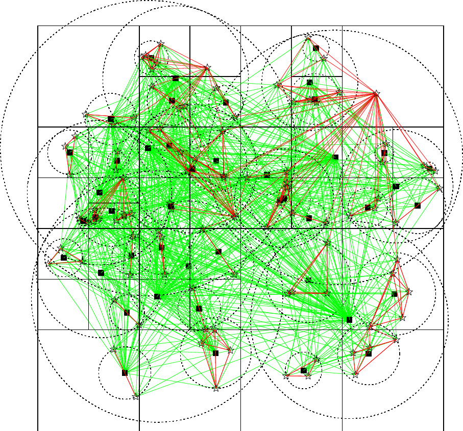
Fig. 5 demonstrates the working of the tree code and compares it graphically to the direct summation approach, by applying both to the task of computing the force for one of 100 particles (left and middle panels). Obviously, the tree code requires much fewer calculations—it is straightforward to show that the number of force computations per particle scales like the depth of the tree, i.e. $\ln N$ , such that the cost of computing all $N$ forces is $\mathcal{O}(N\ln N)$ .

The fast multipole method

(FMM) also works with localised particle groups and for stellar systems is best implemented using a tree structure (139, 140), although the original proposal used a fixed grid (141). In addition to expanding the Greens function $\phi(\vec{x}_{b}-\vec{x}_{a})$ at the source positions $\vec{x}_{a}$ (as for the tree code), it also expands it at the sink positions $\vec{x}_{b}$ (with $\vec{z}_{\!B}$ the centre of the group $B$ of sink particles, see also the left panel of Fig. 6):

\phi(\vec{x}_{b}-\vec{x}_{a})\approx\sum_{|{\vec{\mathsf{n}}}|\leq p}\,\sum_{|{\vec{\mathsf{m}}}|\leq p-n}\frac{(-1)^{\mathsf{n}}}{{\vec{\mathsf{n}}}!{\vec{\mathsf{m}}}!}\,(\vec{x}_{b}-\vec{z}_{\!B})^{\vec{\mathsf{n}}}\,(\vec{x}_{a}-\vec{z}_{\!A})^{\vec{\mathsf{m}}}\,\vec{\nabla}^{{\vec{\mathsf{n}}}+{\vec{\mathsf{m}}}}\phi(\vec{z}_{\!B}-\vec{z}_{\!A}).

(56)

Inserting this into (51), yields for the potential generated by all particles in $A$ and at any position $\vec{x}_{b}$ within $B$

	$\displaystyle\hat{\Phi}_{A\to B}(\vec{x}_{b})$	$\displaystyle\approx$	$\displaystyle\sum_{\|{\vec{\mathsf{n}}}\|\leq p}\frac{1}{{\vec{\mathsf{n}}}!}(\vec{x}_{b}-\vec{z}_{\!B})^{{\vec{\mathsf{n}}}}F_{{\vec{\mathsf{n}}}}(\vec{z}_{\!B}),$		(57)
	$\displaystyle F_{{\vec{\mathsf{n}}}}(\vec{z}_{\!B})$	$\displaystyle=$	$\displaystyle\sum_{\|{\vec{\mathsf{m}}}\|\leq p-n}M_{{\vec{\mathsf{m}}}}(\vec{z}_{\!A})\,D_{{\vec{\mathsf{n}}}+{\vec{\mathsf{m}}}}(\vec{z}_{\!B}-\vec{z}_{\!A})$		(58)

with the multipole moments $M_{{\vec{\mathsf{m}}}}(\vec{z}_{\!A})$ defined in equation (54). The field tensors $F_{{\vec{\mathsf{n}}}}(\vec{z}_{\!B})$ are the coefficients of the Taylor series (57) for the potential around $\vec{z}_{\!B}$ . This dual expansion ‘at both ends’ of all interactions considerably speeds up the simultaneous computation of gravity for all particles, but brings no advantage over the tree code when computing the force at a single position. The FMM algorithm works these equations backwards, starting with an upward pass (as for the tree code) to compute the multipole moments $M_{{\vec{\mathsf{m}}}}(\vec{z}_{\!A})$ and widths $w_{\!A}$ for all cells.

The second part is the interaction phase, when the field tensors are evaluated for each cell. This is achieved by the following algorithm starting with the root-root interaction¹⁷¹⁷ 17 Here, we describe the falcON algorithm (140), but essentially any multipole-based method which expands the Greens functions both at the source and sink positions and therefore performs cell-cell interactions qualifies as FMM.. If for a mutual cell-cell interaction $\theta(w_{\!A}+w_{\!B})<r=|\vec{z}_{A}-\vec{z}_{B}|$ , then the field tensors for the interactions $A\to B$ and $B\to A$ are computed according to equation (58) and added to $F_{{\vec{\mathsf{n}}}}(\vec{z}_{\!B})$ and $F_{{\vec{\mathsf{n}}}}(\vec{z}_{\!A})$ , respectively. Otherwise, the interaction is split into up to 8 new interactions by opening the bigger (in terms of $w$ ) of the two cells. A cell self-interaction (like the initial root-root interaction) is performed by simple direct summation if the cell contains only a few particles, otherwise it is split into up to 36 new interactions.

Finally, in a down-ward pass the contributions from the parent cells are added to the field-tensors of their daughters after applying the shifting formula

F_{{\vec{\mathsf{n}}}}(\vec{z}+\vec{x})=\sum_{|{\vec{\mathsf{k}}}|\leq p-n}\frac{\vec{x}^{{\vec{\mathsf{k}}}}}{{\vec{\mathsf{k}}}!}\,F_{{\vec{\mathsf{n}}}+{\vec{\mathsf{k}}}}(\vec{z}),

(59)

followed by the evaluation of gravity via equation (57) at the sink positions within leaf cells. The total computational costs of this algorithm are dominated by the interaction phase, which only requires $\mathcal{O}(N)$ interactions for the computation of all $N$ particle forces. This represents a substantial reduction from the $\mathcal{O}(N^{2})$ for direct summation. It is also a factor $\gtrsim 10$ faster than the tree code for typical $N\gtrsim 10^{6}$ .

Some practical considerations

1.

The simple convergence criterion $|\vec{r}|<\theta w$ commonly used with the tree code and the FMM is merely geometric and therefore controls the relative error for each interaction (140)

$\frac{|\delta\vec{\nabla}\Phi_{A\to B}|}{|\vec{\nabla}\Phi_{A\to B}|}\leq\frac{(p+1)\theta^{p}}{(1-\theta)^{2}}.$ (60)

However, usually the forces from small (and hence nearby) cells are smaller than from bigger distant cells such that the absolute force error is dominated by the few interactions with big cells. A better approach is therefore to try to balance the force errors by a non-geometric opening criterion, for example using a mass-dependent opening angle. With this, one can obtain a total cost $<\mathcal{O}(N)$ at fixed approximation error (140).
2.

For the un-softened Greens function $\phi=1/r$ , the multipole expansion is reduced from three to two-dimensional indices when using spherical harmonics. Essentially, this exploits the fact that $D_{{\vec{\mathsf{n}}}+2\hat{{\vec{\mathsf{x}}}}}+D_{{\vec{\mathsf{n}}}+2\hat{{\vec{\mathsf{y}}}}}+D_{{\vec{\mathsf{n}}}+2\hat{{\vec{\mathsf{z}}}}}=0$ for any ${\vec{\mathsf{n}}}$ (as a consequence of $0=\vec{\nabla}^{2}\phi$ ), such that the number of independent terms is reduced from $\binom{p+3}{p}$ to $(p+1)^{2}$ . This reduces the costs for the FMM interaction operation (58) from $\mathcal{O}(p^{6})$ to $\mathcal{O}(p^{4})$ , which may be further reduced to $\mathcal{O}(p^{3})$ (by fast rotation methods, e.g. (142)), $\mathcal{O}(p^{2}\ln p)$ (by fast Fourier methods (143)), or even $\mathcal{O}(p^{2})$ (using plane wave approximations (144)).
3.

Both the distribution of force errors and the total computational costs depend on the opening criterion, the expansion order, and other numerical details. For an optimal choice of these numerical parameters, the computational cost depends non-trivially on the required approximation error. With collisionless $N$ -body codes one usually requires only a modest relative force accuracy of $\sim 10^{-3}$ , in which case low-order techniques are sufficient.
4.

Fig. 7 gives an alternative graphical comparison of direct summation, the tree code, and FMM for the computation of all $N$ forces. With direct summation, each pair-wise interaction is considered only once because the mutual forces satisfy $\vec{F}_{\!\!i\!j}=-\vec{F}_{\!\!j\!i}$ , according to Newton’s third law.

With the tree code, this natural symmetry between sinks and sources is broken: each interaction is one-sided. As a consequence, the full interaction matrix (except for the diagonal) has to be approximated and Newton’s third law is violated, implying the loss of total-momentum conservation.

With the FMM on the other hand, each interaction is mutual, exploiting the natural symmetry of the problem and satisfying Newton’s third law for each particle pair (though the approximated $\vec{F}_{\!\!i\!j}$ is not exactly aligned with the separation vector $\vec{x}_{i}-\vec{x}_{\!j}$ ). Only the upper half of the interaction matrix needs to be approximated. Further away from the diagonal, a single cell-cell interaction (blue box) approximates ever more particle-particle interactions.
5.

From Fig. 7 one can also see that for the tree code the workload can be easily split between many processors. This is more difficult with direct summation or the FMM. For example, when distributing the particles amongst processors, it is not obvious which computes the forces between particles (or cells) residing on different processors (but see (Stadel et al., 2009)).

Critique

Apart from the violation of Newton’s third law with the tree code (but not the FMM), the only potential short-coming is a discontinuity of the forces: there are some magic boundaries in space on either side of which a different approximation will be used, depending on the opening criterion. As a consequence, the approximated forces are not conservative across these boundaries and the total energy of the $N$ -body system is not exactly conserved but exhibits some fluctuations, even in the limit of zero time step. Of course, the amplitude of this effect can be reduced by decreasing the opening angle $\theta$ .

It appears that this issue has little if any effect on the validity of the $N$ -body model (there are no obvious differences between results obtained using the tree code and methods which do not suffer from this problem). In principle it should be possible to design a tree code or FMM without this problem by smoothly interpolating between the force approximations on either side of the magic boundaries. The natural adaptivity and efficiency of the tree code and FMM make them versatile and powerful force solvers for general-purpose $N$ -body codes.

3.5.2 Grid-based methods

Instead of solving the integral form (38) or (42) of the Poisson equation, as with direct summation and its approximations, grid-based methods solve its differential form

\vec{\nabla}^{2}\Phi(\vec{x})=4\pi G\rho(\vec{x})

(61)

after discretisation on a grid.

Fast-Fourier-transform-based methods

achieve this in the Fourier domain where the Poisson equation (61) becomes $\vec{k}^{2}\Phi(\vec{k})=4\pi G\rho(\vec{k})$ . The method first estimates the density on the vertices of an equidistant grid by a technique which spreads the mass of each particle across neighbouring cells (see (Hockney & Eastwood, 1988) for details). Next, the Poisson equation is solved, using the fast Fourier transform (FFT), for the value of the potential $\Phi$ on each grid vertex; and finally the potential and force for each particle is found by interpolation between vertices.

This method is fast (the cost for the FFT and the interpolation are $\mathcal{O}(n_{\mathrm{grid}}\ln n_{\mathrm{grid}})$ and $\mathcal{O}(N)$ , respectively), but not effective for inhomogeneous particle distributions typical for most $N$ -body simulations, when in order to resolve the high-density regions $n_{\mathrm{grid}}^{3}\gg N$ is required.

The Fourier approach implicitly assumes a periodic tiling of all space with the computational domain, such that it actually (approximately) solves

\vec{\nabla}^{2}\Phi(\vec{x})=4\pi G\sum_{{\vec{\mathsf{n}}}}\rho(\vec{x}+{\vec{\mathsf{n}}}L).

(62)

This corresponds not to equation (38) but (42), exactly as desired for cosmological $N$ -body simulations of large-scale structure formation. Therefore, FFT-based methods (or hybrid methods using FFT, see below) are predominantly used with such simulations.

The periodic boundary conditions can be avoided either by simply doubling the computational domain in each dimension or better by James’ (James, 1977) method, which subtracts the contributions from the periodic replicas of the computational box via a Fourier technique involving surface charges. Combining this with a set of nested grids of increasing resolution enables an efficient FFT-based force solver for inhomogeneous single stellar systems, such as galaxies (146).

Multi-grid techniques

were pioneered in the west by Brandt (1977) in 1977; they also interpolate the density and potential between grid and particles, but solve the discretised form of the Poisson equation, i.e. a large but sparse matrix equation, using relaxation methods, such as Gauss-Seidel iteration. The basic idea exploits the fact that on a coarser grid relaxation occurs faster because information travels faster. The distribution of errors (the difference between the actual density and that obtained via the discretisation of $\vec{\nabla}^{2}\Phi$ from the current estimate for the potential) is first smoothed on the finest grid by a few Gauss-Seidel iterations. After transferring the problem to a coarser grid, the process is repeated on coarser and coarser grids until, on the coarsest grid convergence is achieved. Then the problem is transferred back to finer and finer grids, each time iterating until convergence.

Since the costs of an iteration shrinks by a factor eight when going to the next coarser grid, the total cost is essentially determined by the costs of a fixed number of iterations on the finest grid, and hence $\mathcal{O}(n_{\mathrm{grid}})$ in theory (148). However, as far as we are aware, in practical applications for $N$ -body simulations, the method is not significantly more efficient than others.

The advantage of this technique over the FFT approach is that the grid does not need to be equidistant, but can be locally adapted according to the particle density. In fact, the structure of such an adaptively refined mesh is identical to that of a shallow oct-tree, as used with the tree-code and FMM.

Critique

Gravitational softening is implicit with grid methods, in contrast to direct summation and its approximations, and depends on the grid size. This means that for adaptive meshes the softening may vary along a particle orbit, depending on the local mesh resolution. Since softening unavoidably leads to a reduction in the estimated binding energy of a particle (§3.4.2), these variations introduce an unphysical fluctuation of particle binding energies. In non-equilibrium simulations, for example of gravitational collapse, this leads to violation of energy conservation and artificial secular evolution. This problem also occurs with individually adapted softening lengths with explicit softening (as with the tree code or FMM), but there a solution is known, see §3.4.4.

With adaptive multi-grid methods, it is natural to use different time steps (within the block-step scheme) for particles living on different refinement levels. Such a scheme can be substantially accelerated by advancing the particles asynchronously: the particles on the coarser grid remain fixed while those on the finer grid move and their gravity is approximated by using the coarser-grid potential as boundary condition. However, such a method is neither Hamiltonian nor time symmetric, potentially resulting in artificial secular evolution (and violation of energy conservation).

3.5.3 Basis function methods

The idea of basis-function methods, pioneered by Clutton-Brock (1972) in 1972 and later dubbed ‘self-consistent field code’ (150), is to expand the mass density into basis functions $\rho_{{\vec{\mathsf{n}}}}(\vec{x})$ with coefficients $C_{{\vec{\mathsf{n}}}}$

\hat{\rho}(\vec{x})=\sum_{{\vec{\mathsf{n}}}}C_{{\vec{\mathsf{n}}}}\,\rho_{{\vec{\mathsf{n}}}}(\vec{x}),

(63)

where ${\vec{\mathsf{n}}}=(n,l,m)$ is a three-dimensional set of indices, and estimate the potential as

\hat{\Phi}(\vec{x})=-G\sum_{{\vec{\mathsf{n}}}}C_{{\vec{\mathsf{n}}}}\,\psi_{{\vec{\mathsf{n}}}}(\vec{x}),

(64)

where $4\pi\rho_{{\vec{\mathsf{n}}}}(\vec{x})=-\vec{\nabla}^{2}\psi_{{\vec{\mathsf{n}}}}(\vec{x})$ . Usually, the sets of basis functions used are complete and bi-orthogonal, i.e. satisfy

$\displaystyle\delta_{{\vec{\mathsf{n}}}{\vec{\mathsf{n}}}^{\prime}}$	$\displaystyle=$	$\displaystyle\int\!\mathrm{d}\vec{x}\,\rho_{{\vec{\mathsf{n}}}}(\vec{x})\,\psi_{{\vec{\mathsf{n}}}^{\prime}}(\vec{x}),$	(65)
$\displaystyle\delta(\vec{x}-\vec{x}^{\prime})$	$\displaystyle=$	$\displaystyle\sum_{{\vec{\mathsf{n}}}}\rho_{{\vec{\mathsf{n}}}}(\vec{x})\,\rho_{{\vec{\mathsf{n}}}}(\vec{x}^{\prime}),$	(66)
$\displaystyle\frac{1}{\|\vec{x}-\vec{x}^{\prime}\|}$	$\displaystyle=$	$\displaystyle\sum_{{\vec{\mathsf{n}}}}\psi_{{\vec{\mathsf{n}}}}(\vec{x})\,\psi_{{\vec{\mathsf{n}}}}(\vec{x}^{\prime}),$	(67)

where the integral is over all space and the sums include all terms $|{\vec{\mathsf{n}}}|\to\infty$ . Applying the bi-orthogonality relation (65) to the density estimate (63) gives $C_{{\vec{\mathsf{n}}}}=\int\!\mathrm{d}\vec{x}\,\hat{\rho}(\vec{x})\,\psi_{{\vec{\mathsf{n}}}}(\vec{x})$ , which upon inserting of the Monte-Carlo estimator for the mass density (equation 40 with $g$ a delta-spike) yields

C_{{\vec{\mathsf{n}}}}=\sum_{i}\mu_{i}\,\psi_{{\vec{\mathsf{n}}}}(\vec{x}_{i}).

(68)

Thus, the basis-function force solver first calculates the coefficients $C_{{\vec{\mathsf{n}}}}$ via equation (68) and subsequently computes potential and force at any position via equation (64) and its derivative. Since both of these operations are trivially split between multiple processes and require minimal communication, this method is ideal for computational parallelism.

Of course, in practice one has to truncate the expansion at some finite order ${\vec{\mathsf{n}}}_{\max}$ . Ideally, the error made by this truncation is small, such that the signal in the neglected coefficients $C_{{\vec{\mathsf{n}}}>{\vec{\mathsf{n}}}_{\max}}$ is negligible. This is usually achieved by choosing the parameters of a given basis-function set such that $\rho_{{\vec{\mathsf{0}}}}$ already closely matches the system modelled and higher-order terms merely describe deviations. A more systematic approach is to design the basis functions to match the system at hand (151) but also to truncate the expansion smoothly according to the estimated signal-to-noise in the neglected coefficients (152).

Critique

Of course, the basis-function approach is not suitable for modelling wildly dynamic situations, such as galaxy mergers, but only for near-equilibrium dynamics, when the stellar system deviates only slightly from the smooth zeroth-order basis function. An advantage of the method is the effective softening, which usually is small in high-density regions where the the basis functions vary mostly. Unlike Greens-function softening, the method does not bias the force of a density cusp ( $\rho\propto r^{-\gamma}$ ) if the basis functions contain the same power-law cusp and the $N$ -body system is centred on the origin of the expansion. In fact, off-centring is a significant problem with this method.

It has been argued that the basis-function method is ideally suited for such near-equilibrium systems, because the computational cost scales linear with $N$ . However, this view is too simplistic, since it is futile to increase $N$ but not also the force resolution, i.e. ${\vec{\mathsf{n}}}_{\max}$ . Simple arguments based on equivalence to Greens-function softening suggest that the optimum resolution for given $N$ requires an increase of ${\vec{\mathsf{n}}}_{\max}$ such that the overall computational cost scale like $\mathcal{O}(N^{2})$ , as for straightforward direct summation (131).

One may hope to alleviate this problem by a continually adapting the lowest-order basis function (151) such that ${\vec{\mathsf{n}}}_{\max}$ can be kept low. However, this approach changes the approximated Greens function

\phi(\vec{x}-\vec{x}^{\prime})=\sum^{{\vec{\mathsf{n}}}_{\max}}_{{\vec{\mathsf{n}}}}\psi_{{\vec{\mathsf{n}}}}(\vec{x})\,\psi_{{\vec{\mathsf{n}}}}(\vec{x}^{\prime})

(69)

during the simulation and therefore introduces an artificial time dependence into the approximate Hamiltonian. At best, this only destroys energy conservation, but more likely has other adverse effects which are less obvious to identify.

The basis-function method may be most useful for simulations with constrained symmetry. For example, enforcing spherical symmetry simply amounts to setting $C_{nlm}\propto\delta_{l0}\delta_{m0}$ when using a basis based on spherical-harmonics. This reduces the computational costs substantially, even when including many radial basis functions, thus enabling extremely fast spherically symmetric simulations with large $N$ . The basis-function method is certainly very useful as force solver for other purposes, for example to approximate the density and/or potential of an external system or to model the potential in perturbation analyses.

3.5.4 Hybrid methods

The advantages and disadvantages of the various force solvers naturally lead to the concept of hybrid methods, to avoid the respective disadvantages. Most relevant in this context is presumably the usage of FFT-based methods to obtain periodic boundary conditions, which are desired in cosmological simulations. The disadvantage of the FFT-based method (also called ‘PM’ particle-mesh) is the lack of resolution and adaptivity on small scales. In the 1980s, the early days of cosmological simulations, the combination of PM with direct summation (‘PP’: particle-particle) for the computation of the near-neighbour force deficit (the difference between the average FFT force and that for the desired softening length) enjoyed some popularity as ‘P³M’ codes (153). Later, this approach has been improved by replacing direct summation with a tree code (‘TreePM’ (154)), but we are not aware of the obvious FMM-PM combination. Combinations of the multi-grid method with the FFT are straightforward (the FFT is used as force solver on the coarsest grid (155)).

Other hybrid methods combine the basis-function approach in a subset of the spatial dimensions with a grid in the remaining, for example using spherical harmonics with a radial grid (156, 157).

3.6 Recent numerical developments and challenges

Collisionless $N$ -body simulations have benefitted enormously from the incredible increase in computer power, in particular as the computational costs only increase like $N\ln N$ (for the tree code and grid methods). This combined with massive parallelisation on many thousand cores has allowed very large $N$ simulations. A further increase by a factor $\sim 10$ should be possible just by using the FMM as force solver (though implementing the FMM efficiently in parallel is challenging). Another welcome numerical advancement would be better time-stepping methods (see the discussion at the end of §2.3.3).

However, the main challenge of contemporary applications of collisionless $N$ -body methods lie not in the method, but in the astrophysics it misses out: any non-gravitational interaction. Baryonic matter contributes only 16% of all matter on large scales (116) and inter-stellar gas contributes only little to the mass of individual galaxies (in the Milky Way the mass ratio between gas and stars is about 1:9). However, the gas not only interacts gravitationally (with all other matter), but can directly dissipate (and absorb) energy in form of radiation, and therefore behaves fundamentally differently from point-mass particles.

One big challenge of contemporary astrophysics is to model the formation of galaxies ab initio. To this end, many complex astrophysical processes and phenomena must be modelled, such as the multi-phase nature of the gas, its condensation to stars and active galactic nuclei (AGN), and their feedback (via winds and radiation) onto the gas (all these process may be summarised as ‘baryon physics’). While hydrodynamics is comparatively straightforward to add to the method, e.g. via smoothed particle hydrodynamics (134), most of the baryonic physics is not. This is because these processes are themselves not properly understood and can only be modelled via parametric ‘sub-resolution’ models. For example, a gas particle is turned into a star particle according to some parametric model of our current understanding of the star formation process. While substantial progress has been made, the challenges are still formidable, not only because of our limited astrophysical understanding of the baryon physics, but also since much higher numerical resolution may be required for convergence than with simple gravity-only $N$ -body experiments.

3.7 Past, recent, and future astrophysical modelling

As in §2.7, we provide a very brief summary of selected (by personal opinion) highlights of astrophysical results based on collisionless $N$ -body simulations (apology to anybody who feels missed-out).

One of the earliest results was the modelling by 158 in 1972 [158, see also 159; 3]¹⁸¹⁸ 18 Sadly, this excellent work is only little-known (63 citations), largely because publishing in the west was extremely difficult for Soviet scientists during the cold-war era. The later study by Toomre & Toomre (ApJ 178, 623) with essentially the same simulation set-up but only $N=120$ (compared to $N=2000$ ) is much more widely known (over 1700 citations). of tidal interactions of rotationally supported disc galaxies, demonstrating a large variety of observed phenomena, such as tidal arms and bridges. Simulations of galaxy interactions could explain many other observed phenomena such as shells, ripples, and other ‘fine structure’ (160, 161, 162, 163), as well as ring galaxies (164). Also, the merger origin of elliptical galaxies received strong support from $N$ -body simulations (165, 166).

The bar instability of isolated disc galaxies was discovered in the first simulations of such systems (167, 168), providing a natural explanation of the high frequency of barred galaxies. More recent simulations suggest a close connection between the dynamics of bars and outer rings (169) and demonstrate the importance of a dark-matter halo as an angular-momentum absorber (170, 171). The buckling instability of bars was first seen in $N$ -body simulations (172), though the identification of ‘boxy’ or ‘peanut-shaped’ bulges as side-on bars was only made later. Simulations of disc galaxies also showed spontaneous formation of transient and/or long-lived spiral features (173), which prompted the theoretical model of swing-amplification by Toomre & Zang (174).

‘Cosmological’ simulations based on cold dark-matter match the observed large-scale structure of the universe (175, 176), while hot (e.g. neutrino) dark-matter is ruled out (177). The dark-matter haloes formed in such simulations possess a universal density profile (21, 178), which varies between $\rho\propto r^{-1}$ at $r\to 0$ and $\rho\propto r^{-3}$ to $r^{-4}$ at large radii, and triaxial shapes (21, 179). This is now observationally confirmed on galaxy cluster scales (180, 181, 182). Finally, such simulations predict a wealth of substructure that should be present orbiting the Milky Way, and in the Local Group that is not (yet) observed (183, 184).

Confronting such predictions, as well as those of almost all applications of collisionless $N$ -body simulations, with observations requires an extension of the method to include baryonic physics (see §3.6). The goal for the coming decades will be realistic simulations of galaxy formation and evolution, which will allow us to test both our current cosmological model, and galaxy formation theories.

4 Validation

A very important issue with $N$ -body techniques is the validation of the numerical method in general and for the specific purpose in particular. While a 100% validation is never possible, there are several powerful validation techniques available. In particular for collisionless $N$ -body techniques, every project requires a validation to ensure that the numerical method (which includes the values of numerical parameters such as $N$ ) guarantees the desired numerical accuracy, thus avoiding systematic errors driven by numerical artifacts.

Validation of the method

Before even considering the application of a certain $N$ -body program (collisional or collisionless) for a particular modelling purpose, the values of numerical parameters (controlling time step, force approximation, etc.) required for correctness must be established. This can be done in two ways: first by simulating simple but non-trivial situations for which the correct outcome is known from other means (such a perturbation analysis or, in the case of collisional $N$ -body code by using any of the alternative methods of §2.6); and second (for collisionless $N$ -body methods) by re-simulating a certain situation with ever better numerical accuracy, which should converge to a (hopefully correct) answer.

Validation by Monitoring

One of the most straightforward validation requirements is the actual numerical conservation of total energy, momentum, and angular momentum. While with a finite time step energy conservation can never be fully achieved, a relative energy conservation to 3-4 digits is usually considered sufficient in practice for collisionless $N$ -body techniques, while for collisional methods 5-6 digits appear to be the norm. A systematic trend of energy hints at an artificial secular evolution and is much more problematic than mere fluctuations. The same applies to momentum and angular momentum.

In order to monitor whether gravitational softening introduces significant bias (if for instance many particles overlap within the softening length), one can compare the virial $W$ and the potential energy $V$ , defined as

W=\sum_{i}\mu_{i}\;\vec{x}_{i}\cdot\vec{\nabla}\left[\hat{\Phi}_{\mathrm{self}}(\vec{x}_{i})+\Phi_{\mathrm{ext}}(\vec{x}_{i})\right],\hskip 20.00003ptV=\sum_{i}\mu_{i}\,\left[\tfrac{1}{2}\hat{\Phi}_{\mathrm{self}}(\vec{x}_{i})+\Phi_{\mathrm{ext}}(\vec{x}_{i})\right]

(70)

with $\hat{\Phi}_{\mathrm{self}}$ and $\Phi_{\mathrm{ext}}$ denoting, respectively, the (approximated and softened) $N$ -body potential and any external potential. For pure Newtonian gravity (unsoftened), one has $W=V$ and deviations from this equality are indicative of the global importance of the gravity reduction due to softening.

Validation by simulation

When the effect of some particular perturbation is to be modelled, for example of an infalling satellite, it is important to ensure that, at the resolution at which the simulation results will be interpreted, a control simulation without the perturbation behaves as expected. Sometimes, this may not be sufficient, for example when the perturber gives rise to additional astrophysical effects not present in and hence not scrutinised by the control simulation. In such a situation one must employ convergence tests: an equivalent simulation at significantly higher resolution should give consistent results. Even this may fail when the simulations converge to the wrong answer.

Validation by comparison

The only way to to shield against this problem is to re-simulate with a completely different $N$ -body method. For example, various $N$ -body tests have been done within the ESF-funded astro-sim project (http://www.astrosim.net/code). With collisionless $N$ -body methods this is often the only reliable validation technique, since there are hardly any non-linear problems with solutions known from other methods (against which one could compare). Such projects are important and have demonstrated that cosmological codes now agree at the 10% level for important metrics (185). This is excellent progress, but not good enough for next generation cosmological probes like Euclid (http://sci.esa.int/euclid).

Validation and interpretation

Simulation results, in particular when unexpected, should never be trusted at face value, but an effort must be made to understand them in astrophysical terms. This is very often non-trivial, because the highly non-linear and complex dynamics is not compatible with any simplifying assumptions that would allow insight by means of approximate analytical models. However, unlike the situation with real stellar systems and galaxies, the $N$ -body model can be analysed (“observed”) in full six-dimensional phase-space allowing a much better handle on the dynamical processes than nature itself. Contemporary analysis techniques for $N$ -body data are still somewhat immature, but their discussion beyond the scope of this paper.

5 Conclusion

We have reviewed some of the latest numerical techniques for modelling collisional and collisionless $N$ -body systems. Our focus throughout has been on purely gravitational $N$ -body simulations, with a view to presenting the key numerical algorithms. Over the past $\sim 50$ years of $N$ -body calculations, the field has undergone dramatic changes. Improved software algorithms, specialised hardware, and efficient parallel programming have meant that $N$ has kept pace with Moore’s Law, nearly doubling every two years. This has allowed us to simulate the most massive star clusters, galaxies, and the Universe as a whole with increasing precision.

It is clear that our modelling of gravity is in good shape. Different codes and techniques give converged results, while both collisional and collisionless simulations continue to push to larger $N$ . However, the coming challenge will be building believable models of baryonic processes in the Universe. This is beyond the scope of this short review, but is the key challenge for future $N$ -body simulations on all scales.

References

Binney & Tremaine (2008) J.J. Binney, S. Tremaine, Galactic dynamics. 2nd ed (Princeton University Press, Princeton 2008)
White (1976) S.D.M. White, MNRAS 174, 19 (1976)
Holmberg (1941) E. Holmberg, ApJ 94, 385 (1941)
von Hoerner (1960) S. von Hoerner, Zeitschrift für Astrophysik 50, 184 (1960)
Aarseth (1963) S.J. Aarseth, MNRAS 126, 223 (1963)
Harfst et al. (2007) S. Harfst, A. Gualandris, D. Merritt, R. Spurzem, S.F. Portegies Zwart, P. Berczik, New Astronomy 12, 357 (2007)
Springel et al. (2005) V. Springel, S.D.M. White, A. Jenkins, C.S. Frenk, N. Yoshida, L. Gao, J. Navarro, R. Thacker, D. Croton, J. Helly, et al., Nature 435, 629 (2005)
Teyssier et al. (2009) R. Teyssier, S. Pires, S. Prunet, D. Aubert, C. Pichon, A. Amara, K. Benabed, S. Colombi, A. Refregier, J. Starck, A&A 497, 335 (2009)
Stadel et al. (2009) J. Stadel, D. Potter, B. Moore, J. Diemand, P. Madau, M. Zemp, M. Kuhlen, V. Quilis, MNRAS 398, L21 (2009)
Iliev et al. (2011) I.T. Iliev, B. Moore, S. Gottlöber, G. Yepes, Y. Hoffman, G. Mellema, MNRAS tmp, 296, arXiv:1005.3139 (2011).
Terlevich (1980) E. Terlevich, in Star Clusters, edited by J.E. Hesser (IAU Symposium 85, 1980)
Inagaki (1986) S. Inagaki, Pub. Astron. Soc. Japan 38, 853 (1986)
Aarseth & Heggie (1993) S.J. Aarseth, D.C. Heggie, in The Globular Cluster-Galaxy Connection, edited by G.H. Smith & J.P. Brodie (Astronomical Society of the Pacific Conference Series 48, 1993)
Spurzem & Aarseth (1996) R. Spurzem, S.J. Aarseth, MNRAS 282, 19 (1996)
Makino (1996) J. Makino, ApJ 471, 796 (1996)
Baumgardt & Makino (2003) H. Baumgardt, J. Makino, MNRAS 340, 227 (2003)
Hut (2010) P. Hut, New Astronomy Review 54, 163 (2010)
(18) P.J.E. Peebles, AJ 75, 13 (1970)
(19) G. Efstathiou, J.W. Eastwood, MNRAS 194, 503 (1981)
(20) C.S. Frenk, S.D.M. White, G. Efstathiou, M. Davis, Nature 317, 595 (1985)
(21) J. Dubinski, R.G. Carlberg, ApJ 378, 496 (1991)
(22) B. Moore, F. Governato, T. Quinn, J. Stadel, G. Lake, ApJ 499, L5 (1998)
(23) S. Ghigna, B. Moore, F. Governato, G. Lake, T. Quinn, J. Stadel, ApJ 544, 616 (2000)
(24) V. Springel, J. Wang, M. Vogelsberger M., A. Ludlow, A. Jenkins, A. Helmi, J.F. Navarro, C.S. Frenk, S.D.M. White, MNRAS 391, 1685 (2008)
Aarseth (2003) S.J. Aarseth, Gravitational N-Body Simulations (Cambridge University Press, Cambridge 2003)
Heggie & Hut (2003) D.C. Heggie, P. Hut, The Gravitational Million-Body Problem: A Multidisciplinary Approach to Star Cluster Dynamics (Cambridge University Press, Cambridge 2003)
Hockney & Eastwood (1988) R.W. Hockney, J.W. Eastwood, Computer simulation using particles, (Hilger, Bristol 1988)
Trenti & Hut (2008) M. Trenti. P. Hut, scholarpedia http://www.scholarpedia.org/article/N-body_simulations (arXiv:0806.3950 2008)
(29) V.A. Antonov, Solution of the problem of stability of stellar system Emden’s density law and the spherical distribution of velocities (Vestnik Leningradskogo Universiteta, Leningrad 1962)
(30) D. Lynden-Bell, R. Wood, MNRAS 138, 495 (1968)
(31) L. Spitzer, Dynamical evolution of globular clusters (Princeton University Press, Princeton 1987)
(32) H. Baumgardt, D.C. Heggie, P. Hut, J. Makino, MNRAS 341, 247 (2003)
(33) D.C. Heggie, MNRAS 173, 729 (1975)
(34) J.G. Hills, AJ 80, 809 (1975)
(35) S.J. Aarseth, J.G. Hills, A&A 21, 255 (1972)
(36) J.M. Fregeau, M.A. Gürkan, K.J. Joshi, F.A. Rasio, ApJ 593, 772 (2003)
(37) D.C. Heggie, M. Trenti, P. Hut, MNRAS 368, 677 (2006)
(38) C.D. Bailyn, ARA&A 33, 133 (1995)
(39) H.B. Perets, D.C. Fabrycky, ApJ 697, 1048 (2009)
(40) B. Lanzoni, N. Sanna, F.R. Ferraro, E. Valenti, G. Beccari, R.P. Schiavon, R.T. Rood, M. Mapelli, S. Sigurdsson, ApJ 663, 1040 (2007)
(41) A. King, ApJ 732, L28 (2011)
Aarseth (2007) S.J. Aarseth, MNRAS 378, 285 (2007)
(43) S. Harfst, A. Gualandris, D. Merritt, S. Mikkola, MNRAS 389, 2 (2008)
(44) E.H. Morgan, R.A. Remillard, M.R. Garcia, ApJ 324, 851 (1988)
(45) A. Ahmad, L. Cohen, J. Comp. Phys. 12, 389 (1973)
Nitadori & Makino (2008) K. Nitadori, J. Makino, New Astronomy 13, 498 (2008)
(47) H. Yoshida, Celestial Mechanichs and Dynamical Astronomy 56, 27 (1993)
(48) Q. Sheng, IMA J. Num. Analysis 9, 199 (1989)
(49) M. Suzuki, J. Math. Phys. 32, 400 (1991)
(50) B. Leimkuhler, S. Reich, Simulating Hamiltonian Dynamics, (Cambridge University Press, Cambridge 2005)
Chin & Chen (2005) S. Chin, C. Chen, Celestial Mechanichs and Dynamical Astronomy 91, 301 (2005)
(52) G.D. Quinlan, S. Tremaine, AJ 100, 1694 (1990)
(53) P. Hut, J. Makino, S.L.W. McMillan, ApJ 443, L93 (1995)
(54) T. Holder, B. Leimkuhler, S. Reich, Applied Numerical Mathematics 39, 367 (1999)
(55) E. Kokubo, K. Yoshinaga, J. Makino, MNRAS 297, 1067 (1998)
(56) J. Makino, Pub. Astron. Soc. Japan 43, 859 (1991)
Makino et al. (2006) J. Makino, P. Hut, M. Kaplan, H. Saygın, New Astronomy 12, 124 (2006)
Zemp et al. (2007) M. Zemp, J. Stadel, B. Moore, C.M. Carollo, MNRAS 376, 273 (2007)
(59) J. Makino, ApJ 369, 200 (1991)
(60) P. Kustaanheimo, A. Schinzel, H. Davenport, E. Stiefel, Journal für die reine und angewandte Mathematik 218, 204 (1965)
(61) H. Yoshida, Celestial Mechanics 28, 239 (1982)
(62) S.J. Aarseth, K. Zare, Celestial Mechanics 10, 185 (1974)
(63) D.C. Heggie, Celestial Mechanics 10, 217 (1974)
(64) S. Mikkola, S.J. Aarseth, Celestial Mechanichs and Dynamical Astronomy 47, 375 (1990)
(65) S. Mikkola, S.J. Aarseth, Celestial Mechanichs and Dynamical Astronomy 57, 439 (1993)
(66) S. Mikkola, S.J. Aarseth, Celestial Mechanichs and Dynamical Astronomy 84, 343 (2002)
Ito et al. (1990) T. Ito, J. Makino, T. Ebisuzaki, D. Sugimoto, Computer Physics Communications 60, 187 (1990)
(68) J. Makino, T. Fukushige, M. Koga, K. Namura, Pub. Astron. Soc. Japan 55, 1163 (2003)
(69) T. Fukushige, J. Makino, A. Kawai, Pub. Astron. Soc. Japan 57, 1009 (2005)
(70) J. Makino, in Dynamical Evolution of Dense Stellar Systems, edited by E. Vesperini, M. Giersz, & A. Sills (IAU Symposium 246, 2008)
(71) E. Gaburov, S. Harfst, S.F. Portegies Zwart, New Astronomy 14, 630 (2009)
Cohn (1979) H. Cohn, ApJ 234, 1036 (1979)
(73) K. Takahashi, Pub. Astron. Soc. Japan 47, 561 (1995)
Hénon (1971) M. Hénon, Ap&SS 13, 284 (1971)
(75) M. Freitag, W. Benz, A&A 375, 711 (2001)
(76) R.B. Larson, MNRAS 147, 323 (1970)
(77) R. Spurzem, K. Takahashi, MNRAS 272, 772 (1995)
(78) D.C. Heggie, M. Giersz, R. Spurzem, K. Takahashi, Highlights of Astronomy 11, 591 (1998)
(79) E. Kim, I. Yoon, H.M. Lee, R. Spurzem, MNRAS 383, 2 (2008)
Balescu (1960) R. Balescu, Physics of Fluids 3, 52 (1960)
Lenard (1960) A. Lenard, Annals of Physics 10, 390 (1960)
(82) J. Heyvaerts, MNRAS 407, 355 (2010)
(83) M. Giersz, D.C. Heggie, MNRAS 268, 257 (1994)
(84) D. Sugimoto, E. Bettwieser, MNRAS 204, 19P (1983)
(85) S.L.W. McMillan, P. Hut, J. Makino, ApJ 362, 522 (1990)
(86) A. Tanikawa, T. Fukushige, Pub. Astron. Soc. Japan 61, 721 (2009)
(87) W.E. Harris, AJ 112, 1487 (1996)
(88) C.D. Bailyn, R.K. Jain, P. Coppi, J.A. Orosz, ApJ 499, 367 (1998)
(89) J. Magorrian, S. Tremaine, D. Richstone, R. Bender, G. Bower, A. Dressler, S.M. Faber, K. Gebhardt, R. Green, C. Grillmair, J. Kormendy, T. Lauer, AJ 115, 2285 (1998)
(90) J.E. Greene, C.Y. Peng, M. Kim, C. Kuo, J.A. Braatz, C.M. Violette Impellizzeri, J.J. Condon, K.Y. Lo, C. Henkel, M.J. Reid, ApJ 721, 26 (2010)
(91) P. Madau, M.J. Rees, ApJ 551, L27 (2001)
(92) M. Volonteri, F. Haardt, P. Madau, ApJ 582, 559 (2003)
(93) S.F. Portegies Zwart, S.L.W. McMillan, ApJ 576, 899 (2002)
(94) S.F. Portegies Zwart, H. Baumgardt, P. Hut, J. Makino, S.L.W. McMillan, Nature 428, 724 (2004)
(95) K. Gebhardt, R.M. Rich, L.C. Ho, ApJ 578, L41 (2002)
(96) K. Gebhardt, R.M. Rich, L.C. Ho, ApJ 634, 1093 (2005)
(97) H. Baumgardt, J. Makino, P. Hut, S.L.W. McMillan, S.F. Portegies Zwart, ApJ 589, L25 (2003)
(98) H. Baumgardt, J. Makino, P. Hut, ApJ 620, 238 (2005)
(99) A.C. Phillips, The Physics of Stars, 2nd Edition, (Wiley, 1999)
(100) R.P. Church, J. Dischler, M.B. Davies, C.A. Tout, T. Adams, M.E. Beer, MNRAS 395, 1127 (2009)
(101) C. Lajoie, A. Sills, ApJ 726, 66 (2011)
(102) A. Sills, J.C. Lombardi, Jr., C.D. Bailyn, P. Demarque, F.A. Rasio, S.L. Shapiro, ApJ 487, 290 (1997)
(103) I.A. Bonnell, M.R. Bate, H. Zinnecker, MNRAS 298, 93 (1998)
(104) H. Baumgardt, R.S. Klessen, MNRAS tmp, 321, arXiv:1009.1189 (2011)
(105) D.J. Faulkner, K.C. Freeman, ApJ 211, 77 (1977)
(106) W. Priestley, M. Ruffert, M. Salaris, MNRAS 411, 1935 (2011)
Terlevich (1987) E. Terlevich, MNRAS 224, 193 (1987)
(108) S.F. Portegies Zwart, S.L.W. McMillan, P. Hut, J. Makino, MNRAS 321, 199 (2001)
(109) H. Baumgardt, P. Hut, J. Makino, S.L.W. McMillan, S.F. Portegies Zwart, ApJ 582, L21 (2003)
(110) J.R. Hurley, O.R. Pols, S.J. Aarseth, C.A. Tout, MNRAS 363, 293 (2005)
(111) R.P. Church, C.A. Tout, J.R. Hurley, Pub. Astron. Soc. Australia 26, 92 (2009)
(112) P. Hut, M.M. Shara, S.J. Aarseth, R.S. Klessen, J.C. Lombardi, Jr., J. Makino, S. McMillan, O.R. Pols, P.J. Teuben, R.F. Webbink, New Astronomy 8, 337 (2003)
(113) A. Sills, S. Deiters, P. Eggleton, M. Freitag, M. Giersz, D.C. Heggie, J. Hurley, P. Hut, N. Ivanova, R.S. Klessen, et al., New Astronomy 8, 605 (2003)
(114) M.B. Davies, P. Amaro-Seoane, C. Bassa, J. Dale, F. de Angeli, M. Freitag, P. Kroupa, D. Mackey, M.C. Miller, S.F. Portegies Zwart, New Astronomy 12, 201 (2006)
(115) R. Spurzem, in JENAM-2007, “Our Non-Stable Universe” (2007)
(116) E. Komatsu, K.M. Smith, J. Dunkley, C. L. Bennett, B. Gold, G. Hinshaw, N. Jarosik, D. Larson, M.R. Nolta, L. Page, et al., ApJS 192, 18 (2011)
Cooperstock et al. (1998) F.I. Cooperstock, V. Faraoni, D.N. Vollick, ApJ 503, 61 (1998)
(118) V.F. Mukhanov, L.R.W. Abramo, R.H. Brandenberger, Physical Review Letters 78, 1624 (1997)
(119) T. Buchert, M. Kerscher, C. Sicka, Physical Review D 62, 043525 (2000)
(120) A. Ishibashi, R.M. Wald, Classial and Quantum Gravity 23, 235 (2006)
(121) A. Enea Romano, P. Chen, arXiv:1104.0730 (2011)
(122) P.J.E. Peebles, The large-scale structure of the universe, (Princeton University Press, 1980)
(123) V. Springel, MNRAS 364, 1105 (2005)
Ewald (1921) P.P. Ewald, Annalen der Physik 369, 253 (1921)
Hernquist et al. (1991) L. Hernquist, F.R. Bouchet, Y. Suto, ApJS 75, 231 (1991)
(126) R. Klessen, MNRAS 292, 11 (1997)
(127) B.W. Silverman, Density estimation for statistics and data analysis, (Chapman & Hall, London, 1986)
Plummer (1911) H.C. Plummer, MNRAS 71, 460 (1911)
(129) S.D.M. White, MNRAS 189, 831 (1979)
(130) C. Theis, A&A 330, 1180 (1998)
(131) W. Dehnen, MNRAS 324, 273 (2001)
Power et al. (2003) C. Power, J.F. Navarro, A. Jenkins, C.S. Frenk, S.D.M. White, V. Springel, J. Stadel, T. Quinn, MNRAS 338, 14 (2003)
Saitoh & Makino (2010) T.R. Saitoh, J. Makino, arXiv:1005.1752 (2010)
(134) D.J. Price, J. Comp. Phys., in press (arXiv:1012.1885, 2011)
(135) L. Cullen, W. Dehnen, MNRAS 408, 669 (2010)
Price & Monaghan (2007) D.J. Price, J.J. Monaghan, MNRAS 374, 1347 (2007)
Barnes & Hut (1986) J.E. Barnes, P. Hut, Nature 324, 446 (1986)
(138) J.K. Salmon, M.S. Warren, J. Comp. Phys. 111, 136 (1994)
(139) W. Dehnen, ApJ 536, L39 (2000)
(140) W. Dehnen, J. Comp. Phys. 179, 27 (2002)
(141) L. Greengard, V. Rokhlin, J. Comp. Phys. 73, 325 (1987)
(142) D. Pinchon, P.E. Hoggan, J. Phys. A: Math. Theory 40, 1597 (2007)
(143) W.D. Elliott, J.A. Board, Jr., SIAM J. Sci. Comp. 17, 398 (1996)
(144) H. Cheng, L. Greengard, V. Rokhlin, J. Comp. Phys. 155, 468 (1999)
James (1977) R.A. James, J. Comp. Phys. 25, 71 (1977)
(146) J. Magorrian, MNRAS 381, 1663 (2007)
Brandt (1977) A. Brandt, Mathematics of Computation 31, pp. 333 (1977)
(148) U. Trottenberg, C.W. Oosterlee, A. Schüller, Multigrid (Academic Press, 2001)
Clutton-Brock (1972) M. Clutton-Brock, Ap&SS 16, 101 (1972)
(150) L. Hernquist, J.P. Ostriker, ApJ 386, 375 (1992)
(151) M.D. Weinberg, AJ 117, 629 (1999)
(152) M.D. Weinberg, ApJ 470, 715 (1996)
(153) G. Efstathiou, M. Davis, S.D.M. White, C.S. Frenk, ApJS 57, 241 (1985)
(154) P. Bode, J.P. Ostriker, ApJS 145, 1 (2003)
(155) A.V. Kravtsov, A.A. Klypin, A.M. Khokhlov, ApJS 111, 73 (1997)
(156) T.A. McGlynn, ApJ 281, 13 (1984)
(157) M. Trenti, G. Bertin, T.S. van Albada, A&A 433, 57 (2005)
(158) N.N. Kozlov, R.A. Syunyaev, T.M. Éneev, Soviet Physics Doklady 17, 413 (1972)
(159) T.M. Éneev, N.N. Kozlov, R.A. Sunyaev, A&A 22, 41 (1973)
(160) P.J. Quinn, ApJ 279, 596 (1984)
(161) C. Dupraz, F. Combes, A&A 166, 53 (1986)
(162) L. Hernquist, P.J. Quinn, ApJ 331, 682 (1988)
(163) L. Hernquist, P.J. Quinn, ApJ 342, 1 (1989)
(164) R. Lynds, A. Toomre, ApJ 209, 382 (1976)
(165) J.E. Barnes, ApJ 331, 699 (1988)
(166) J.E. Barnes, Nature 344, 379 (1990)
(167) R.H. Miller, K.H. Prendergast, W.J. Quirk, ApJ 161, 903 (1970)
(168) F. Hohl, ApJ 168, 343 (1971)
(169) E. Athanassoula, M. Romero-Gómez, J.J. Masdemont, MNRAS 394, 67 (2009)
(170) E. Athanassoula, MNRAS 341, 1179 (2003)
(171) J. Dubinski, I. Berentzen, I. Shlosman, ApJ 697, 293 (2009)
(172) F. Combes, R. H. Sanders, A&A 96, 164 (1981)
(173) T. Zang, PhD thesis (Massachusetts Institute of Technology, 1976)
(174) A. Toomre, in Structure and Evolution of Normal Galaxies, edited by S.M. Fall & D. Lynden-Bell (1981)
(175) M. Davis, G. Efstathiou, C.S. Frenk, S.D.M. White, ApJ 292, 371 (1985)
(176) V. Springel, C.S. Frenk, S.D.M. White, Nature 440, 1137 (2006)
(177) S.D.M. White, C.S. Frenk, M. Davis, ApJ 274, L1 (1983)
(178) J.F. Navarro, C.S. Frenk, S.D.M. White, ApJ 462, 563 (1996)
(179) M.S. Warren, P.J. Quinn, J.K. Salmon, W.H. Zurek, ApJ 399, 405 (1992)
(180) P. Saha, J.I. Read, L.L.R. Williams, ApJ 652, L5 (2006)
(181) P. Saha, J.I. Read, ApJ 690, 154 (2009)
(182) K. Umetsu, T. Broadhurst, A. Zitrin, E. Medezinski, D. Coe, M. Postman, arXiv:1105.0444 (2011)
(183) A. Klypin, A.V. Kravtsov, O. Valenzuela, F. Prada, ApJ 522, 82 (1999)
(184) B. Moore, S. Ghigna, F. Governato, G. Lake, T. Quinn, J. Stadel, P. Tozzi, ApJ 524, L19 (1999)
(185) K. Heitmann, Z. Lukić, P. Fasel, S. Habib, M.S. Warren, M. White, J. Ahrens, L. Ankeny, R. Armstrong, B. O’Shea, P.M. Ricker, V. Springel, J. Stadel, H. Trac, Computational Science and Discovery 1, 015003 (2008)

𝑵N-body simulations of gravitational dynamics

Abstract

pacs

1 Introduction

2 N-body methods for collisional systems

2.1 Equations governing collisional stellar systems

2.2 Numerics of collisional N-body simulations

2.3 Time integration

2.3.1 The Leapfrog integrator

2.3.2 Hermite integrators

2.3.3 The choice of time-step

2.3.4 Close encounters and regularisation

2.4 Recent numerical developments

2.5 Critique and numerical alternatives

2.6 Alternatives to N-body simulations

Orbit averaging

Monte-Carlo

Fluid Models

2.7 Past, recent, and future astrophysical modelling

3 N-body methods for collisionless systems

3.1 Equations governing collisionless stellar systems

3.2 Numerics of collisionless N-body simulations

3.3 Cosmological N-body simulations

3.4 Force softening

3.4.1 Softening as a method to suppress close encounters

3.4.2 Softening as optimal force estimation: the choice of the softening kernel

3.4.3 The choice of the softening length

3.4.4 Adaptive individual softening

3.5 Force computation

3.5.1 Approximating direct summation

The tree code

The fast multipole method

Some practical considerations

Critique

3.5.2 Grid-based methods

Fast-Fourier-transform-based methods

Multi-grid techniques

Critique

3.5.3 Basis function methods

Critique

3.5.4 Hybrid methods

3.6 Recent numerical developments and challenges

3.7 Past, recent, and future astrophysical modelling

4 Validation

Validation of the method

Validation by Monitoring

Validation by simulation

Validation by comparison

Validation and interpretation

5 Conclusion

References

$N$ -body simulations of gravitational dynamics