The SDSS-III Baryon Oscillation Spectroscopic Survey:
Quasar Target Selection for Data Release Nine
Abstract
The SDSS-III Baryon Oscillation Spectroscopic Survey (BOSS), a five-year spectroscopic survey of 10,000 deg2, achieved first light in late 2009. One of the key goals of BOSS is to measure the signature of baryon acoustic oscillations in the distribution of Ly absorption from the spectra of a sample of 150,000 quasars. Along with measuring the angular diameter distance at , BOSS will provide the first direct measurement of the expansion rate of the Universe at . One of the biggest challenges in achieving this goal is an efficient target selection algorithm for quasars in the redshift range , where their colors tend to overlap those of the far more numerous stars. During the first year of the BOSS survey, quasar target selection methods were developed and tested to meet the requirement of delivering at least 15 quasars deg-2 in this redshift range, with a goal of 20, out of 40 targets deg-2 allocated to the quasar survey. To achieve these surface densities, the magnitude limit of the quasar targets was set at or . While detection of the BAO signature in the distribution of Ly absorption in quasar spectra does not require a uniform target selection algorithm, many other astrophysical studies do. We have therefore defined a uniformly-selected subsample of 20 targets deg-2, for which the selection efficiency is just over 50% (10 quasars deg-2). This “CORE” subsample will be fixed for Years Two through Five of the survey. For the remaining 20 targets deg-2, we will continue to develop improved selection techniques, including the use of additional data sets beyond the SDSS imaging data. In this paper we describe the evolution and implementation of the BOSS quasar target selection algorithms during the first two years of BOSS operations (through July 2011), in support of the science investigations based on these data, and we analyze the spectra obtained during the first year. During this year, 11,263 new quasars were spectroscopically confirmed by the BOSS, roughly double the number of previously known quasars with . Our current algorithms select an average of 15 quasars deg-2 from 40 targets deg-2 using single-epoch SDSS imaging. Multi-epoch optical data and data at other wavelengths can further improve the efficiency and completeness of BOSS quasar target selection.
Subject headings
surveys - quasars: Lyman- forest, cosmology: classification techniques
I. Introduction
I.1. The Baryon Oscillation Spectroscopic Survey
The current Cosmic Microwave Background (CMB) data are in excellent agreement with the theoretical predictions of a flat cosmological model with cold dark matter which is dominated by dark energy with an equation of state parameter, [49, 51, CDM; ]. Acoustic peaks in the CMB anisotropy power spectrum are generated by cosmological perturbations exciting sound waves in the relativistic plasma of the early universe [97, 71, 11, 12, 41, 63]. The scale of these peaks, which is set by the sound horizon at last scattering [26, 9, 89], can be used as a cosmological standard ruler. These baryon acoustic oscillations (BAO) are present in the distribution of matter at late times as well, and were first measured in the large-scale distribution of galaxies by Eisenstein et al. [25] and Cole et al. [18].
BAO should also be present in the distribution of neutral hydrogen gas in the intergalactic medium, and thus should be observable in the Lyman- forest (LyF) absorption spectra of distant quasars [100, 60, 93, 66, 6, 101, 62]. Measurements of BAO in the LyF would provide the first measurements of cosmic expansion and the angular diameter distance at redshift (other than the CMB itself), a regime not constrained by current data, thus giving important constraints on, and tests of, the standard cosmological model.
The Sloan Digital Sky Survey (York et al. 106) is now in its third phase (SDSS-III; Eisenstein et al. 27), and is carrying out a combination of four interleaved surveys that will continue until the summer of 2014. One of those surveys, the Baryon Oscillation Spectroscopic Survey (BOSS11 1 http://www.sdss3.org/surveys/boss.php) commenced operations in late 2009, and is using essentially all the dark time for SDSS-III. The key goal of the BOSS is to measure the absolute cosmic distance scale and expansion rate to an accuracy of a few percent from the signature of BAO in the distribution of galaxies and neutral hydrogen [85, 84]. This will be achieved by measuring spectroscopic redshifts for million luminous red galaxies and, simultaneously, the LyF towards 150,000 high-redshift quasars22 2 In this paper we will use the language “low” and “high” redshift to indicate objects with and , respectively. The term “mid-” will be used to explicitly refer to quasars with .. Both samples aim to constrain the equation of state of dark energy by measuring the angular diameter distance, , and the Hubble Parameter, , at and 2.5. In addition to the cosmology goals, the unprecedented dataset of 2.5 quasars will enable tests of black hole growth, wind and feedback models and provide insights into the links between galaxy formation, evolution and luminous AGN activity. Using data from the original SDSS quasar survey will also allow studies of spectroscopic variability. BOSS uses the same 2.5m Sloan Foundation telescope [35] that was used in SDSS-I/II, but since BOSS will observe fainter targets, the fiber-fed spectrographs have been significantly upgraded. These upgrades include: new CCDs with improved blue and red response; 1000 instead of 640 optical diameter fibers; higher throughput gratings over a spectral range of 3600–10000Å at a resolution of about 2000, and improved optics.
| Quantity/units | Year | Full |
| One | Survey∗ | |
| Area (deg2) | 880 | 10,200 |
| Target density in NGC (deg-2) | 80 | 50 |
| Target density in SGC (deg-2) | 70 | 40 |
| Total number of Targets / | 133 | 440 |
| Efficiency | 0.26 | 0.40 |
| Number of quasars / | 13.5 | 175 |
I.2. Quasar Target Selection in BOSS
Quasars have colors distinct from those of the much more numerous stars in the five-color photometry of the SDSS [29]. Unobscured quasars have very blue continua, without any breaks redward of the Ly emission line, and so can be distinguished from hot stars which have a strong Balmer break in the color-color diagram (Figure 1). In particular, at , quasars have a UV excess (as measured by ) that distinguishes them from most stars, and they lie well away from the stellar locus at most higher redshifts (but see below). SDSS-I/II targeted quasars for spectroscopy [75] by selecting point sources which lie far from the locus of stars in color-color space (and all extended sources with a strong UV excess), as well as point sources with radio emission from the Faint Radio Sources at Twenty cm (FIRST) survey [7]. The majority of the more than 100,000 quasars spectroscopically observed by SDSS [88] were targeted in this way.
The Ly forest enters the sensitive range of the BOSS spectrographs at , and the number density of quasars falls dramatically at [68, 87, 78], so BOSS quasar target selection is designed to focus on the range . However, at , SDSS quasar colors are very similar to those of A stars and blue horizontal branch stars [29], thus the optimal quasars for studying the Ly forest are the most difficult ones for BOSS to target. Indeed, the SDSS-I/II quasar target selection algorithm deliberately sparse-sampled objects in the region of color space where quasars should lie [75], in an attempt to minimize the contamination by stars.
The BOSS survey requirements are for spectroscopy of 15 or more quasars deg-2 (150,000 quasars over the BOSS footprint of 10,000 deg2; Eisenstein et al. 27). Combining calculations from McDonald & Eisenstein [60] and McQuinn & White [62] with the luminosity function given by Jiang et al. [46], we find that targeting to a magnitude of with perfect completeness will provide a surface density of quasars deg-2. This magnitude limit is approaching the detection limit of SDSS photometry [1], meaning that photometric errors will significantly broaden the stellar locus (Figure 1) and star-galaxy separation will be a factor. Contamination at both the bright and the faint end of the BOSS target range is mainly from metal-poor halo A and F stars, faint lower redshift () quasars, and compact galaxies. To put these requirements into perspective, the final quasar catalog from the original SDSS-I/II quasar survey [88] contained 17,582 objects over 9380 deg2, while the 2dF-SDSS LRG And QSO (2SLAQ) survey [20], which observed to and concentrated on UV-excess objects, contained 1,110 such quasars selected over 192 deg2. The original 2dF QSO redshift survey (2QZ; Croom et al. 21) focused on the redshift range .
These challenges required a new approach to quasar target selection. The first year of the BOSS survey (“Year One”; 2009 September through July 2010) was devoted in part to refining our algorithms for selecting these objects. The resulting sample of quasars at is comparable in size to the SDSS high-redshift quasar sample, and of course reaches much fainter magnitudes with much higher surface density. Thus the new sample itself represents the best test of our selection algorithms, and we modified those algorithms multiple times through the year. Year One included roughly three months of commissioning of the upgraded BOSS spectrographs and instrument control software as well as a steady ramp-up to full efficiency operations, so it includes well under 20% of the anticipated final sample for the five-year BOSS survey. As of April 2011, BOSS is on track to complete its intended 10,000 deg2 of spectroscopic survey area assuming historical weather patterns and continuation of the current observing efficiency.
Motivated by the first science investigations based on Year One data [92, e.g., ], this paper presents the methods and performance of the quasar target selection during this year. In what follows,“Year Two” will refer both to the spectroscopic observations carried out during BOSS’ second year, 2010 August to 2011 July, and the results of the quasar target selection presented in this paper over the entire 10,000 deg2 BOSS footprint; the distinction should be clear from context. Data from spectroscopic observations in Years One and Two will be included in SDSS Data Release Nine (DR933 3 http://www.sdss3.org/surveys/). The final SDSS-III quasar target selection algorithm will appear in a separate paper.
Background quasars have no causal influence on structure in the LyF at the BAO scale44 4 There may however be some measurement bias at the % level for the flux power spectrum, optical depth and the flux probability distribution, due to gravitational lensing effects, [54, see e.g., ].. Hence the sample of quasars we use for LyF cosmological studies may be quite heterogeneous, with the only consequence that the window function of the survey will depend on the distribution of the quasars for which we have spectra. Since the precision of the BAO measurement improves rapidly with the surface density of quasars (at fixed spectroscopic signal-to-noise ratio (S/N)), we have implemented a target selection scheme in BOSS that can maximize the number of quasars found at in any area of the sky, taking advantage of any available information (e.g., auxiliary data). In Year One, we explored a variety of methods, settling on our final target selection algorithms late in the year.
At the same time, in order to use the quasars themselves for statistical studies (such as luminosity functions or clustering analyses), we must also produce a uniformly selected sample, which we refer to hereafter as CORE (§ III.1). However, we changed the definition of the CORE sample several times over Year One, as we tested various algorithms. Therefore, our fully uniform quasar sample will not include data from this first year of the survey. However, statistical studies (luminosity functions, clustering, and so forth) can utilize all five years of BOSS data by including moderate incompleteness corrections for Year One selection relative to the final CORE algorithm (see §VI). We describe the evolution of our algorithms in detail in this paper, concluding with a description of the method we finally adopted. We give the target selection for both Years One and Two, and thus for the DR9, and analyze our performance from spectra obtained in Year One. By the end of Year Two, quasar target selection (QTS) had been performed over the whole 10,000 deg2 BOSS footprint. Data from Year One were gathered over 880 deg2; see Table 1.
This paper is organized as follows. In § II we describe the SDSS photometry on which the target selection algorithms are most heavily based. Section III describes our methods for selecting quasars [79, 105, 48, 13]. These four papers suggest different, but complementary, methods, and we have used a union of these techniques in different combinations through the survey. In Section IV we describe the implementation of these targeting methods through the first year. In Section V, we report on the global properties of the resulting sample, including high- quasar targeting efficiency, from the data gathered during the first year of the BOSS, and we compare the effectiveness of the various methods. In Section VI we discuss the production of a statistical quasar sample. We conclude in Section VII and suggest improvements to BOSS quasar target selection for the remainder (Years Three, Four and Five) of the survey. Appendix A tabulates the logical cuts used on the input imaging data. Appendix B gives more detail about Year One target selection, while Appendix C describes a pre-BOSS pilot survey using the MMT. Appendix D characterizes the redshift completeness of our spectroscopic data.
We assume a cosmological model throughout with , , [49]. All optical magnitudes are quoted in, and based upon, the SDSS approximation to the AB zero-point system [67, 3], while all near-infrared (NIR) magnitudes are based on the Vega system. Throughout the paper, “magnitude” refers to SDSS Point Spread Function (PSF) magnitudes [96].
II. SDSS Photometry
II.1. Imaging Data
BOSS uses the same imaging data as that of the original SDSS-I/II survey, with an extension in the South Galactic Cap (SGC). These data were gathered using a dedicated 2.5 m wide-field telescope [35] to collect light for a camera with 30 2k2k CCDs [34] over five broad bands - ugriz [31]; this camera has imaged 14,555 unique deg2 of the sky, including 7,500 deg2 in the North Galactic Cap (NGC) and 3,100 deg2 in the SGC [5]. The imaging data were taken on dark photometric nights of good seeing [40], and objects were detected and their properties were measured [55, 96] and calibrated photometrically [95, 45, 98, 69], and astrometrically [73].
Padmanabhan et al. [69] present an algorithm which uses overlaps between SDSS imaging scans to photometrically calibrate the SDSS imaging data. BOSS target selection uses data calibrated using this algorithm from the SDSS Data Release Eight (DR8) database [5, Sec. 3.3; ]. The -wide stripe along the celestial equator in the Southern Galactic Cap, commonly referred to as “Stripe 82” was imaged multiple times, with up to 80 epochs at each point along the stripe spanning a 10-year baseline [2]. In Section IV we will discuss how the commissioning phase of BOSS used coadded catalogs in SDSS Stripe 82, generated by averaging the photometric measurements from individual repeat scans; the details are discussed in Appendix A.6 and in Kirkpatrick et al. [48].
Roughly 50% of the SDSS footprint has been imaged more than once [5]; combining the photometric measurements in these overlap regions reduces the flux errors.
Using the imaging data, BOSS quasar target candidates are selected for spectroscopic observation based on their PSF fluxes and colors in SDSS bands. Fluxes that are used for quasar target selection are corrected for Galactic dust extinction according to the maps of Schlegel et al. [86]. All objects classified as point-like (OBJC_TYPE 6) and are brighter than or are passed to the various quasar target selection algorithms. The joint magnitude limit was imposed due to concerns of the LyF moving into the -band at resulting in suppressed flux at redshifts greater than this. In practice, almost all our targets satisfy both these conditions. Throughout this paper, magnitudes use the asinh scale at low flux levels, as described by Lupton et al. [56].
II.2. Photometric Pipeline Flag and Logic Cuts
During processing of the imaging data by the SDSS photometric pipeline, a number of photometric flags are set for each detected object [96]. These are generated by the SDSS photometric pipeline [55], the Resolve algorithm [5], and by photometric calibration [69]. Some of these flags indicate problems with the de-blending of close pairs of objects. Other flags are set due to poor or unreliable photometry, e.g., if an object was saturated due to a bright star’s diffraction spike or an object was too close to the edge of a frame. If these flags are ignored, they can lead to artifacts in the imaging data being selected as quasar targets. Details of these flags are given in Stoughton et al. [96] and have been updated in DR8 [5].
There are four distinct sets of quasars targeted by BOSS: targets selected by a uniform method, targets selected in a non-uniform way, matches to previously known quasars, and matches to objects in the FIRST survey. We refer to these subsets of targets in this paper as CORE, BONUS, KNOWN and FIRST, respectively.
Each of our targeting algorithms has different imaging flag cuts, as well as different flux limits imposed. We refer to these criteria collectively as “logic cuts.” All such cuts are applied using single-epoch data with one exception: color cuts made on FIRST targets use coadded, multi-epoch data wherever these are available. FIRST objects are thus not considered to be part of the CORE statistical sample, unless they independently meet the CORE selection criteria. The logic cuts are described in detail in Appendix A.
III. Methods for BOSS Quasar Target Selection
III.1. Philosophy of CORE and BONUS
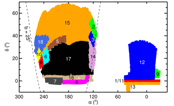
The methods, data and logic flag cuts for BOSS Quasar Target Selection (QTS) are summarized in Fig. 2. During Year One, we carried out QTS and designed spectroscopic plates on areas of 100-300 deg2 at a time. We refer to these areas, within which all the algorithms used in QTS are uniform, as “chunks”. Once QTS was more settled in Year Two, the areas of chunks could be, and sometimes were, more than deg2. For guidance in the following discussion, Chunks 1 through 9, inclusive, constitute Year One, and Chunks 10 through 18, Year Two. Stripe 82 was targeted twice with different targeting algorithms: once in Year One (Chunk 1) and once in Year Two (Chunk 11).
If an object satisfies the selection criteria of one or more of our methods outlined below, bits in the BOSS_TARGET1 target flag are set. Table 2 gives the flag name, the bit value and the short description of the different target selection flags.
| BOSS_TARGET1 flag | bit | Description | Used in Year Two? |
| QSO_COREa | 10 | Restrictive quasar selection | No |
| QSO_BONUSa | 11 | Permissive quasar selection | No |
| QSO_KNOWN_MIDZ | 12 | Known quasar with | Yes |
| QSO_KNOWN_LOHIZb | 13 | Known quasar with | Yes |
| QSO_NNc | 14 | Neural Net | Yes |
| QSO_UKIDSSd | 15 | K-excess targets | No |
| QSO_KDE_COADD | 16 | KDE targets from the Stripe82 coadd | No |
| QSO_LIKE | 17 | Likelihood method | Yes |
| QSO_FIRST_BOSS | 18 | FIRST radio match | Yes |
| QSO_KDE | 19 | Selected by KDE | Yes |
| QSO_CORE_MAINe | 40 | Main survey CORE sample | Yes |
| QSO_BONUS_MAINe,f | 41 | Main survey BONUS sample | Yes |
| QSO_CORE_ED | 42 | Extreme Deconvolution in CORE | Yes |
| QSO_CORE_LIKE | 43 | Likelihood objects that make it into CORE | Yes |
| QSO_KNOWN_SUPPZ | 44 | Known quasars with | Yes |
aQSO_CORE and QSO_BONUS were set only for Chunks 1 and 2, after which the definition of CORE and BONUS changed.
bThese objects are not targeted.
cSet if an object is selected by the first stage neural network (§ III.4).
dThese objects were only targeted on Chunk 1.
e QSO_CORE_MAIN and QSO_BONUS_MAIN were introduced with Chunk 3, and identify the CORE and BONUS samples. They appear in tandem with another flag indicating the specific method that selected each object.
fSet if an object is selected by the NN-Combinator.
As discussed in the introduction, we wish to define a CORE sample that is uniformly selected over the BOSS footprint, for statistical studies of quasars, such as measurements of the luminosity function and the clustering of quasars. While these goals do not drive our technical requirements, the survey we have designed to measure the BAO signal will also provide an unprecedented spectroscopic dataset for studies of quasars themselves. Thus, design choices that are roughly neutral with regard to cost and impact on the cosmology goals are guided by these additional science considerations.
This is the motivation for dividing our quasar targets into two broad classes. Since the one (imaging) dataset that we have over the entire BOSS footprint is the SDSS single-epoch photometry (including the new coverage in the SGC; Aihara et al. 5), we define quasar CORE targets as a sample of 20 targets deg-2, which are selected only from this single-epoch imaging data, using a uniform algorithm. As we shall see, the efficiency of the CORE sample is near our goal of 50% (i.e. 10 out of 20 CORE targets deg-2 are quasars). The CORE sample is designed to have a well understood, uniform, and reproducible selection function.
In contrast, the “BONUS” sample is selected using as many methods and additional data as deemed necessary to achieve our desired quasar density. The BONUS sample has a target density of 20 deg-2. The number of BONUS targets added in each region of sky is adjusted to assure that the total density of targets, CORE + BONUS, is uniform across the sky, as we will show in § IV.7 below. However, as we detail below, the number of BONUS targets was extended up to 60 targets deg-2 (and then 40 targets deg-2), during the BOSS Commissioning and early science phases, for a total (CORE+BONUS) of 80 (and then 60) targets deg-2. The efficiency of BONUS selection is generally lower than that of CORE, despite the use of multiple algorithms and auxiliary data, simply because the relatively “easy” targets have already been picked by CORE and are therefore are not included in BONUS.
Prior to BOSS, there was no extant survey that successfully targeted quasars to the depth and surface density and with the efficiency we needed. The first year of BOSS spectroscopy was therefore largely a commissioning year for quasar target selection, during which we gathered the quasar sample needed to test our various algorithms. In particular, it was only at the end of the year that we settled on the final CORE and BONUS algorithms. Thus, the nominal CORE-selected objects from the first year are not a uniformly selected sample. Sec. VI describes the completeness of the final CORE sample in Year One spectroscopy.
Through this first year, we worked on and refined a variety of algorithms for BOSS target selection, as it was not clear from the outset that any single method could meet our scientific goals. These methods include:
- •
The Non-parametric Bayesian Classification and Kernel Density Estimator [77, 79, KDE; ], which measures the densities of quasars and stars in color-color space from training sets. Richards et al. [79] showed that this was able to identify quasars at from SDSS photometry with an efficiency of %, down to a magnitude limit of , approximately magnitudes brighter than the BOSS limit.
- •
A likelihood approach [48], which determines the likelihood that each object is a quasar, given its photometry and models for the stellar and quasar loci.
- •
A Neural Network (NN) approach from Yèche et al. [105], which takes as input the SDSS photometry and errors.
- •
A variant of the likelihood approach, which accounts for the observational errors more properly when determining the stellar locus, called “Extreme Deconvolution” [14, XD; ]. Bovy et al. [13] present full details on how the XD method can be used to describe a probabilistic quasar target selection technique, called “XDQSO”, that uses density estimation in flux space to assign quasar probabilities to all SDSS point sources. XDQSO was not used in Year One target selection, but it did become the CORE method in Year Two.
Each of the methods described above has one, or more, key parameters; these are summarized in Table 3, and Table 2 gives the associated bitwise target flags. We now describe each of these methods in turn, leaving the details for the cited papers. We also introduce a variant of the NN, the “Combined Neural Network” (a.k.a. the NN-Combinator), which incorporates information from all the methods and produces the BONUS sample. We also describe several ancillary methods of selection, including objects associated with FIRST radio sources (§ III.6) and repeat observations of previously known quasars (§ III.7).
| Method | Key | Variable name | References |
|---|---|---|---|
| Parameter(s) | in target files | ||
| Likelihood | LIKE_RATIO | Kirkpatrick et al. [48] | |
| KDE | KDEprob | KDE_Prob | Richards et al. [79] |
| chi2_star | Hennawi et al. [37] | ||
| Neural Network | NN_XNN | Yèche et al. [105] | |
| NN_ZNN_phot | Yèche et al. [105] | ||
| XDQSO | P(XDQSO) | QSOED_PROB | Bovy et al. [13] |
| Combined-NN | NN Value | NN_VALUE | this paper |
III.2. Kernel Density Estimation and cuts
Gray & Moore [32], Gray & Riegel [33], and Riegel et al. [82] describe the KDE classification scheme. Richards et al. [77] and Richards et al. [79] have applied it to the SDSS imaging data to produce photometric quasar catalogs with quasars. The principles of the KDE are as follows. A sample of objects of known classification (stars and quasars) serves as a training set, from which the smoothed distributions of quasar and star probability as a function of color are constructed. This allows one to compute the probability that any object of interest from the test set is a star, “”, or quasar, “” [79, e.g. Fig. 8 in]. Based on these probabilities, we define the “KDE probability” (see Fig. 2 and Table 3) as:
| (1) |
which can be used to decide whether a given object should be targeted as a quasar. As described in Section 3.5 of Richards et al. [79], for our purposes, we define the quasar density just for those objects with ; all other quasars are put into the “star” category.
Richards et al. [77], Richards et al. [79] actually define two KDEs, split at , with separate color loci (different “trainings”) for the bright and faint estimations. This approach crudely accounts for the very different photometric errors of the two sets, given that the KDE method, as implemented, does not take errors explicitly into account.
Roughly 45% of objects in the KDE catalog of Richards et al. [79] in the “mid-” range (i.e. the redshift range of interest to BOSS) are not stars [79, Table 4, ], based on an analysis of the classification efficiency using clustering [65, e.g., ]. In the absence of significant contamination by galaxies at the faint end of the KDE catalog, the KDE algorithm is thus about 45% efficient at the Richards et al. [79] target density of 18.6 mid- quasars .
We need a higher efficiency for BOSS, so we have applied an additional cut beyond that of the Richards et al. papers to improve the efficiency of the KDE method. This cut is based on the statistic introduced by Hennawi et al. [37], which quantifies how far a given object is from the stellar locus:
| (2) |
where is the flux in each of the five SDSS bands () for the data and for the model, is the flux error in each band, is the model uncertainty in each band, and is a normalization. Following Hennawi et al. [37], the stellar locus is defined by a set of 14,000 stars with accurate photometry from SDSS spectroscopic plates, on which all point sources were targeted above a flux limit of regardless of color [3]. The minimum distance to the stellar locus, , can the be computed by minimizing the value , where is the normalization constant relating the data to a model, , and is the color chosen as a proxy for stellar temperature. The distribution of the minimum distance to the stellar locus, i.e. range of , is shown in Fig. 3 of Hennawi et al. [37]. The crucial strength that the cut adds to our KDE selection is the rejection of objects that have colors consistent with those of quasars, but have flux errors that make them consistent with the stellar locus as well.
The key parameters (Fig. 2) for the KDE method are the minimum thresholds for selection in both KDEprob and . Early in Year One, CORE objects were selected solely by the KDE algorithm (Section IV); at that time, we applied a limit . Later, when KDE was no longer the CORE algorithm, we relaxed this criterion to . Objects selected by the KDE method have the QSO_KDE target flag set.
III.3. Likelihood Method
Full details of the Likelihood method, including an in-depth analysis of its performance, are presented in Kirkpatrick et al. [48]. We summarize it briefly here.
Like KDE, the Likelihood method starts with a sample of known quasars, and a sample of “Everything Else” (EE in what follows), i.e., stars and galaxies, with photometry and errors. One defines likelihoods that a given object with fluxes and errors () is drawn from the quasar or EE catalog by summing a -like statistic over the full training set:
| (3) |
| (4) |
The sums are over all objects in the training set. By restricting the sum to those training-set quasars in a specific redshift range, one can define an equivalent likelihood that the object in question is in this redshift range; in Year One, this was done by summing over those quasars with . Given these likelihoods, one defines a probability that the object is a quasar to be targeted (compare with equation 1):
| (5) |
where the s normalize for the possibly different effective solid angles of the quasar and training sets. In the denominator, the likelihood sum is over quasars at all redshifts, not just those at .
Like the KDE method above, this method makes use of the varying densities of objects in color space, and includes a selection. Note that it correctly utilizes the flux errors in determining whether a given object belongs to the quasar or EE class. Potential quasar targets can be ranked by their probability . We define a threshold (); for above this value, we target all objects as quasars. The Likelihood method was chosen as the CORE algorithm near the end of Year One (section IV.4). Objects selected by the Likelihood method have the QSO_LIKE target flag set.
III.4. Artificial Neural Network
We use an Artificial Neural Network (NN) at two stages of the selection process. Full details of this algorithm may be found in Yèche et al. [105]. As in the previous methods, we define training sets of known quasars, and objects that are not quasars.
For the first stage, we use the NN with 10 inputs for each object (the SDSS -band magnitude, the five SDSS magnitude errors and the four SDSS colors). The training set for non-quasars is a set of SDSS point sources from SDSS DR7 [2], selected over the magnitude range and with Galactic latitude to average the effects of Galactic extinction. The training set for quasars consisted of spectroscopically confirmed quasars from the 2QZ [21], 2SLAQ [20], and the SDSS [88] quasar catalogs.
The NN developed for target selection has four layers of “neurons” [105, see Fig. 3 of ]. The fourth layer only has one neuron, providing a single output parameter, . The quantity quantifies the probability that an input object is a quasar, although since can be greater than 1, it is not a a probability in the formal sense. A photometric redshift estimate, , is also generated [105, see Section 5 of ], with a cut placed on this photometric redshift estimate, . Objects selected by the NN method have the QSO_NN target flag set.
III.5. Extreme Deconvolution
Extreme deconvolution [14, XD; ] is a method to describe the underlying distribution function of a series of points in parameter space (e.g., quasars in color space), by modeling that distribution as a sum of Gaussians convolved with measurement errors. Bovy et al. [13] apply XD to the problem of quasar target selection, using flux data from the SDSS DR8. The so-called “XDQSO” method is conceptually similar to the Likelihood method, but explicitly models the non-uniform errors of the training set from which the quasars and stellar/EE loci are derived. Indeed, the Likelihood method effectively double-counts the errors of the training set, since the observed distribution of fluxes from which the Likelihood training set is built is the true underlying distribution convolved with the uncertainty distribution. XD avoids this double-counting by deconvolving the underlying distribution of the training set.
XDQSO constructs a model of the distribution of the fluxes of stars and quasars in different redshift ranges based on training samples of known stars and quasars. XDQSO then builds a model of the relative-flux distribution as a mixture of 20 Gaussian components and fits this model to the training data, taking the heteroscedastic nature of the SDSS flux uncertainties fully into account. The XD model for the relative-flux distribution is fit in narrow bins in -band magnitude and combined with an apparent-magnitude dependent prior based on star counts in Stripe 82 and the Hopkins et al. [42] quasar luminosity function. The probability for an object to be a mid-redshift quasar () is given by the ratio between the number density of mid-redshift quasars and that of stars plus all quasars at the object’s fluxes (in the spirit of equation 5) . The probability that a given object is a mid- quasar is then:
| (6) |
where indexes the fluxes and is the SDSS -band flux. The first factor on the right is given by the XD model for the relative-flux (i.e., color) distribution of quasars, while the second and third factors are obtained from the quasar luminosity function. The underlying relative-flux distribution is convolved with the object’s flux uncertainties before evaluation. The expressions for stars and high/low redshift quasars are similar. Probabilities are normalized assuming that these classes exhaust the possibilities (). Objects are ranked on their mid-redshift quasar probability for targeting.
Since XDQSO target selection properly takes the flux uncertainties into account both in the training and the evaluation stage, it can be trained and evaluated on data of low signal-to-noise ratio. It can also incorporate data from surveys other than SDSS in a straightforward way, as we describe for near-infrared and ultraviolet surveys below. The performance of XDQSO, using Stripe 82 data is given in Bovy et al. [13] and its performance in Year Two will be described in a future paper. The catalog of SDSS objects selected by XDQSO is available through the SDSS-III DR8 Science Archive Server55 5 http://data.sdss3.org/sas/dr8/groups/boss/photoObj/xdqso/xdcore/.
The XDQSO method was not used during Year One, but we then set, and fixed, XDQSO as CORE for Year Two and the remainder of the BOSS. In Section VI we detail how to replicate the CORE selection using XDQSO for the BOSS quasars. Objects selected by the XDQSO method have the QSO_CORE_MAIN, and sometimes the QSO_CORE_ED, target flag set (see Section VI).
III.5.1 The UKIRT Infrared Deep Sky Survey
Lawrence et al. [53] presents an overview of the United Kingdom Infrared Telescope (UKIRT) Infrared Deep Sky Survey (UKIDSS). The UKIDSS is a collection of five surveys of different coverage and depth using the Wide-Field Camera (WFCAM, Casali et al. 16) on UKIRT. WFCAM has an instantaneous field of view of 0.21 deg2, and the various surveys employ up to five filters, ZYJHK, covering the wavelength range 0.83-2.37m. The photometric system and calibration are described in Hewett et al. [38] and Hodgkin et al. [39], respectively. The pipeline processing is described in Irwin et al. (2011, in prep.) and the WFCAM Science Archive (WSA) by Hambly et al. [36]. The astrometry is accurate to 0.1″.
The UKIDSS Large Area Survey (ULAS) aims to map deg2 of the Northern Sky, which, when combined with the SDSS, produces an atlas covering almost an octave in wavelength. The target point-source depths of the survey are (Vega); the ULAS does not image in the WFCAM -band. Unlike the SDSS, the ULAS multiband photometry is not taken simultaneously [e.g. Sec. 5.2 of 24, 53, Sec. 4.2], so the four bands have different coverage maps, with the H and K bands obtained together, and Y and J obtained separately. For example, the ULAS ‘‘DR8Plus’’66 6 http://surveys.roe.ac.uk/wsa/dr8_las.html coverage is 2,670 deg2, 2,685 deg2, 2,795 deg2 and 2,810 deg2, in Y, J, H and K respectively.
We use the UKIDSS NIR photometry to improve target selection in two complementary techniques. The first is to classify quasars by their “K-excess” [99, 22, 91, 17, 58, 94, 104, 72, “KX”; e.g., ]. The power-law quasar SED has an excess in the K-band over a blackbody stellar SED, allowing quasars to be identified (and stars rejected) that would be normally excluded from an optical color-only quasar selection algorithm - even for dust reddened quasars. Peth et al. [72] investigated the KX method and provided an SDSS-UKIDSS matched quasar catalog. For BOSS, KX-selected objects were selected early in commissioning and had the QSO_UKIDSS target flag set. However, the very low yield (from admittedly a small target sample) caused us to drop this method.
The second method of inclusion of NIR photometry is to improve quasar classification, and of particular importance for BOSS, photometric redshift estimation, in the XDQSO method. Including the NIR flux information removes many of the optically-based redshift degeneracies known for quasars (see Bovy et al. 2011b, in prep.). Models were trained for SDSS-only fluxes and various combinations of SDSS+UKIDSS data. quasars have [72, e.g., ]; thus given the BOSS quasar survey magnitude limit of , the ULAS catalog is too shallow to guarantee 5 detections of all sources. We therefore measure aperture magnitudes in the UKIDSS images at the positions of SDSS object counterparts; even low-significance detections can be used by XDQSO. Bovy et al. (2011b, in prep) give technical details. The SDSS (optical) only model is used by XDQSO to generate targets for CORE, where the upper limit of the mid- bin is . For BONUS, the SDSS+UKIDSS model is used to generate targets as an input to the NN-Combinator with an upper limit of the mid- bin extended to . This was implemented in BONUS from the middle of Year Two (Chunk 16) onwards, with significant gains in the yield of quasars.
III.5.2 GALEX: The Far and Near UV
The Far (1350 - 1750Å) and Near (1750 - 2750Å) ultraviolet (FUV and NUV respectively) photometry from the GALEX Small Explorer mission [59] also provide information that could help discriminate between hot stars and quasars, both of which should have considerably more flux in the UV than a quasar because of Ly absorption along the line of sight in the latter.
We have trained the XDQSO technique on SDSS, UKIDSS and GALEX input data. Thus we can now perform 11-dimensional quasar target selection using the FUV/NUV bands. The relevant GALEX surveys are relatively shallow, e.g. AB, so most potential BOSS quasar targets are not detected at high significance. Despite this, our tests (detailed in Section V) confirmed that GALEX measurements—even at low significance—do help with target selection.
We had access to medium-deep GALEX data on Stripe 82 at the start of Year Two, when we targeted the Stripe for the second time (Chunk 11; § IV.4). We therefore incorporated the GALEX FUV and NUV fluxes in the XDQSO probabilities.

III.6. Radio Selection
As in the SDSS-I/II quasar survey, objects that are detected in the FIRST radio survey [7] are also incorporated in target selection. Radio stars are rare, thus most radio sources with faint, unresolved optical counterparts are quasars. Optical stellar objects with or which have FIRST counterparts within 1″ are considered as potential quasar targets, irrespective of the radio morphology.
In the early BOSS commissioning data (§ IV), we simply selected all such radio matches. This approach targeted a substantial number of quasars with , and thus we placed an additional color cut, , to exclude UV–excess sources at lower redshift (Fig. 3). Thus the QSO_FIRST flag designates objects with that matched a FIRST source. Bluer FIRST sources are not rejected outright, but are required to pass one of the regular optical color selections to be selected. Section IV describes when in Year One this cut was implemented.
III.7. Previously Known Objects
The density of quasars known before BOSS started was objects deg-2. Given the superior throughput of the BOSS spectrographs over those of SDSS-I/II, we decided to re-observe these objects for improved Ly forest clustering signal. Moreover, this allows vital checks of survey quality and uniformity, and the data can be used to study the spectroscopic variability of quasars. We thus target previously known spectroscopically confirmed quasars from the literature. We include such objects as targets if they match a point source in the target imaging to within 1.5″, or if they match a point source in the target imaging to within 2″ and match the magnitude of that object to within 0.5.
The catalogs of previously known quasars we use include the SDSS DR7 quasar catalog [88], the 2SLAQ quasar catalog [20], the 2QZ survey [21], the AAT-UKIDSS-SDSS (AUS) survey (Croom et al., in prep), and the MMT-BOSS pilot survey (Appendix C).
To compare and check our moderate resolution spectra of generally fainter quasars to those taken by 10m class telescopes using high-resolution spectrographs (e.g. KECK-HIRES and VLT-UVES), we also mined the data archives (the NED77 7 http://nedwww.ipac.caltech.edu/, the Keck Observatory Archive88 8 http://www2.keck.hawaii.edu/koa/public/koa.php and the ESO Science Archive Facility99 9 http://archive.eso.org/) and added those quasars with that were not included from the above catalogs.
The full sample of known quasars contains objects. We assign those objects in the BOSS footprint the QSO_KNOWN_MIDZ flag and give them highest targeting priority in tiling [10].
We also veto previously known low () redshift quasars identified from the SDSS-I/II, 2QZ, 2SLAQ and MMT surveys, labeling them with the QSO_KNOWN_LOHIZ target flag and never assigning them spectroscopic fibers1010 10 The name for this flag, QSO_KNOWN_LOHIZ, is misleading, in that it does not explicitly flag high- quasars.. We are confident that we are not inadvertently rejecting any real quasars, since the vast majority of these objects were visually inspected and identified in the SDSS, 2QZ and MMT surveys [88, 19]. A veto of objects with known stellar spectra, again from the SDSS-I/II, 2QZ, 2SLAQ and MMT surveys, was not implemented until Chunk 5, because we were not initially confident that shallower surveys, at their faint end, would have sufficient S/N to correctly identify stars, and that our initial matching procedures were not discarding some quasars of utility to BOSS.

III.8. Combinations of Methods
Combining results from several of the methods described above in target selection requires a method to merge the (overlapping) ranked lists from these methods into a single ranked catalog. The challenge is shown in Fig. 4, which shows the surface density of the union of those objects selected by the KDE, Likelihood, and NN methods with no further refinement, to yield an average target density of targets deg-2. The tidal stream of the Sagittarius dwarf spheroidal galaxy [43, 8] is quite striking in this figure, spanning and . The target density in Figure 4 varies from 35 to 70 deg-2.
III.8.1 Tuning and Ranking
In the early stages of commissioning, the target density was tuned to 80 deg-2 using the KDE method (and its parameter). The three main Year One algorithms (KDE, Likelihood and NN) were then trained on regions where very early BOSS spectroscopy was obtained. This was mainly in Stripe 82 (observed in Chunk 1; see § IV.1), but also some of Chunk 2, yielding 650 quasars from 2000 targets. For these initial tests, the limiting parameters of the KDE, Likelihood and NN methods were chosen to give target densities of 80 deg-2 each, and each produced a ranked list (based on the value of their respective output probability parameter) of targets. These three lists were then combined to generate the list of the 60 targets deg-2 most likely to be high- quasars, finding the interleaving (without repeating objects selected by more than one algorithm) of the combined list of objects that led to the highest yield of quasars. That is, we first took the first-ranked object from each of the three methods, then the second-ranked object, and so on, of course not double-counting objects which were selected by more than one method. Each of these objects is associated with a ranking parameter (as listed in Table 3), giving us a relative ranking of the three methods which we can use for combining other data in which one didn’t know a priori which objects were actually quasars. This technique was tested by splitting the initial data in half and running the ranking algorithm to find the thresholds required for each of the three methods. Observed targets from the second half of the data were also chosen using these calculated thresholds, and the yield of quasars was consistent. The result of the combined rankings was to allocate targets to the three methods in approximately equal quantity and priority.
III.8.2 NN-Combinator
We found that the outputs of the three methods could be used as inputs into a neural net to improve the yield of quasars. We refer to this approach in what follows as the NN-Combinator. This approach can easily be expanded to allow input from additional selection techniques.
The key output parameter of the NN-Combinator is designated as the “NN value”, which is, by design, allowed to change from chunk to chunk. The NN-Combinator used the data from Stripe 82 obtained by BOSS (Chunk 1, see Section IV.1 below) as an input training set. The NN-Combinator was the selection method for BONUS from Chunk 7 onwards in the survey, drawing on the inputs of KDE, Likelihood, and NN. This replaced the interleaving method described in §III.8.1.
In Year Two, with the advent of the XDQSO method, we added the results of this method to the NN Combinator. In particular, near the end of Year Two, we used a version of XDQSO that included data from UKIDSS (§ III.5.1) which selected targets to ; the version of XDQSO used for CORE used SDSS single-epoch photometry only and did not incorporate UKIDSS data.
III.9. Rationale and Summary
As the above makes clear, BOSS quasar selection has been through a complex series of changes during its first two years. Here we recall the reasons for this complexity and summarize the main points of this history.
BOSS quasar target selection is complex because
- •
for the survey’s defining science goal, measurement of BAO in the Ly forest, the primary requirement is a high surface density of quasars in the relevant redshift range, not simplicity or homogeneity of selection,
- •
selection of quasars in the desired redshift range from single-epoch SDSS imaging is difficult because of proximity to the stellar locus and substantial photometric errors near the magnitude limit for BOSS selection,
- •
pre-BOSS quasar samples provided inadequate training sets in our desired magnitude and redshift range, so the quasars we discovered in this first year allowed us to refine our algorithms as the year proceeded.
Roughly speaking, the effective survey volume for measurement of Ly forest clustering is quadratic in the number of quasars, so even modest gains in efficiency have a significant science impact.
As discussed in §III.1, the goal of CORE selection is to provide a homogeneously selected sample suitable for quasar science. Ideally, we would have frozen the CORE algorithm at the very beginning of BOSS, but the higher imperative of maximizing efficiency has led us to alter CORE as our algorithms improved. We started by using KDE+ as the CORE algorithm but switched to Likelihood based on its greater flexibility and simplicity. Finally, we switched from Likelihood to XDQSO based on its better performance (at a level of one additional high- quasar deg-2). The chunk-by-chunk history of these changes is given in §IV below. We intend to maintain a fixed CORE algorithm for Years of the survey, and for many purposes we anticipate that completeness corrections will allow use of Year One data in statistical studies of the quasar population (see §VI).
Beyond CORE, we use whatever combinations of data and methods can maximize our targeting efficiency, including known quasars, FIRST candidates, and the BONUS sample. Because the methods described in §§III.2-III.5 have complementary strengths, we draw on all of them in creating the BONUS sample. We have tried different methods of forming a combined BONUS list during the first year, and we have now settled on the NN-combinator (§III.8.2) as our primary tool for doing so. The individual methods feeding into the NN-combinator use co-added SDSS photometry where it is available in overlap regions, in contrast to CORE, which relies on single-epoch photometry to ensure uniformity. Auxiliary data such as UKIDSS and GALEX photometry are fed into the XDQSO selection, which in turn is fed into the NN-combinator.
| Area | RA (2000) | Dec (2000) | Area | Total # | Galactic | quasar target density | Method for | |
| Name | Range | Range | deg2 | targets (tiled) | latitude cut? | deg-2 (tiled) | CORE | |
| Chunk 1 | 317.0 - 45.0a | - | 219.93 | 19,205 (18,657) | no | 87.3 (84.8) | KDEb | |
| Chunk 2 | 108.9 - 131.0 | 35.6 - 56.2 | 143.66 | 11,337 (11,024) | no | 78.9 (76.7) | KDE | |
| Chunk 3 | 115.7 - 132.8 | 28.8 - 44.4 | 107.34 | 9,476 ( 6,949) | 88.3 (64.7) | —d | ||
| Chunk 4 | 128.7 - 195.0 | -3.3 - 5.0 | 306.50 | 32,750 (20,679) | 106.9c (67.5) | —d | ||
| Chunk 5 | 185.0 - 232.2 | 26.2 - 40.7 | 245.82 | 18,533 (13,418) | no | 75.4 (54.6) | —d | |
| Chunk 6 | 225.4 - 244.9 | 13.5 - 30.53 | 186.13 | 19,304 (13,130) | no | 103.7 (70.5) | —d | |
| Chunk 7 | 194.0 - 237.9 | -3.6 - 3.2 | 257.01 | 10,783 ( 9,596) | no | 42.0 (37.3) | Likelihood | |
| Chunk 8 | 240.2 - 253.1 | 10.5 - 22.9 | 97.82 | 4,004 ( 3,500) | no | 40.9 (35.8) | Likelihood | |
| Chunk 9 | 316.3 - 330.0 | 2.5 - 11.1 | 97.54 | 3,870 ( 3,360) | 39.7 (34.4) | Likelihood | ||
| Year One | 1661.75 | 132,923 (100,313) | 80.0 (60.4) | |||||
| Chunk 10 | 245.0 - 258.6 | 17.1 - 30.0 | 91.14 | 3,661 ( 3,325) | no | 40.2 (36.5) | Likelihood | |
| Chunk 11 | 317.0 - 45.0 | 1.25 | (219.84) | 8,820 ( 8,432) | no | 40.1 (38.4) | variabilitye | |
| Chunk 12 | 324.6 - 45.1 | 0.55 - 36.2 | 2075.9 | 84,038 ( 77,447) | no | 40.5 (37.3) | Likelihood/XDQSO | |
| Chunk 13 | 317.0 - 45.0 | -9.9 - -0.8 | 281.7 | 11,051 ( 10,072) | no | 39.2 (35.8) | Likelihood/XDQSO | |
| Chunk 14 | 111.8 - 131.5 | 9.0 - 36.3 | 347.43 | 14,165 (13,479) | no | 40.8 (38.8) | XDQSO | |
| Chunk 15 | 118.9 - 263.9 | -0.8 - 68.7 | 5743.5 | 233,530 (220,029 | no | 40.7 (38.3) | XDQSO | |
| Chunk 16 | 118.9 - 247.3 | -0.8 - 35.6 | (3108.3) | [128,250 (120,905)] | no | 41.3 (38.9) | XDQSO | |
| Chunk 17 | 118.9 - 247.3 | 4.4 - 35.6 | (2742.4) | [116,471 (107,562)] | no | 42.5 (39.2) | XDQSO | |
| Chunk 18 | 226.9 - 263.9 | 23.1 - 41.1 | (337.20) | [13,372 ( 12,699)] | no | 39.7 (37.7) | XDQSO | |
| Year Two | 8539.65 | 355,265 (332,784) | 41.6 (39.0) | |||||
| Total ∗ | 10,201.4 | 488,188 (433,097) | 47.9 (42.5) |
bFrom Single-epoch data.
cChunk 4 uses imaging data in which problems with the -band data lead to an excess target density ( targets deg-2).
d A ranking scheme was used; for Chunks 3-6, CORE included a combination of NN, Likelihood, and KDE targets (§ IV.3).
IV. BOSS Quasar Target Selection for Years One and Two, Chunk by Chunk
BOSS is a five year project running from 2009 August to the end of June 2014. Starting in 2009 September, target selection commissioning (both for the galaxies and quasars) ran alongside commissioning of the new hardware and reduction software. The hardware commissioning was essentially complete by 2009 December (data taken earlier were therefore not of survey quality), but QTS commissioning continued through 2010 April; during this period the quasar target density was set appreciably higher (60 or 80 deg-2), than for the nominal survey (40 deg-2). The bulk of the Year One observations from MJD=55176 (2009 December 11) to MJD=55383 (2010 July 6) were thus QTS commissioning data.
The targeting chunks into which the Year One and Year Two data were divided are detailed in Table 4 and Figure 5. By the end of Year Two, we had run target selection over the whole 10,000 deg2 imaging footprint, resulting in tiled targets. This target list is not necessarily final – if we obtain data that could improve our target selection efficiency in later years of BOSS, we will rerun target selection for areas that have not yet been observed. Spectra collected during Years One and Two will constitute the DR9, and will include 150,000 quasar targets, a third to half of which will be quasars. By the end of Year Two, we will have observed all of the Year One chunks. The BOSS quasar target selection changed from chunk to chunk during the first year, as we gathered data and refined our algorithms. These changes in the algorithms are detailed in the following subsections.
IV.1. Chunk 1
The first area that we targeted and observed for BOSS was SDSS Stripe 82, along the celestial equator in the Southern Galactic Cap. The target field covered , , for a total area of 220 deg2 (smaller than the 300 deg2 imaging coverage on the Stripe).
The KDE method, based on single-run data and with a cut at , was used as the CORE (QSO_CORE) selection for Chunk 1. The KDE method was one of the techniques used for BONUS, (QSO_BONUS) with targets chosen using the coadded data described by Section II, and given the flag QSO_KDE_COADD. Coadded data were not used in later chunks, thus the QSO_KDE_COADD flag was used only for Chunk 1. In Chunk 1, with the benefit of coadded data, the quasar and stellar loci were better defined than in the standard one-epoch SDSS data. Hence there was far more overlap between the samples of sources targeted by all of the methods, freeing fibers to be placed on lower-priority KDE targets. As most of these lower-priority targets proved to be stars, the overall efficiency of selection of the KDE method is thus quite low in Chunk 1.
Likelihood targets were selected at a target density of 35 targets deg-2 using a threshold , Neural Network targets at 20 deg-2 with a threshold , and KDE targets using the coadded data at 50 deg-2. The density of the coadded KDE targets was tuned on a second value calculated from coadded data, to obtain the required total of 80 targets deg-2 total across all methods. This second parameter is dependent on right ascension, but is always .
The final Chunk 1 target densities were approximately 7, 2, 20, and 60 targets deg-2 for the Known, KX-selected (§ III.5.1) CORE, and BONUS, respectively (with overlap between these categories). At tiling, all quasar targets were given priority over all other BOSS targets (such as galaxies) for Chunks 1 and 2. The tiling priorities for all the chunks are given in Appendix B (Table 12).
About 100 deg2 of Chunk 1 was observed following hardware commissioning, i.e., after MJD 55176. Stripe 82 was re-observed in 2010 Fall as part of Chunk 11 (§ IV.4).
IV.2. Chunk 2
For this chunk in the NGC (Figure 5), the targeting algorithms were similar, but not identical, to Chunk 1, as coadded photometry was not available. The surface density of known quasars was lower than in Chunk 1 (since Stripe 82 contains more extensive spectroscopy from prior surveys), and with no UKIDSS coverage, there were no KX-selected targets. Unresolved optical objects that had a match to any FIRST source (§ III.6) were included, and given the target flag QSO_FIRST (bit 18). The CORE method remained the KDE. The Chunk 2 target densities were approximately 2, 2, and 20 deg-2 for the Known, radio-selected and CORE objects, respectively.
Objects from the Likelihood, NN and KDE methods were targeted for BONUS, using single-epoch data to achieve 35, 20 and 25 targets deg-2, respectively. As in Chunk 1, the KDE was tuned on the parameter to obtain a total of 80 targets deg-2 over all methods. In Chunk 2, flux errors are larger than in Chunk 1, due to the use of single-epoch data. Thus, the stellar locus is expanded and there is far less overlap between the targets chosen by various methods. The target density of QSO_BONUS sources is thus approximately halved in Chunk 2.
As this chunk used single-epoch data with its larger photometric errors, the thresholds for the target selection algorithms were modified as follows, giving the target densities above:
- •
The Likelihood Probability threshold, , was changed from 0.10 to 0.24;
- •
The NN probability parameter, , was changed from 0.65 to 0.70;
- •
The KDE algorithm was retrained, using all available quasar spectroscopy to date.
At this stage, the list of quasars with high-resolution spectroscopy (Section III.7) were added to the database of known quasars, although few lie within the boundaries of Chunk 2.
IV.3. Chunks 3, 4, 5 and 6
We already had our initial spectroscopic results in hand from 20 plates from Chunks 1 and 2 when we identified targets in Chunk 3, and we used these results to refine our algorithms. In particular, we rejected FIRST sources with , greatly decreasing contamination from quasars, but decreasing the number of FIRST objects by only 10%. The resulting FIRST target density drops to 1-2 deg-2, 40% of which turn out to be quasars (see Fig. 3).
In the first two chunks, we found that only 1 new bright () quasar had been discovered from 486 bright targets. Thus, a bright limit of was set to reduce stellar contamination at the bright end. Due to the proximity of Chunk 3 to the Milky Way, we also imposed a Galactic latitude cut of .
There was a change in the target density and methodology from those in Chunks 1 and 2. For Chunks 3, 4, 5 and 6, the ranking method described in Section III.8.1 was adopted, allowing us to combine Likelihood, KDE, and NN for CORE at 20 targets deg-2. All remaining targets, to a total density of 60 deg-2, were designated as BONUS. To monitor the CORE and BONUS changes, two new target flags, QSO_CORE_MAIN (flag bit 40) and QSO_BONUS_MAIN (flag bit 41)1111 11 Now requiring Long64, or “LL” integer type. were introduced.
The final target densities for Chunks 3, 4, 5 and 6 were 2 and 1 targets deg-2 for Known quasar and FIRST targets, respectively. The CORE target density was 19, 19, 16, 17 deg-2 in the four chunks respectively, and the BONUS target density was roughly 40 deg-2. To provide a more uniform galaxy sample, galaxy targets were given precedence over quasar targets in tiling (see Appendix B and Table 12).
IV.4. Chunks 7 - 11
Chunks 7, 8 and 9 were the first chunks which were targeted at the nominal survey target density of 40 quasar targets deg-2. The area covered by Chunk 9 in the SGC was not in the original SDSS survey, and target selection was done from the DR8 imaging [5], a region of sky where there were no previously known quasars in our catalog (§ III.7). This change led to a lower efficiency (see Section V).
For Chunks 7, 8 and 9, based on the tests described in Section V.5, we set the CORE method to Likelihood, while BONUS targets were selected using the NN-Combinator (§ III.8.2). In addition, previously known stars from SDSS or 2dF spectroscopy were now vetoed. The NN photometric redshift threshold was relaxed slightly, from to 2.0.
Chunk 9 was the last chunk to be observed in Year One, and thus the last data included in the spectroscopic sample presented in this paper. Target selection for Chunk 10 was performed in the first year of BOSS, but the Chunk 10 plates were not observed until the second year, after the Summer 2010 shutdown. Chunk 11, the re-observation of Stripe 82, was also observed at the start of the second year of BOSS observations. As described in detail by Palanque-Delabrouille et al. [70], a variability-based quasar selection was performed for Chunk 11. This led to a significantly higher high- quasar density than elsewhere in the survey, 24 quasars deg-2 [70], as we describe further in Section V.
IV.5. Chunks 12 and 13
The XDQSO method was introduced in Chunk 12 to test its efficiency. There is substantial overlap between the target list of XDQSO and Likelihood, and including the highest ranked 20 targets deg-2 from each yielded a total of 25 targets deg-2. We thus defined CORE to be the union of all these targets. The NN-Combinator was retained as the method for BONUS.
IV.6. Chunks 14-18
The Chunk 12 and 13 spectroscopic results demonstrated the superiority of XDQSO for the core algorithm. Therefore, from Chunk 14 onwards, and for the rest of the BOSS, the “Extreme Deconvolution” algorithm (XDQSO), and that alone, was set to be CORE. This led to a gain of high- quasar deg-2 in the CORE.
Various further improvements were implemented in BONUS starting with Chunk 14. For Chunk 14, a change in fiber collision prioritization (see Appendix B) led to a gain of quasar deg-2. In Chunk 15 we began a policy of re-observing previously known quasars in plate overlap regions, leading to a spectroscopic signal-to-noise ratio gain of % per quasar. In Chunk 16, we incorporated UKIDSS photometry into the training of XDQSO as an input to the NN-Combinator. This led to a gain of high- quasars deg-2 where UKIDSS data were available. Overlap between adjacent imaging scans allowed improved photometry for objects observed more than once, (Sec. II), leading to a gain of quasars deg-2 in Chunk 16. In Chunk 17, an optical-only trained version of the XDQSO (essentially what is used for CORE) was also used as an input to the NN-Combinator used for BONUS, with a gain of quasars deg-2.
BOSS spectroscopic plates are designed by giving priority first to BOSS galaxy and quasar targets, followed by objects in various ancillary programs [27, Section 2 of]. If additional fibers are available, we assign them to previously known quasars; these are labeled as SUPPZ in Figure 2 and are flagged as QSO_KNOWN_SUPPZ in Table 2. Reobserving these objects allows a measurement of the spectral structure from metal lines along the line of sight and spectral artifacts that may contaminate Ly structure measurements (McDonald et al. 61).
| Chunk | Observed | Total | COREa | # high-qualityb | # high-quality | # CORE high- |
|---|---|---|---|---|---|---|
| Area (deg2) | spectra | spectra | (zWarning=0) | quality | ||
| 1 | 37.4 | 3811 ( 3174) | 988 ( 849) | 2313 (1909) | 1211 ( 986) | 411 ( 355) |
| 2 | 117.6 | 9865 ( 9018) | 2639 (2409) | 7052 (6461) | 2018 (1847) | 880 ( 799) |
| 3 | 33.1 | 2191 ( 2142) | 630 ( 616) | 1463 (1433) | 521 ( 513) | 268 ( 264) |
| 4 | 168.3 | 11879 (11362) | 3275 (3126) | 6603 (6302) | 2527 (2417) | 1320 (1269) |
| 5 | 186.0 | 10344 (10154) | 2924 (2875) | 7132 (7004) | 3376 (3323) | 1714 (1691) |
| 6 | 121.7 | 8733 ( 8582) | 2063 (2023) | 5091 (5003) | 1914 (1878) | 915 ( 896) |
| 7 | 120.8 | 4615 ( 4506) | 2647 (2581) | 3100 (3027) | 1635 (1595) | 1188 (1160) |
| 8 | 67.0 | 2565 ( 2400) | 1697 (1591) | 1891 (1762) | 834 ( 772) | 657 ( 608) |
| 9 | 26.2 | 906 ( 900) | 742 ( 738) | 660 ( 655) | 251 ( 249) | 226 ( 224) |
| TOTAL | 878.14 | 54909 (52238) | 17605 (16808) | 35305 (33556) | 14287 (13580) | 7579 (7266) |
IV.7. The Sky Distribution of BOSS Quasar Targets
The sky distribution of the BOSS quasar targets are shown in Figs. 6, 7, 8 and 9. In Figs. 6 and 7, we show the surface densities of BOSS quasar targets for the NGC and the SGC, respectively, as selected by the CORE method (XDQSO) for DR9. In Figs. 8 and 9, we show the surface densities of BOSS quasar targets for the NGC and the SGC, respectively, as selected by the CORE (XDQSO), BONUS (NN-Combinator) and FIRST methods, as well as the inclusion of all previously known quasars. The CORE sample is designed to produce a mean surface density of 20 targets deg-2, and although it is reasonably uniform, the density of targets ranges from 10 to 30 targets deg-2 over the footprint of the survey. The largest variations are associated with Galactic structure, with excesses visible at low Galactic latitudes and in the Sagittarius stream. The BONUS sample adds enough targets in each area of sky to give a much more uniform 40 targets deg-2.


| TARGET_FLAG | No. of targets | No. of targets with | zWarning=0 and | zWarning=0 | ||||||||
|---|---|---|---|---|---|---|---|---|---|---|---|---|
| (only) | zWarning=0 (only) | (only) | and stars (only) | |||||||||
| CORE | 3627 | (1509) | 2693 | (890) | 1291 | (89) | 1007 | (619) | ||||
| BONUS | 4071 | (2927) | 2631 | (1756) | 546 | (131) | 1558 | (1300) | ||||
| KNOWN_ MIDZ | 2975 | (529) | 2831 | (490) | 2520 | (357) | 0 | (0) | ||||
| KNOWN_LOWZ | 0 | (0) | 0 | (0) | 0 | (0) | 0 | (0) | ||||
| NN | 17678 | (1111) | 13988 | (791) | 8197 | (152) | 3776 | (562) | ||||
| UKIDSS | 139 | (36) | 119 | (33) | 80 | (6) | 22 | (21) | ||||
| KDE_COADD | 2407 | (860) | 1517 | (309) | 890 | (31) | 324 | (107) | ||||
| LIKE | 30534 | (2541) | 23022 | (1779) | 11793 | (479) | 4712 | (794) | ||||
| FIRST | 986 | (530) | 791 | (400) | 403 | (104) | 35 | (34) | ||||
| KDE | 27145 | (0) | 16068 | (0) | 7313 | (0) | 5330 | (0) | ||||
| CORE_MAIN | 13978 | (0) | 10652 | (0) | 6288 | (0) | 2106 | (0) | ||||
| BONUS_MAIN | 40363 | (8) | 25218 | (2) | 10616 | (0) | 7588 | (2) | ||||
V. Results
In this section, we present the results of spectroscopy carried out during Year One after the completion of hardware commissioning, from MJD 55176 (2009 December 11) through MJD 55383 (2010 July 06). The distribution of BOSS Year One quasars on the celestial sphere is shown in Fig. 10.
V.1. Global Properties and Efficiencies
Table 5 summarizes the results from the first year of BOSS quasar observations. BOSS quasar targets are those which have one of the target bit flags listed in Table 2 set. There were 54,909 spectra of objects targeted as quasars, of which 52,238 were unique objects. These were observed over over a footprint of 878 deg2, giving a mean surface density of 63.8 targets deg-2.
Of the 54,909 (52,238 unique) spectra, 35,305 (33,556) had high-quality redshifts, as designated by the “zWarning” flag of the spectroscopic pipeline [4, 5]. From visual inspection of the data, the zWarning flag is reliable at the 90-95% level for the quasar target spectra; very few of the objects flagged as having high-quality redshifts (i.e., zWarning=0) are incorrect. We present the performance of zWarning as a function of magnitude and S/N in Appendix D; most objects with are faint objects with low S/N spectra. Given the faint magnitude limit of BOSS, it is not surprising that many of the targets that are not quasars lack the clearly identified spectral features required to assign a high-confidence redshift. We will present a detailed examination of the performance of the reduction pipeline, the zWarning flag and the findings from the visual inspection of the data when we publish the BOSS Quasar DR9 Catalog in a separate paper.
Of the 33,556 unique objects with high-quality redshifts, 11,149 are stars, while 13,580 have . The remaining 8,827 objects are mostly quasars at and , and low- compact galaxies; see Fig. 11. Of the 13,580 high redshift objects, 2,317 had the QSO_KNOWN_MIDZ flag set; thus the first year of BOSS observations resulted in the spectroscopic confirmation of 11,263 new quasars. A full breakdown of the number of objects associated with each target flag, the number of good (zWarning=0) redshifts and the number of quasars obtained is given in Table 6.
Figure 11 shows the redshift distribution of BOSS quasars from the first year, and compares it with that from the SDSS DR7 quasar sample [88] and the 2SLAQ survey [20]. This plot is very similar, but not identical, to that shown in the SDSS-III overview paper of Eisenstein et al. [27]. Of course, the DR7 sample is selected over the full SDSS-II imaging area, approximately 9,380 deg2, while the BOSS Year One data come from observations of 880 deg2. Already BOSS has slightly more quasars in the range, while at higher redshifts the DR7 sample remains larger.
Degeneracies in the color-redshift relation of quasars lead to the selection of low- quasars in BOSS. The quasars at have Mg ii 2800 Å at the same wavelength as Ly at redshift , giving these objects similar broad-band colors, while the large number of objects at is due to the confusion between C iv and Ly at . We shall come back to this feature when comparing the performance of the NN, KDE, and Likelihood methods in § V.4. The tail of objects at includes a significant contribution from re-observations of previously known quasars.
Figures 12 and 13 present our key results, the efficiency of the current target selection algorithms. For these tests, we have constructed a control sample of targets on Stripe 82, where our spectroscopy is more complete than anywhere else on the sky, albeit still not perfect. Here we include data from Year Two from Chunk 11, where Stripe 82 was retargeted using a variability selection for quasars [70]. Stripe 82 also has high completeness because quasars are selected from co-added photometry, with much smaller photometric errors.
For Figure 12, we select the quasar targets in our normal way from single-epoch data, with the first 20 targets deg-2 selected by the XDQSO CORE algorithm. Targets are ranked in order of probability, and the plot shows the number of quasars deg-2 vs. the number of targets deg-2, with the slope of the curve indicating the efficiency of selection. The CORE algorithm selects 10.7 quasars deg-2 from its 20 targets. We then show the average contribution of KNOWN and FIRST quasars, totaling 1.6 high- quasars deg-2. This increment assumes a surface density of 0.9 known high-z quasars deg-2 (and 0.7 deg-2 from FIRST), which is consistent with our Year One data (see Table 6) but lower than the surface density of known pre-BOSS high-z quasars on Stripe 82, which is unusually well studied. Finally, we add the BONUS targets from the NN-combinator, again in rank order. At 40 targets deg-2, we are just above the minimum BOSS goal, with a mean density of 15.4 quasars deg-2. Stripe 82 samples a wide range of Galactic latitude and thus stellar density; we therefore anticipate that this test should be representative of selection efficiency averaged over the full BOSS survey region. We also found from observations of early chunks, that adding additional fibers beyond the nominal 40 deg-2, led to only very minimal gains in yield.
Figure 13 shows the impact of adding UKIDSS and GALEX data to single-epoch SDSS photometry. For this test we use the XDQSO algorithm alone, since this is where these auxiliary data sets currently enter our selection procedures, and we extend the efficiency curves up to 80 targets deg-2. At 40 targets deg-2, the efficiency for XDQSO with single-epoch SDSS imaging alone is 15.0 quasars deg-2. Adding GALEX data improves the efficiency to 16.2 deg-2, adding UKIDSS improves it to 17.3 deg-2, and adding both improves it to 18.6 deg-2. Thus, both of these data sets can significantly enhance the efficiency of BOSS quasar target selection in regions where they are available. Stripe 82 has medium-deep (“MIS”) GALEX data, and the improvement with shallower (“AIS”) coverage will be smaller, but our tests indicate that GALEX addition will still improve the selection.
Fig. 14 shows the redshift distribution of all known quasars on Stripe 82 as a function of redshift, as well as those selected by the single-epoch SDSS algorithms illustrated in Fig. 12 above. The ratio of the two measures the completeness of BOSS single-epoch quasar selection relative to known quasars in this well studied region, ranging from 40% to 70% over our critical redshift range . Of course, this remains a lower limit to the true completeness at the BOSS magnitude limit, though in the redshift range we anticipate that the BOSS Stripe 82 sample selected from co-added photometry and variability has high completeness [70].
Fig. 15 shows examples of BOSS spectra of quasar targets from the Year One data. From top to bottom: a quasar found by the Likelihood method (and not selected by any other method); a newly discovered quasar at a typical S/N; a quasar selected only by the KX method; a re-observed BAL quasar showing spectroscopic variability over 3377 days in the observed frame; a star at our typical S/N; and a quasar with our typical S/N.


V.2. Magnitude, Color and the Plane
Fig. 16 shows the distribution of quasar targets from the BOSS first-year data which are spectroscopically confirmed as either stars or quasars, in the (u-g) vs. g color-magnitude plane. The distribution of stars at the bright end, , and the lack of bright quasars, led us to impose the bright limit. Objects fainter than are brighter than our band limit of 21.85 mag.
Fig. 17 shows the SDSS , , , and colors as a function of redshift for the BOSS Year One data. Also shown are the mean color in redshift bins (thin solid line), and the model of Bovy et al. (2011b, in prep.; thick colored line). This model is systematically bluer than the data at low redshift; BOSS target selection systematically excludes UV-excess quasars, and thus those low-redshift quasars that happen to enter the sample are redder than the average quasar. The trends with redshift are due to various emission lines moving in and out of the SDSS broadband filters, and the onset of the Ly forest and Lyman-limit systems (e.g., Fan 29, Richards et al. 75, Richards et al. 76, Hennawi et al. 37, Bovy et al. 13 and Peth et al. 72, but see also Prochaska et al. 74 and Worseck & Prochaska 102). McGreer et al. (2011, in preparation) will present a detailed analysis of this diagram, and its implications for our completeness.
Fig. 18 shows the SDSS color-color diagrams for the first year BOSS quasars, for all quasars with good (zWarning=0) redshifts above . This figure illustrates the redshift dependence of quasar colors as the Ly emission line moves from the band to the -band at . Quasars with lie in the range , while objects with generally have .
Fig. 19 shows the distribution of objects in the redshift-luminosity (“”) plane for three recent large quasar surveys: SDSS (black points), 2SLAQ (cyan) and BOSS (red). There are objects in the SDSS DR7 catalog, and low-redshift quasars from the 2SLAQ Survey [20]. We calculate the absolute i-band magnitudes, , using the observed -band PSF magnitudes and the -corrections given in Table 4 of Richards et al. [78]. The three surveys together cover the plane well, with a dynamic range in luminosity of magnitudes at any given redshift up to . This coverage will be vital for calculating the evolution of the faint end of the quasar luminosity function, and placing strong constraints on the luminosity dependence of quasar clustering.
V.3. Comments on Several Chunks
Because of the BOSS hardware commissioning in Fall 2009, only 37.4 deg2 (out of a possible 220 deg2) were observed in Chunk 1 under survey-quality conditions after MJD 55169. Thus Stripe 82 was re-targeted, re-tiled and re-observed for Year Two as Chunk 11 [70]. However, the non-survey quality data from prior to MJD 55169 were visually inspected during the very early part of the survey, and used to inform subsequent QTS decisions.
In Chunks 1-6, the quasar target selection algorithm was generous, allocating 60-80 targets deg-2. Chunk 7 was the first time we ran the BOSS QTS at the nominal 40 targets deg-2. Of the 4,506 unique targets in this chunk, 1,595 (35%) are classified as objects with zWarning=0 (Table 5). Although this does not reach the BOSS efficiency goal of 50%, there are several reasons that this number can be considered a lower bound. First, Chunk 7 is in the region of sky known to have a high density of faint stellar sources, due to the presence of the tidal stream of the Sagittarius dwarf spheroidal galaxy [see 43, 44, 8, and our Fig. 4]. Second, visual inspections of the spectra identified 0.5-1 more high- quasars per square degree than the pipeline, and while not all of these might be suitable for LyF analyses (e.g., due to BALs which cause the pipeline to fail), there should be a net gain upon production of the final BOSS quasar catalogs. Finally, and potentially most importantly, we know that our target selection methods and algorithms have continued to improve, with the incorporation of XDQSO and ancillary data such as UKIDSS and GALEX (see also the discussion on a variability based QTS in § VII).
In this context, the performance of QTS in Chunks 8 and 9, with only 11.5 and 9.5 quasars deg-2 respectively, was disappointing. Chunk 8 lies at relatively low Galactic latitudes, and is affected by stellar contamination. Chunk 9 is in a region of sky where there was neither previously known quasars nor FIRST radio coverage. We continue to observe the rest of Chunks 8 and 9 in Year Two.
| Selection | # Quasar | # with | and with | or are |
|---|---|---|---|---|
| targets | zWarning=0 | stars | ||
| Totals | 52,238 | 33,556 | 13,580 | 11,149 |
| KDE | 34,503 (4794) | 20,993 (2693) | 9,050 (229) | 7,607 (1,856) |
| NN | 16,747 ( 975) | 13,267 ( 710) | 7,743 (135) | 3,604 ( 504) |
| Likelihood | 29,150 (2325) | 21,975 (1647) | 11,244 (447) | 4,483 ( 724) |
V.4. Comparison of Algorithms
The original motivation for the implementation of multiple target selection algorithms was the lack of evidence prior to BOSS observations that a single method could select quasars down to with our required efficiency. With the Year One data now in hand, we can compare the effectiveness of our different methods. However, due to the continually changing nature of the BOSS QTS over this year, where different methods were used as CORE and BONUS, these comparison will be generally qualitative in nature. The interested reader is referred to the discussions in Bovy et al. [13] for further comparisons.
As an aid for our discussions, we give a condensed version of Table 6 in Table 7, where we list the number of targets from this first year, broken down by the three key selection methods. Again, given the non-uniform selection over this year, this table is provided as an informational guide only; it should not be used as a direct comparison between methods.
The redshift distributions for objects with reliable redshifts selected by our three main methods (NN, KDE, and Likelihood) are given in Fig. 20. Again, because of the non-uniform manner in which these methods were applied during Year One, this plot should not be interpreted as a quantitative comparison between the methods. There is substantial overlap between the methods; many objects are selected by more than one technique. The three histograms have similar shapes over the range . While NN avoids being confused by objects, and KDE avoids objects at , all three methods select a substantial number of objects at .
Figs. 21, 22 and 23 show the color-color and the color-magnitude distributions of quasars selected by the Likelihood, NN and KDE methods, respectively. The figures show in orange and black the ratio of numbers of objects selected by each method to the total number of Year One quasars, at each point in color space. This ratio is normalized to the global ratio of targets from Column 4 of Table 7; thus a point in color space with a value % is one where the method in question outperforms the total selection on average. The difference between the three methods is clear in the vs. diagrams. The contours for the Likelihood method are fairly flat away from the stellar locus. NN performs well at , and in those regions of color-color space corresponding to higher-redshift quasars, but does more poorly elsewhere. KDE selects objects only over a very narrow range in . From the vs. -band color-magnitude diagram (bottom right panels of the figures), we see that the Likelihood method was more efficient at selecting fainter, quasars, while the NN tends to select the brighter objects at all colors.
These trends can be understood given the methodology of these algorithms. The Likelihood method downweights objects close to the stellar locus as the denominator of equation (5) gets large, which is why Likelihood selects few objects there. Otherwise, the Likelihood method traces the overall BOSS Year One sample in color-color and color-magnitude space. The Likelihood method did not place any cuts on photometric redshift, and hence samples the high redshift distribution of the BOSS data well, especially at (corresponding to redshift ). We refer the interested reader to Kirkpatrick et al. [48] for full details of the Likelihood performance.
At the crux of an artificial neural network is the sample of objects used to train it (see Yèche et al. 105 and references therein, and Section III.4). The training set for the NN we have used was based on the SDSS quasar catalog and the 2SLAQ surveys, and did not use data from the MMT pilot survey (Appendix C) or the AUS survey. Thus, this training set was geared towards brighter quasars (), giving rise to the tendency for NN to select the brighter quasars.
The KDE training set included only quasars, and thus the redshift histogram drops to zero at (Fig 20). This is related to the fact that KDE quasars inhabit a much narrower range of the color-color plane than the other two methods. In summary, Figures 21-23 reflect the relative strengths and trainings of these methods; ultimately, the three methods complemented each other well.
| Method | Threshold | Threshold | (deg-2) | (deg-2) | Score (deg-2) | Score (deg-2) |
|---|---|---|---|---|---|---|
| @ 20 deg-2 | @ 40 deg-2 | @ 20 deg-2 | @ 40 deg-2 | @ 20 deg-2 | @ 40 deg-2 | |
| KDE | 0.904 | 0.599 | 9.45 | 11.35 | 4.79 | 5.71 |
| Likelihood | 0.543 | 0.234 | 8.70 | 12.23 | 4.39 | 5.89 |
| Weighted Likelihood | 0.262 | 0.108 | 8.89 | 12.33 | 4.58 | 5.98 |
| NN | 0.852 | 0.563 | 7.62 | 10.84 | 4.00 | 5.51 |
| NN Combinator | 0.853 | 0.573 | 9.37 | 12.81 | 4.69 | 6.26 |
| Color Box | n/a | n/a | 6.45 | 3.41 |
V.5. The Blind Test Area
After spectroscopy from the first few chunks had been analyzed, it became clear that the survey would have to decide on a single method for the CORE, and that we would have to restrict ourselves to the nominal target density of 40 targets deg-2. Thus, we designed a test to decide which combinations of methods gave the best yields for the CORE and BONUS selections.
The “Blind Test Area” is a region of sky of deg2 in the NGC at high declination () and high Galactic latitudes, shown by the thin white line in Fig. 4. This area is used for tuning the threshold of each method to a particular target density. The resulting thresholds were then applied to existing data to determine the selection efficiency.
Table 8 summarizes these tests. This table gives the surface density of quasars from early (Chunk 1, 2 and 3) BOSS spectroscopic data that would be recovered by various methods at various thresholds of their key parameters when they are tuned to yield a surface density of 20 or 40 deg-2 in the blind survey region. The effectiveness of each quasar spectrum for Ly forest studies depends on its redshift (and thus the spectral coverage of the forest) and its brightness (and thus the S/N of the spectrum). This “value” is quantified by a score of each quasar, motivated by the checks performed in McDonald & Eisenstein [60]; summing this over the expected quasars per square degree gives the numbers in Table 8. These scores do not include contributions from quasars outside the redshift range . “Weighted Likelihood” was an adaption of the Likelihood method to maximize this score, as discussed in detail by Kirkpatrick et al. [48].
We also tried selecting quasars using a simple color region isolating the region where quasars are found, akin to the mid- box used by Richards et al. [75], but this did not deliver an efficiency close to our requirements.
Although Table 8 shows that the KDE method returns the most quasars (9.45 deg-2) at the CORE target density of 20 deg-2, after much deliberation, we selected the Likelihood method as CORE for the latter stages of Year One, since it is a simpler algorithm to understand and explain, it has a more uniform spatial selection, and is easier to reproduce. Further tests showed that using the Neural Network in its “Combinator” mode for BONUS would yield the highest number of high- quasars overall. The difference when weighting by the Ly forest score was too small to motivate us to include it; see the discussion in McQuinn & White [62].
However, tests of the Year One data with the XDQSO method [13] showed it selected about 1 quasar deg-2 more than Likelihood. Thus in Chunks 12 and 13 (Section IV.5) the union of Likelihood and XDQSO was treated as CORE, allowing us to test them directly against one another [13]. In Chunks 12 and 13, 2426 out of 4710 XDQSO targets had spectra with zWarning=0 and , for an efficiency of 52%, while Likelihood obtained 2296 quasars from 5086 targets, for a 45% efficiency. This result is our motivation for declaring XDQSO to be CORE for the rest of the BOSS quasar survey.


VI. The Completeness of CORE in Year One
Studies of clustering in the Ly forest are not biased by the distribution of background quasars used to illuminate Ly forest absorption. Thus the Year One BOSS quasar sample can be used for these studies. Indeed, Slosar et al. [92] have performed a first clustering analysis of Ly forest flux from the BOSS Year One data.
However, given the changes in QTS throughout the first year, the quasar sample described in this paper is far from sufficiently uniform to be used directly for studies of the statistics of the quasars themselves, such as measurements of their luminosity function or clustering. The goals of the CORE sample is to have such a uniformly-selected sample of quasars, but as the definition of CORE changed several times during commissioning, CORE objects in the first year do not represent a statistical sample.
| Effective | |||
|---|---|---|---|
| Area (deg2) | Area (deg2) | Mean | |
| Chunk | |||
| 11 | 70.6 | 58.2 | 0.654 |
| 2 | 130.1 | 120.4 | 0.905 |
| 3 | 85.9 | 79.4 | 0.830 |
| 4 | 246.1 | 230.4 | 0.861 |
| 5 | 243.0 | 232.0 | 0.952 |
| 6 | 182.6 | 171.2 | 0.933 |
| 7 | 205.0 | 185.8 | 0.836 |
| 8 | 75.5 | 65.7 | 0.814 |
| 9 | 84.1 | 71.6 | 0.822 |
| 10 | 71.7 | 60.7 | 0.813 |
The project settled on the XDQSO algorithm (§ III.5; Bovy et al. 13) for the CORE method at the end of Year One, and will use it for the rest of the survey. It is therefore useful to apply this algorithm to the photometry used in the Year One spectroscopy, and determine the completeness of the Year One targeted chunks. Table 9 and Fig. 24 give the results of this test. Given the placement and overlap of the spectroscopic plates, each chunk can be uniquely divided into sectors covered by a unique combination of plates. The completeness of the targeting: i.e., the fraction of the XDQSO CORE sources that were actually targeted in Year One, is measured for each sector separately. Encouragingly, these targeting completeness values are generally 80% or higher, which indicates that statistical analyses of the final CORE sample should be able to incorporate Year One data by introducing moderate weighting factors. The lower targeting completeness (65%) on Chunk 11 highlights a subtle point: the completeness for CORE-selected quasars should be higher than the completeness for CORE targets as a whole, because the true quasars are the most likely to also be selected by one of our other algorithms. In the case of Chunk 11, the deeper Stripe 82 photometry eliminates many noisy stellar contaminants in the single-epoch XDQSO target list, but it probably selects nearly all of the true quasars selected by CORE.
For Year Two and the remainder of the BOSS quasar Survey, the core sample is defined by boss_target1 flag QSO_CORE_MAIN (bit 40) and QSO_CORE_ED for Chunks 12 and 13, and QSO_CORE_MAIN (bit 40) only for later chunks (Table 10).
For calculations of the quasar luminosity function, one must also account for the incompleteness of the XDQSO CORE sample relative to the full population of quasars. This can be quantified, for example, using the extensive targeting on Stripe 82 [70]. Similarly, to determine completeness as a function of position on the sky for quasar clustering work it is necessary to determine the fraction of quasars hiding among the unclassifiable spectra (see Appendix D). Ongoing visual inspections of these spectra will address this question to some extent.

| Chunk | Bits to Select |
|---|---|
| 12, 13 | 40 AND 42 |
| 14 and onwards | 40 |
VII. Conclusions and Future Prospects
This paper describes the BOSS quasar target selection algorithms during the first two years of BOSS observations. BOSS aims to obtain spectra of a sample of 150,000 quasars, in order to probe structure in the Ly forest to provide a percent-level measurement of the expansion history of the Universe, by measuring baryon oscillations in the Ly forest clustering. This first year was a commissioning period for quasar target selection, and the algorithms for identifying quasar candidates varied significantly over the year.
Our key results are:
- •
We have performed quasar target selection (QTS) over 10,200 deg2 of the SDSS-III imaging footprint, producing a list of 488,000 targets. These objects are selected to be at redshift , motivated by the need to observe the Ly forest in the BOSS wavelength coverage.
- •
After a year of testing and evolution of the BOSS QTS, we settled on the Extreme Deconvolution method as our uniformly-selected subsample (CORE) and a neural network Combinator for the BONUS sample.
- •
Having the BONUS selection allows us to implement improvements throughout the survey, e.g., through auxiliary photometric data. This has already been achieved with the inclusion of NIR photometry from the UKIDSS and UV data from GALEX, increasing our quasar yields by deg-2.
- •
We obtained spectra of 54,909 objects selected by the quasar target selection algorithms over a footprint of 878 deg2 during the first year of observations, the mean target density is 63.8 targets deg-2.
- •
Of these 54,909 spectra, 33,556 were unique objects and had high quality spectra. 11,149 had redshifts , and 13,580 had redshifts of (of which 11,263 were not previously known).
- •
Our mean quasar surface density was 15.46 quasar deg-2, with a global efficiency of 26.0%.
- •
The objects selected by the three main methods used during Year One are found in different regions in color-color and color-magnitude space, reflecting in part the fact that the methods were trained for different redshift ranges. The three methods complemented each other well, and together select 60-70% of all quasars in our magnitude range with .
- •
Working with single-epoch SDSS data, our current target selection algorithms slightly exceed the BOSS technical goal of selecting 15 quasars deg-2 from 40 targets deg-2 [27]. The tests on Stripe 82 indicate an efficiency of 15.4 quasars deg-2, of which 11.2 deg-2 come from known quasars plus the CORE selection at 20 targets deg-2 (Fig. 12). We anticipate that use of auxiliary imaging data, including GALEX, UKIDSS, and additional SDSS epochs in overlap regions, will boost our efficiency by quasars deg-2, significantly increasing the statistical power of BOSS Ly forest clustering measurements.
- •
All BOSS spectra from the first two years of observations, August 2009 through to July 2011, will be made publicly available in the next SDSS data release, DR9.
We continue to investigate ways to improve quasar target selection. We have already described the incorporation of data from ultraviolet (GALEX) and near-IR (UKIDSS). Data from the Wide-field Infrared Survey Explorer (WISE; Wright et al. 103) will provide photometry at mid-infrared wavelengths for our targets; it is deep enough to detect at least the brighter quasars in the BOSS sample. Variability as measured from repeat scans is an important method, independent of colors, to separate quasars from stars. Building on the SDSS Stripe 82 study by Sesar et al. [90], recent investigations by Palanque-Delabrouille et al. [70], Butler & Bloom [15], MacLeod et al. [57], Richards et al. [81], Kozlowski et al. [50] and Sarajedini et al. [83], have re-invigorated the field of AGN identification through variability selection.
In addition to Stripe 82, roughly 50% of the SDSS imaging footprint has been imaged more than once [5], primarily in overlaps between adjacent stripes. However, most of this area is observed only a few times, over timescales of days, rather than the desired month or year baselines that lead to efficient AGN selection.
In this regard, the Palomar Transient Factory [52, PTF;]1212 12 http://www.astro.caltech.edu/ptf/ could be a natural dataset to use for this purpose. The PTF is an automated, wide-field imaging survey aimed at the exploration of the optical transient sky. PTF uses the 1.2m Schmidt telescope at Palomar Observatory with a 8 deg2 field-of-view to perform large area transient searches. An area of several hundred deg2 can be imaged in one night, typically in the Mould R-band but also in the SDSS g-band. We are actively investigating the inclusion of PTF imaging data into BOSS QTS.
PTF could also potentially aid BOSS QTS by improving star/galaxy separation at the faint end. Potentially any of the PTF variability methods could work with other transient/variability based surveys as well, e.g. the Pan-STARRS survey, [47].
Facilities: SDSS, MMT
Appendix A Appendix A: Quasar Targeting Logic Cuts
This Appendix describes the various quality cuts that objects from the SDSS photometric pipeline must satisfy to be considered for selection using the algorithms described in § III. Target selection is restricted to sources that are unresolved in SDSS imaging, as determined by the difference between the model and PSF magnitudes [96]; such objects are flagged with OBJC_TYPE 6 in the outputs of the SDSS photometric pipeline [55].
To reduce processing time, we precalculate a number of combinations of flags from the photometric pipeline and the photometric calibration [69]. These flags are used in different ways for different target selection algorithms, as summarized in Table 11: for example, we are not as stringent for objects selected as FIRST radio sources (§ III.6) as we are for those objects which are selected by their colors. In the main text, we refer to various combinations of the six flag combinations described in this Appendix.
A.1. Is the Photometry Clean?
The photometric pipeline sets a series of flag bits for each detected object which identify problems with the processing of the SDSS photometry, ranging from the presence of bad columns to issues with deblending [96]. These are particularly useful in recognizing when the photometry might be poor, and therefore color selection of targets unreliable. The detailed meaning of the specific flag bits in what follows is described in Stoughton et al. [96] and the SDSS-III web page1313 13 http://www.sdss3.org/dr8/algorithms/photo_flags.php; the logic behind these flag combinations is given in Richards et al. [75].
Note that unlike the latter paper, we did not calculate and apply the flag checks on each band separately, and just use the flags associated with the union of the detections in the five SDSS bands. While this could cause us to reject some genuine quasars, checks on Stripe 82 (where the flag checking on the coadded data was significantly less strict; see below) showed only a statistically insignificant 1% difference in the number of quasars identified.
We first define a combination of flag bits that denotes whether the
source in question was adversely affected by interpolation across bad
pixels, bad columns, or bleed trails:
INTERP_PROBLEMS = (PSF_FLUX_INTERP && ()) BAD_COUNTS_ERROR (INTERP_CENTER && CR),
a combination that identifies objects in which the deblending of
overlapping images may be questionable:
DEBLEND_PROBLEMS = PEAKCENTER NOTCHECKED (DEBLEND_NOPEAK && ())
and a combination which identifies objects with detectable proper
motion between the exposures in the different SDSS filters
(asteroids):
MOVED = DEBLENDED_AS_MOVING &&
(rowv/rowverr)2 + (colv/colverr).
Here, the symbols (&&, , !) have their standard meanings from Boolean logic. The quantities rerr, gerr, and ierr are the quoted uncertainties in the PSF photometry in , , and respectively, rowv and colv are the measured proper motion along the rows and columns of the CCD, and rowverr and colverr are their errors.
A source is considered to have clean
photometry if it satisfies the following:
GOOD = BINNED1 && !BRIGHT && !SATURATED && !EDGE && !BLENDED && !NODEBLEND && !NOPROFILE && !INTERP_PROBLEMS
&& !DEBLEND_PROBLEMS && !MOVED .
| Flag Name | Bitmask | Description | CORE/BONUS | FIRST | KNOWN |
|---|---|---|---|---|---|
| GOOD | 11 | Target has clean SDSS photometry | |||
| GMAG_BITMASK | 11 | Target meets the magnitude limits | |||
| GMAG_BITMASK_NOB | 12 | Used when no bright cut is required | |||
| RESOLVE_BITMASK | 13 | Target is a primary target in SDSS photometry | |||
| BOUNDS_BITMASK | 16 | Target lies within the SDSS target footprint | |||
| FIRST_COLOR_BITMASK | 17 | Color cut for objects that match a radio source |
A.2. Magnitude Limits
The GMAG_BITMASK records whether a target satisfies the
magnitude limits required to be targeted as a quasar. Magnitude cuts
are made on PSF magnitudes measured by the SDSS, corrected for Schlegel et al. [86]
Galactic extinction. These limits are encoded in a flag:
GMAG_BITMASK = .
This includes a cut at the bright end, reflecting the fact
that bright quasars are extraordinarily rare. We also
define a variant of this flag:
GMAG_BITMASK_NOB = ,
to be used when no bright cut is required—such as when retargeting known quasars or FIRST objects.
A.3. Resolving Image Overlaps
The DR8 paper [5] describes the algorithm used to define the primary detection of a given object, if it lies in the % of the SDSS footprint covered by more than one scan. The RESOLVE_BITMASK records whether a source is a primary target in the SDSS photometry.
A.4. Boundary Logic
The BOUNDS_BITMASK records whether a source is within the footprint of the SDSS imaging, which is useful for keeping track of data from the ancillary surveys (FIRST, UKIDSS, GALEX) used in the target selection.
A.5. FIRST Color Logic
We saw in § III.6 that we could limit the number of sources targeted by FIRST with color cut. Thus we
define:
FIRST_COLOR_BITMASK = ().
A.6. Conditions for Generation of Stripe 82 Coadded Photometry
The single-epoch photometry used for coaddition on Stripe 82 is first vetted by a series of quality cuts. All fluxes used in the coaddition are limited by the following conditions:
- •
They must be primary, i.e., RESOLVE_BITMASK must be true;
- •
They must be observed under photometric conditions (an important issue from Stripe 82, as it was repeatedly observed under non-photometric conditions as part of the SDSS Supernova Survey; see Frieman et al. 30);
- •
They must have a positive estimated inverse flux variance (zero values are indicative of problems with the data);
- •
They must pass various flag cuts:
(!DEBLEND_TOO_MANY_PEAKS && !SATUR && !BADSKY && !SATUR_CENTER && !INTERP_CENTER && !DEBLEND_NOPEAK && !PSF_FLUX_INTERP).
Appendix B Appendix B: Flowchart for Year One QTS and Target Selection Versions
Figure 2 is a flowchart which describes quasar target selection as it was carried out in Year Two and beyond. Fig. 25 gives the equivalent for Year One. The red numbers give the bitwise value for the boss_target1 flag. Those values with asterisks have target flags that were obsolete after the first year of target selection.
Table 12 gives the BOSS quasar target selection version code label for each chunk. Sheldon et al. (2011, in prep.) will describe in detail the differences between these versions.
Because of the diameter of the cladding around each optical fiber, two objects with separation smaller than that angle cannot both be observed on a given spectroscopic plate, which means that an algorithm to decide which of two objects in such a collision should take precedence is needed. Our thinking on this evolved throughout Year One; the rules for each chunk are given in Table 12. By Chunk 14, we settled on giving KNOWN, CORE, and FIRST quasar targets higher priority than galaxy targets, with BONUS at lower priority.
| Area Name | Target Selection Version label | Tiling Priority |
|---|---|---|
| Chunk 1 | comm | all quasar targets before galaxy targets |
| Chunk 2 | comm2 | ′′ |
| Chunks 3, 4 | main002 | all galaxy targets before quasar targets |
| Chunks 5, 6 | main005 | ′′ |
| Chunks 7, 8 | main006 | ′′ |
| Chunk 9 | main006-masksgc1 | ′′ |
| Chunk 10 | main006-collate-maskngc | KNOWN before galaxies; galaxies before CORE, BONUS, FIRST. |
| Chunk 11 | vcat-2010-07-02 | ′′ |
| Chunks 12, 13 | main008-sgc40 | ′′ |
| Chunk 14 | main008-edcore-maskngc40 | KNOWN, CORE, FIRST over galaxies; galaxies before BONUS. |
| Chunk 15 | main008-edfinal-maskngc40 | ′′ |
| Chunk 16 | main010-maskngc40 | ′′ |
| Chunk 17 | main011-maskngc40 | ′′ |
| Chunk 18 | main012-nosuppz-maskngc40 | ′′ |
.
Appendix C Appendix C: Quasars from the MMT Pilot Program
Prior to the commencement of BOSS spectroscopy, we carried out spectroscopy of quasar candidates selected from coadded photometry in SDSS Stripe 82 to increase the number of faint quasars available in the BOSS redshift range for testing and training of BOSS targeting algorithms. Candidate quasars for these observations were selected in two ways: first, using very inclusive cuts in the (, ) plane, where these statistics are as defined in Hennawi et al. [37], and second, using the methods outlined in Richards et al. [79], Richards et al. [80]. These observations were intended to include as large a sample of quasars as possible, but do not represent a statistically well-defined sample, so we do not describe their selection in greater detail.
Observations of these candidates were carried out in queue mode between 2008 September and 2009 January using the Hectospec multi-fiber spectrograph [28] on the 6.5m Multiple Mirror Telescope (MMT). The data were reduced using Juan Cabanela’s ESPECROAD1414 14 http://iparrizar.mnstate.edu/~juan/research/ESPECROAD/index.php pipeline, an external version of the SAO SPECROAD pipeline [64]. Quasars were identified by eye, and redshifts were measured using IRAF.
The MMT program was conducted before the release of the SDSS DR7 quasar catalog. In addition, BOSS targets all confirmed quasars from the MMT program for re-observation (§ III.7). Thus, most of the MMT observations have been superseded by subsequent SDSS DR7 or BOSS spectroscopy at better resolution, wavelength coverage and signal-to-noise ratio. In Tables 13–14, we provide positions, PSF photometry (as observed, uncorrected for Galactic extinction), and redshifts for confirmed quasars from the MMT survey. Objects that are not flagged Primary in the CAS are listed separately. Over 99% of quasars that were observed a second time have redshifts in agreement (to ) between the MMT survey and the SDSS/BOSS pipelines.
| RA | DEC | redshift | ||||||||||
|---|---|---|---|---|---|---|---|---|---|---|---|---|
| 00 46 00.48 | +00 05 43.7 | 23.488 | 0.384 | 22.241 | 0.070 | 21.775 | 0.062 | 21.365 | 0.060 | 20.455 | 0.119 | 2.460 |
| 00 46 31.22 | -00 11 46.2 | 22.802 | 0.381 | 21.535 | 0.048 | 20.541 | 0.032 | 20.217 | 0.041 | 19.445 | 0.062 | 2.451 |
| 00 46 42.32 | -00 07 53.7 | 20.947 | 0.074 | 20.282 | 0.028 | 20.031 | 0.027 | 19.882 | 0.039 | 19.719 | 0.072 | 2.234 |
| 00 46 47.93 | -00 06 17.4 | 20.005 | 0.044 | 19.296 | 0.023 | 19.140 | 0.021 | 19.070 | 0.035 | 19.002 | 0.047 | 2.850 |
| 00 47 20.78 | +00 18 06.7 | 21.252 | 0.091 | 20.969 | 0.034 | 20.747 | 0.036 | 20.544 | 0.039 | 20.919 | 0.198 | 1.610 |
| 00 47 21.06 | +00 09 32.3 | 25.176 | 0.529 | 21.628 | 0.045 | 20.690 | 0.030 | 20.393 | 0.033 | 20.272 | 0.104 | 3.573 |
| 00 47 32.61 | -00 16 35.7 | 23.181 | 0.300 | 22.038 | 0.062 | 21.825 | 0.067 | 21.606 | 0.076 | 20.872 | 0.160 | 2.610 |
| 00 47 43.04 | -00 23 32.0 | 23.872 | 0.475 | 22.251 | 0.074 | 22.077 | 0.084 | 21.928 | 0.100 | 21.560 | 0.281 | 2.837 |
| 00 47 51.18 | -00 15 44.9 | 21.865 | 0.111 | 21.065 | 0.031 | 20.686 | 0.038 | 20.524 | 0.038 | 20.174 | 0.089 | 2.477 |
| 00 47 55.49 | +00 14 42.3 | 23.320 | 0.546 | 21.762 | 0.053 | 21.431 | 0.056 | 21.214 | 0.064 | 20.483 | 0.138 | 0.822 |
| RA | DEC | redshift | ||||||||||
|---|---|---|---|---|---|---|---|---|---|---|---|---|
| 00 46 39.91 | -00 05 03.7 | 21.784 | 0.184 | 21.572 | 0.075 | 21.498 | 0.096 | 21.396 | 0.114 | 20.750 | 0.264 | 2.235 |
| 00 57 16.14 | +00 21 04.7 | 21.896 | 0.153 | 21.700 | 0.090 | 21.649 | 0.226 | 21.116 | 0.316 | 22.734 | 0.385 | 2.110 |
| 02 33 23.79 | -00 02 11.1 | 23.946 | 0.659 | 21.480 | 0.054 | 22.083 | 0.138 | 21.755 | 0.151 | 22.929 | 0.861 | 2.402 |
| 03 37 10.37 | +00 23 55.1 | 20.082 | 0.074 | 19.279 | 0.123 | 18.978 | 0.150 | 18.922 | 0.166 | 18.938 | 0.129 | 2.920 |
| 03 37 33.89 | -00 03 04.7 | 21.458 | 0.120 | 20.264 | 0.259 | 19.667 | 0.021 | 19.282 | 0.024 | 19.127 | 0.050 | 0.671 |
| 22 58 58.68 | -00 20 38.0 | 21.924 | 0.317 | 21.373 | 0.078 | 21.077 | 0.085 | 20.967 | 0.105 | 20.497 | 0.294 | 2.421 |
| 23 07 33.34 | -00 17 58.9 | 21.981 | 0.186 | 21.884 | 0.088 | 22.491 | 0.209 | 21.815 | 0.163 | 21.323 | 0.334 | 2.765 |
Appendix D Appendix D: Performance of zWarning
Here we present the fraction of spectroscopically observed quasar targets which are flagged with zWarning by the spectroscopic pipeline. As described in Adelman-McCarthy et al. [4], this is an indication that the automatically derived redshift and classification are not reliable.
| zWarning flag | bit | Description | No. of objects in Year One (unique) |
|---|---|---|---|
| No flag set | - | Spectrum has no known problems. | 35,305 (33,556) |
| SMALL_DELTA_CHI2 | 2 | best fit is too close to that of second best ( in reduced ) | 16,765 (15,982) |
| NEGATIVE_EMISSION | 6 | a quasar line exhibits negative emission. | 620 (597) |
Table 15 gives the three most common of the zWarning flag bits for quasar targets, a short description of each, and the number of objects with these bits set. 1851 objects have both bits 2 and 6 set. All other zWarning bits are set in 200 or fewer objects, representing less than 1% of the sample.
Fig. 26 gives the fraction of objects with good, zWarning=0, spectra as a function of -band magnitude and spectroscopic S/N per pixel (median over the spectrum). The (black) histogram shows the distribution of all objects to give a sense of where the majority of the signal arises from. The most common flag is SMALL_DELTA_CHI2, indicating that there is more than one template that fits the spectrum. This is most commonly seen in low S/N spectra. We hope that planned visual inspections of those objects with zWarning will allow positive identification of many of these objects, boosting the number of confirmed high-redshift quasars.
References
- [1] Abazajian K., et al., 2004, AJ, 128, 502
- [2] Abazajian K. N., et al., 2009, ApJS, 182, 543
- [3] Adelman-McCarthy J. K., et al., 2006, ApJS, 162, 38
- [4] Adelman-McCarthy J. K., et al., 2008, ApJS, 175, 297
- [5] Aihara H., et al., 2011, ApJS, 193, 29
- [6] Barenboim G., Fernández Martínez E., Mena O., Verde L., 2010, Journal of Cosmology and Astro-Particle Physics, 3, 8
- [7] Becker R. H., White R. L., Helfand D. J., 1995, ApJ, 450, 559
- [8] Belokurov V., et al., 2006, ApJ Lett., 642, L137
- [9] Blake C., Glazebrook K., 2003, ApJ, 594, 665
- [10] Blanton M. R., Lin H., Lupton R. H., Maley F. M., Young N., Zehavi I., Loveday J., 2003, AJ, 125, 2276
- [11] Bond J. R., Efstathiou G., 1984, ApJ Lett., 285, L45
- [12] Bond J. R., Efstathiou G., 1987, MNRAS, 226, 655
- [13] Bovy J., et al., 2011, ApJ, 729, 141
- [14] Bovy J., Hogg D. W., Roweis S. T., 2009, AOAS, in press, arXiv:0905.2979v1
- [15] Butler N. R., Bloom J. S., 2011, AJ, 141, 93
- [16] Casali M., et al., 2007, Astron. & Astrophys., 467, 777
- [17] Chiu K., Richards G. T., Hewett P. C., Maddox N., 2007, MNRAS, 375, 1180
- [18] Cole S., et al., 2005, MNRAS, 362, 505
- [19] Croom S. M., et al., 2005, MNRAS, 356, 415
- [20] Croom S. M., et al., 2009, MNRAS, 392, 19
- [21] Croom S. M., Smith R. J., Boyle B. J., Shanks T., Miller L., Outram P. J., Loaring N. S., 2004, MNRAS, 349, 1397
- [22] Croom S. M., Warren S. J., Glazebrook K., 2001, MNRAS, 328, 150
- [23] Croton D. J., 2009, MNRAS, 394, 1109
- [24] Dye S., et al., 2006, MNRAS, 372, 1227
- [25] Eisenstein D. J., et al., 2005, ApJ, 633, 560
- [26] Eisenstein D. J., Hu W., 1998, ApJ, 496, 605
- [27] Eisenstein D. J., Weinberg D. H., et al., 2011, arXiv:1101.1529v1
- [28] Fabricant D., et al., 2005, PASP, 117, 1411
- [29] Fan X., 1999, AJ, 117, 2528
- [30] Frieman J. A., et al., 2008, AJ, 135, 338
- [31] Fukugita M., Ichikawa T., Gunn J. E., Doi M., Shimasaku K., Schneider D. P., 1996, AJ, 111, 1748
- [32] Gray A. G., Moore A. W., 2003 Third SIAM International Conf. on Data Mining eds. D. Barbara and C. Kamath. p. 203
- [33] Gray A. G., Riegel A. W., 2006 Computational Statistics Eds. A. Rizzi and M. Vichi. p. 845
- [34] Gunn J. E., et al., 1998, AJ, 116, 3040
- [35] Gunn J. E., et al., 2006, AJ, 131, 2332
- [36] Hambly N. C., et al., 2008, MNRAS, 384, 637
- [37] Hennawi J. F., et al., 2010, ApJ, 719, 1672
- [38] Hewett P. C., Warren S. J., Leggett S. K., Hodgkin S. T., 2006, MNRAS, 367, 454
- [39] Hodgkin S. T., Irwin M. J., Hewett P. C., Warren S. J., 2009, MNRAS, 394, 675
- [40] Hogg D. W., Finkbeiner D. P., Schlegel D. J., Gunn J. E., 2001, AJ, 122, 2129
- [41] Holtzman J. A., 1989, ApJS, 71, 1
- [42] Hopkins P. F., Richards G. T., Hernquist L., 2007, ApJ, 654, 731
- [43] Ibata R. A., Gilmore G., Irwin M. J., 1995, MNRAS, 277, 781
- [44] Ibata R. A., Wyse R. F. G., Gilmore G., Irwin M. J., Suntzeff N. B., 1997, AJ, 113, 634
- [45] Ivezić Ž., et al., 2004, Astronomische Nachrichten, 325, 583
- [46] Jiang L., et al., 2006, AJ, 131, 2788
- [47] Kaiser N., et al., 2002, in J. A. Tyson & S. Wolff ed., Society of Photo-Optical Instrumentation Engineers (SPIE) Conference Series Vol. 4836, Pan-STARRS: A Large Synoptic Survey Telescope Array. pp 154–164
- [48] Kirkpatrick J. A., Schlegel D. J., Ross N. P., Myers A. D., Hennawi J. F., Schneider D. P., Weaver B. A., 2011, arXiv:1104.4995v1
- [49] Komatsu E., et al., 2011, ApJS, 192, 18
- [50] Kozlowski S., Kochanek C. S., Udalski A., 2011, ArXiv:1102.0703v1
- [51] Larson D., et al., 2011, ApJS, 192, 16
- [52] Law N. M., et al., 2009, PASP, 121, 1395
- [53] Lawrence A., et al., 2007, MNRAS, 379, 1599
- [54] Loverde M., Marnerides S., Hui L., Ménard B., Lidz A., 2010, Phys. Rev. D, 82, 103507
- [55] Lupton R., Gunn J. E., Ivezić Z., Knapp G. R., Kent S., 2001, in F. R. Harnden Jr., F. A. Primini, & H. E. Payne ed., Astronomical Data Analysis Software and Systems X Vol. 238 of Astronomical Society of the Pacific Conference Series, The SDSS Imaging Pipelines. p. 269
- [56] Lupton R. H., Gunn J. E., Szalay A. S., 1999, AJ, 118, 1406
- [57] MacLeod C. L., et al., 2011, ApJ, 728, 26
- [58] Maddox N., Hewett P. C., Warren S. J., Croom S. M., 2008, MNRAS, 386, 1605
- [59] Martin D. C., et al., 2005, ApJ Lett., 619, L1
- [60] McDonald P., Eisenstein D. J., 2007, Phys. Rev. D, 76, 063009
- [61] McDonald P., et al., 2006, ApJS, 163, 80
- [62] McQuinn M., White M., 2011, arXiv:1102.1752v1
- [63] Meiksin A., White M., Peacock J. A., 1999, MNRAS, 304, 851
- [64] Mink D. J., Wyatt W. F., Caldwell N., Conroy M. A., Furesz G., Tokarz S. P., 2007, in R. A. Shaw, F. Hill, & D. J. Bell ed., Astronomical Data Analysis Software and Systems XVI Vol. 376 of Astronomical Society of the Pacific Conference Series, Automating Reduction of Multifiber Spectra from the MMT Hectospec and Hectochelle. p. 249
- [65] Myers A. D., et al., 2006, ApJ, 638, 622
- [66] Norman M. L., Paschos P., Harkness R., 2009, Journal of Physics Conference Series, 180, 012021
- [67] Oke J. B., Gunn J. E., 1983, ApJ, 266, 713
- [68] Osmer P. S., 1982, ApJ, 253, 28
- [69] Padmanabhan N., et al., 2008, ApJ, 674, 1217
- [70] Palanque-Delabrouille N., Yeche C., Myers A. D., Petitjean P., Ross N. P., Sheldon E., Aubourg E., Delubac T., Le Goff J., Paris I., Rich J., Dawson K. S., Schneider D. P., Weaver B. A., 2010, ArXiv e-prints
- [71] Peebles P. J. E., Yu J. T., 1970, ApJ, 162, 815
- [72] Peth M. A., Ross N. P., Schneider D. P., 2011, AJ, 141, 105
- [73] Pier J. R., Munn J. A., Hindsley R. B., Hennessy G. S., Kent S. M., Lupton R. H., Ivezić Ž., 2003, AJ, 125, 1559
- [74] Prochaska J. X., Worseck G., O’Meara J. M., 2009, ApJ Lett., 705, L113
- [75] Richards G. T., et al., 2002, AJ, 123, 2945
- [76] Richards G. T., et al., 2003, AJ, 126, 1131
- [77] Richards G. T., et al., 2004, ApJS, 155, 257
- [78] Richards G. T., et al., 2006, AJ, 131, 2766
- [79] Richards G. T., et al., 2009a, ApJS, 180, 67
- [80] Richards G. T., et al., 2009b, AJ, 137, 3884
- [81] Richards J. W., et al., 2011, arXiv:1101.1959v1
- [82] Riegel R., Gray A., Richards G., 2008 SIAM International Conference on Data Mining (SDM) Ed. N. Abe et al.. p. 208
- [83] Sarajedini V. L., Koo D. C., Klesman A. J., Laird E. S., Perez Gonzalez P. G., Mozena M., 2011, ArXiv e-prints
- [84] Schlegel D., White M., Eisenstein D., 2009, in Astro2010: The Astronomy and Astrophysics Decadal Survey Vol. 2010 of Astronomy, The Baryon Oscillation Spectroscopic Survey: Precision measurement of the absolute cosmic distance scale. p. 314
- [85] Schlegel D. J., et al., 2007, in BAAS Vol. 38, SDSS-III: The Baryon Oscillation Spectroscopic Survey (BOSS). p. 966
- [86] Schlegel D. J., Finkbeiner D. P., Davis M., 1998, ApJ, 500, 525
- [87] Schmidt M., Schneider D. P., Gunn J. E., 1995, AJ, 110, 68
- [88] Schneider D. P., et al., 2010, AJ, 139, 2360
- [89] Seo H.-J., Eisenstein D. J., 2003, ApJ, 598, 720
- [90] Sesar B., et al., 2007, AJ, 134, 2236
- [91] Sharp R. G., Sabbey C. N., Vivas A. K., Oemler A., McMahon R. G., Hodgkin S. T., Coppi P. S., 2002, MNRAS, 337, 1153
- [92] Slosar A., et al., 2011, arXiv:1104.5244v1
- [93] Slosar A., Ho S., White M., Louis T., 2009, Journal of Cosmology and Astro-Particle Physics, 10, 19
- [94] Smail I., et al., 2008, MNRAS, 389, 407
- [95] Smith J. A., et al., 2002, AJ, 123, 2121
- [96] Stoughton C., et al., 2002, AJ, 123, 485
- [97] Sunyaev R. A., Zeldovich Y. B., 1970, Ap&SS, 7, 3
- [98] Tucker D. L., et al., 2006, Astronomische Nachrichten, 327, 821
- [99] Warren S. J., Hewett P. C., Foltz C. B., 2000, MNRAS, 312, 827
- [100] White M., 2003, in The Davis Meeting On Cosmic Inflation The Ly-a forest
- [101] White M., Pope A., Carlson J., Heitmann K., Habib S., Fasel P., Daniel D., Lukic Z., 2010, ApJ, 713, 383
- [102] Worseck G., Prochaska J. X., 2011, ApJ, 728, 23
- [103] Wright E. L., et al., 2010, AJ, 140, 1868
- [104] Wu X., Jia Z., 2010, MNRAS, 406, 1583
- [105] Yèche C., Petitjean P., Rich J., Aubourg E., Busca N., Hamilton J., Le Goff J., Paris I., Peirani S., Pichon C., Rollinde E., Vargas-Magaña M., 2010, Astron. & Astrophys., 523, A14
- [106] York D. G., et al., 2000, AJ, 120, 1579