A polynomial bound on the mixing time of a Markov chain for sampling regular directed graphs
Abstract
The switch chain is a well-known Markov chain for sampling directed graphs with a given degree sequence. While not ergodic in general, we show that it is ergodic for regular degree sequences. We then prove that the switch chain is rapidly mixing for regular directed graphs of degree , where is any positive integer-valued function of the number of vertices. We bound the mixing time by bounding the eigenvalues of the chain. A new result is presented and applied to bound the smallest (most negative) eigenvalue. This result is a modification of a lemma by Diaconis and Stroock [9], and by using it we avoid working with a lazy chain. A multicommodity flow argument is used to bound the second-largest eigenvalue of the chain. This argument is based on the analysis of a related Markov chain for undirected regular graphs by Cooper, Dyer and Greenhill [6], but with significant extension required.
1 Introduction
Directed graphs are natural combinatorial objects which are used to model systems in many areas including biology (for example [5, 17]), the social sciences (for example [26, 27]) and computer science (for example [13, 19]). In this paper we consider the problem of sampling directed graphs with a given degree sequence.
For graph-theoretic terminology not introduced here, see [1]. A directed graph (digraph) consists of a vertex set and an arc set
Note that digraphs as defined here are simple, which means that they contain no loops and no multiple arcs.
The arc is drawn as an arrow from to . We refer to as the tail and as the head of the arc. For a vertex , the out-degree of is the number of arcs with tail . Similarly, the in-degree of is the number of arcs with head . For a positive integer , if for all vertices then we say that the digraph is -regular (or -in, -out).
Let be a sequence of positive integers, and let be the set of all simple -regular digraphs on the vertex set . The configuration model of Bollobás [4] (adapted for directed graphs) gives an expected polynomial-time uniform sampling algorithm for when .
There is a one-to-one correspondence between and the set of all -regular bipartite graphs on with no edges in common with the perfect matching . The probability that a -regular bipartite graph on the given vertex bipartition has no edges in common with this perfect matching is asymptotic to whenever , by [21, Theorem 4.6]. This probability is polynomially small when . McKay and Wormald’s algorithm [22] for sampling -regular graphs runs in expected polynomial time for , and hence gives rise to an expected polynomial-time algorithm for uniformly sampling elements of when .
The set of all 1-regular digraphs is in one-to-one correspondence with the set of all derangements of , and here the configuration model corresponds to repeatedly sampling uniform permutations of until one is obtained without fixed points. The proportion of permutations which are derangements tends to , so this algorithm has linear expected running time. Other algorithms for uniformly sampling derangements in linear expected time but an improved constant have been proposed, for example [20].
We know of no expected polynomial-time uniform sampling algorithm for regular digraphs other than those mentioned above. Hence we turn our attention to the problem of obtaining approximately uniform samples from using a Markov chain. (Some Markov chain definitions are given in Section 1.1; for others, see [24].)
There is a very natural Markov chain for digraphs which has arisen in many contexts, which we will call the switch chain. A transition of the switch chain is performed by randomly choosing two distinct arcs and exchanging their heads, if the two arcs are non-incident and if the resulting digraph does not contain any multiple arcs. See Figure 1 for a precise description of the transition procedure of the chain. A transition of the switch chain is called switching along an alternating rectangle by Rao, Jana and Bandyopadhyay [25]; we will simply call it a switch. Similar transformations were used by Ryser [28] to study 0-1 matrices. Besag and Clifford [3] defined a related chain for sampling 0-1 matrices with given row and column sums, while Diaconis and Sturmfels [10] used a similar chain to sample contingency tables.
Rao, Jana and Bandyopadhyay [25] showed that the switch chain is not irreducible for general degree sequences. (However, they mention that degree sequences for which the switch chain is not irreducible are “rather rare”.) For completeness, we prove in Lemma 2.2 that the switch chain is irreducible for regular digraphs. This also follows from the existence of the multicommodity flow defined in Sections 3, 4.
The switch chain is aperiodic for , as we prove in Lemma 2.1.
In their empirical study of methods for generating directed graphs with given degree sequences, Milo et al. [23] wrote that the switch chain “works well but, as with many Markov chain methods, suffers because in general we have no measure of how long we need to wait for it to mix properly”. Our main result, Theorem 1.1, partially answers this point by providing the first rigorous polynomial bound on the mixing time of the switch chain, in the special case of regular digraphs.
Theorem 1.1.
Let be the set of all -regular digraphs on the vertex set , where is any integer-valued function which satisfies for all . Let be the mixing time of the Markov chain with state space and transition procedure given by Figure 1, for . Then
Our proof of this result has two parts. To avoid using a lazy chain (which stays where it is at each step, with probability at least ) we prove and apply a new result which can be used to bound the smallest eigenvalue of an ergodic reversible Markov chain. This new bound is based on Diaconis and Stroock [9, Proposition 2] and inspired by Sinclair [29, Theorem 5]. To bound the second-largest eigenvalue of the chain we adapt the multicommodity flow analysis given in [6] for the undirected case. While some parts of the proof are very similar to [6], significant extra technical difficulties arise in the directed setting. We expect that the bound on the mixing time given in Theorem 1.1 is far from tight, but proving a substantially tighter bound seems beyond the reach of known proof techniques.
The flip chain is a Markov chain which performs a restricted set of switches, designed to ensure that the underlying digraph never becomes disconnected. The flip chain for undirected graphs was described in [18], and proposed as a self-randomizing mechanism for peer-to-peer networks. The mixing time of the flip chain for regular undirected graphs was analysed in [7, 12], building on the multicommodity flow analysis of the switch chain [6]. We expect that Theorem 1.1 can be used to show that the flip chain for digraphs is rapidly mixing for regular degree sequences. This result would be of interest since many protocols for communications networks (such as peer-to-peer networks) use directed communications (see for example [13, 19]).
The structure of the rest of paper is as follows. The necessary Markov chain definitions are given in the next subsection, together with the new result (Lemma 1.3) for bounding the smallest eigenvalue of an ergodic, reversible Markov chain. In Section 2 we define the switch chain and prove that it is ergodic on for . A bound on the smallest eigenvalue of the chain is given in Lemma 2.4, and a bound on the second-largest eigenvalue is stated in Proposition 2.5. To conclude Section 2, we show how Theorem 1.1 follows from Proposition 2.5, and give an overview of the main steps of the multicommodity flow argument which is used to prove Proposition 2.5. This argument is presented in Sections 3– 5. Finally, a worked example is given in Section 6 which illustrates several features of the multicommodity flow construction.
Before we begin our analysis, we mention some recent related work. In many practical situations, almost uniformly random samples are required in order to estimate the average value of some observable of a system. Kim et al. [15] describe an alternative approach to this problem in the case of sampling directed graphs with given in-degrees and out-degrees. Let , be two vectors of nonnegative integers with a common sum. Denote by the set of all digraphs on the vertex set with in-degree sequence and out-degree sequence (and assume that this set is nonempty). Kim et al. describe an algorithm which runs in time and produces a random element of , drawn from a specific non-uniform distribution. The samples output by the algorithm are statistically independent, and the algorithm can calculate the weight of each digraph that it produces. They then explain how combining their algorithm with biased sampling allows the average value of any function on to be approximated. However, they do not analyse the running time of the biased sampling procedure, which could be very inefficient when the output distribution is far from uniform. (Indeed, in [15, Section 4.1] they assume that the number of samples in the biased sampling is some positive integer multiple of , which is usually exponentially large.)
We complete this section with a final remark. Milo et al. [23] wrote of the switch chain for directed graphs that “Theoretical bounds on the mixing time exist only for specific near-regular degree sequences”, citing Kannan, Tetali and Vempala [14]. However, this is not correct, as we now explain. Two Markov chains are considered in [14]. The first is an analogue of the switch chain for undirected graphs. A bound on the mixing time is given in [14] for near-regular bipartite undirected graphs, but no conclusion can be drawn from this for directed graphs. The second chain analysed in [14] is a Markov chain for tournaments with a given score sequence. (A tournament is a digraph obtained by giving an orientation to each edge in an (undirected) complete graph. Its score sequence is the sequence of out-degrees.) Each transition of the Markov chain reverses the arcs of a directed 3-cycle, so it is quite different from the switch chain. Furthermore, tournaments are very special kinds of digraphs. We know of no rigorous polynomial bound on the mixing time of the switch chain for digraphs, other than Theorem 1.1.
Acknowledgements. I am grateful to Brendan McKay for his suggestion that it seemed unnecessary to make the switch chain lazy, which led to the approach taken here. I am also grateful to the anonymous referee for their helpful comments, which improved both the content and the structure of this paper.
1.1 Markov chain definitions and a new bound on the smallest eigenvalue
Let be an ergodic, time-reversible Markov chain on the finite state space with transition matrix and stationary distribution . The total variation distance between two probability distributions on is given by
The mixing time is defined by
where is the distribution of the state of the Markov chain after steps from the initial state . Let be the minimum stationary probability.
The transition matrix has real eigenvalues
where , and the Markov chain is aperiodic if and only if . Let
| (1) |
be the second-largest eigenvalue in absolute value. The following result follows from Sinclair [29, Proposition 1], which is based on a result of Diaconis and Stroock [9, Proposition 3].
Lemma 1.2.
([29, Proposition 1]) The mixing time of the Markov chain satisfies
It has become common practice when applying this bound to first make the Markov chain lazy (that is, replace the transition matrix by ). This ensures that all eigenvalues of the chain are nonnegative, so that and only needs to be bounded. However, we prefer not to use introduce unnecessary laziness and seek an alternative approach.
Diaconis and Stroock proved a result [9, Proposition 2] which provides an upper bound on , where is the smallest eigenvalue of a Markov chain as in (1). In Lemma 1.3 below, we give a new method for bounding on . The new bound is obtained by modifying [9, Proposition 2] in the same way that Sinclair modified [9, Proposition 1] to produce [29, Theorem 5]. The modification results in a bound which is more local in character and seems easier to apply than [9, Proposition 2]. (See also the discussion in [29, Section 2].)
To state the new bound we need some notation. Write for the underlying graph of the Markov chain , where and each edge corresponds to a transition of . That is, is an edge of if and only if . Define for the edge . (If then the edge is called a self-loop at .)
For each , fix a particular cycle from to in with an odd number of edges, and denote it by . (Such a cycle exists for each , since the Markov chain is aperiodic.) Note that may be a 1-cycle, which is a walk along a self-loop edge at . Write to denote the length of the cycle , which is a positive odd number. Let be the set of these odd cycles, and define the parameter
Lemma 1.3.
Suppose that is a reversible, ergodic Markov chain with state space . Let and let the eigenvalues of be given by (1). Then
Proof.
The proof is very similar to the proof of [9, Proposition 2], but using a different application of the Cauchy-Schwarz inequality, as in the proof of [29, Theorem 5]. Assign an arbitrary orientation to each cycle and let under this orientation. Also define to be the distance from to along the oriented cycle . Then for any function we have
for all . Given , let
Then for any nonzero function we have
using the Cauchy-Schwarz inequality. Exchanging the order of summation (and now orienting each edge arbitrarily) gives
Divide through by to obtain
Now set equal to any eigenfunction corresponding to . After rearranging this completes the proof, since
∎
This leads to an analogue of [29, Corollary 6]. We also prove a bound for a special case which often arises.
Corollary 1.4.
Under the same conditions as Lemma 1.3 we have
where
In particular, if then
(where denotes the transition matrix of the Markov chain).
Proof.
The first statement follows immediately from Theorem 1.3. Now suppose that . Then each is a self-loop. If is a self-loop at then is contained in exactly one element of , namely . In this case
If is not a self-loop then is not contained in any element of , and in this case
Therefore and the second statement follows from the first. ∎
We will use the multicommodity flow method of Sinclair [29] to bound the second eigenvalue . A flow in is a function which satisfies
| (2) |
where is the set of all simple directed paths from to in and . Extend to a function on oriented edges by setting
so that is the total flow routed through . Let be the length of the longest path with , and let
be the load of the edge . The maximum load of the flow is
Sinclair [29, Corollary ] proves the following.
Lemma 1.5.
([29, Corollary ]) For any reversible ergodic Markov chain and any flow , the second eigenvalue satisfies
2 The switch chain
Let be any function such that for all , and denote by the set of all -regular simple digraphs with vertex set . We usually hide the dependence of on and just write rather than ; similarly we write for .
We will study the Markov chain described in Figure 1, which we call the switch chain. From a given state, an unordered pair of two distinct arcs are chosen uniformly at random. Then the two chosen arcs exchange heads, unless the chosen arcs are incident or exchanging their heads would create a repeated arc. Note that two arcs are non-incident if and only if the set of endvertices of the two arcs contains exactly four vertices.
From do choose an unordered pair of two distinct arcs , , u.a.r., if and then delete the arcs , and add the arcs , , else do nothing; end if; end.
We will write as shorthand notation for the switch that replaces the arcs , with the arcs , , as in Figure 1.
The transition matrix of the Markov chain satisfies if and differ by just a switch, with all other non-diagonal entries equal to zero. Therefore is symmetric, so the stationary distribution of the Markov chain is uniform over .
It is not difficult to see that the switch chain is aperiodic, but for completeness we give a brief proof.
Lemma 2.1.
The switch chain on is aperiodic for and .
Proof.
Fix and choose an arc . Since , there exists an arc . These two arcs are distinct but incident, and if they are the arcs chosen in the transition procedure then the switch will be rejected and the chain will remain at . Hence . So there is a self-loop at every state of , which proves that the chain is aperiodic. ∎
Rao, Jana and Bandyopadhyay [25] showed that the switch chain is not always irreducible on the set of all digraphs with a given degree sequence. Characterisations of degree sequences for which the chain is irreducible were given in [2, 16]. We will now prove that when and the set is connected under switches; that is, that the switch chain is irreducible on . (This was already known when , see Diaconis, Graham and Holmes [8, Remark 2].)
We will use results from LaMar [16]. For a set of vertices in a digraph , define the sets for , as follows:
(In [16] these sets are called , , , , respectively.)
Lemma 2.2.
The space is connected under switches when and .
Proof.
For a contradiction, assume that is not connected under switches. Then by LaMar [16, Theorems 3.3 and 3.4], for any digraph there is a set of vertices such that the induced digraph is a directed 3-cycle and, writing for all ,
- (i)
all vertices in other than belong to ,
- (ii)
no arcs from to are present,
- (iii)
all (non-loop) arcs from to are present.
Let for . Considering the in-degree and out-degree of gives, using (i),
(and in particular, ). However, by (ii), the in-degree of any element of is at most , the out-degree of any element of is at most and the out-degree of any element of is at most . This contradicts the assumption that unless
But then , and this set is nonempty as . By (iii), the in-degree of any element of is . Since the in-degree of is , we obtain a contradiction. ∎
Suppose that contains a directed 3-cycle on the vertices . Consider the sets where . If does not belong to then we say that is a useful neighbour for the given 3-cycle. (Note that must be an in-neighbour or an out-neighbour of at least one vertex on the 3-cycle, since .) Similarly, is called a useful arc for the given 3-cycle if and one of the following conditions holds:
- (U1)
, with and ;
- (U2)
, with and .
The following result will be used later.
Lemma 2.3.
Suppose that contains a set of three vertices such that the induced digraph is a directed 3-cycle. Then there exists a useful neighbour or a useful arc for this 3-cycle.
Proof.
Suppose that there is no useful neighbour for the 3-cycle. Then condition (i) from the proof of Lemma 2.2 holds. For a contradiction, assume that there is no useful arc . Then all (non-loop) arcs from to are absent in , and all (non-loop) arcs from to are present in . That is, conditions (ii) and (iii) from the proof of Lemma 2.2 also hold. Arguing as in the proof of Lemma 2.2 leads to a contradiction. ∎
Now we prove a bound on the smallest eigenvalue of the switch chain.
Lemma 2.4.
Suppose that and , and let . The smallest eigenvalue of the switch chain satisfies
Proof.
We also need a bound on the second-largest eigenvalue of the switch chain.
Proposition 2.5.
Suppose that and , and let be the second-largest eigenvalue of the switch chain on . Then
The proof of Proposition 2.5 is lengthy and quite technical. We give an outline of the proof below, and full details in Sections 3–5. But first, we show how Theorem 1.1 can be proved from Proposition 2.5.
Proof of Theorem 1.1.
If the smallest eigenvalue is nonnegative then , and by Proposition 2.5 we have
| (3) |
Suppose now that is negative. Then and it follows from Lemma 2.4 and Proposition 2.5 that (3) also holds in this case.
Finally, we note that
| (4) |
(This is well-known but for completeness we sketch a proof. Take a bipartite graph on vertices and assign “half-edges” to each vertex on the side. Arbitrarily match each half-edge on the left to a half-edge on the right. There are at most ways to perform this matching. Finally, orient each edge from left to right and identify the ’th vertex on each side, giving a digraph on vertices which may have loops or multiple arcs. As each element of can be formed from at least one matching in this way, we obtain an upper bound.) Hence, since is uniform,
Substituting (3) and (4) into Lemma 1.2 gives the stated bound on the mixing time, completing the proof. ∎
Hence it remains to establish Proposition 2.5. We use a multicommodity flow argument to prove this result. Before embarking on the proof, we outline the major steps in the argument. (We note that our proof follows the same general outline as most canonical path or multicommodity flow arguments, where encodings are often used. In particular, our proof builds upon the argument from [6].)
- •
Given distinct digraphs , we define a finite set of objects, called pairings. For each we will define a canonical path from to , indexed by . Then the flow is defined on
by
and is set to zero for all other paths. Note that satisfies (2).
- •
To define we work with the symmetric difference of and (with arcs of coloured blue and arcs of coloured red). In Sections 3.1 and 3.2 we show how to decompose into a sequence of arc-disjoint subdigraphs called 1-circuits and 2-circuits, in a canonical way. The canonical path is formed by processing each of these 1-circuits and 2-circuits in the given order.
- •
We can process 1-circuits, and certain 2-circuits, in a way which is very similar to the method used in [6] for undirected graphs. The 2-circuits which can be handled in this way are called normal. Section 3.3 explains how to process a 1-circuit and Section 4.1 describes how to process a normal 2-circuit.
- •
By this stage, the multicommodity flow is completely defined. Next we must analyse the flow in order to bound the maximum load of the flow, and hence the second-largest eigenvalue (using Lemma 1.5).
- •
Let be a transition along one of the canonical paths , and suppose that this transition is performed while processing the 1-circuit or 2-circuit . A set of interesting arcs for with respect to is defined. These are arcs which have been disturbed during the processing of and not yet returned to their original state, and they will play a key role in our analysis. Lemma 5.1 describes the structure of the digraph formed by the interesting arcs (see also Figure 9).
- •
Next we identify , and with their adjacency matrices and define a matrix by . Then is an matrix with entries in . We say that is an encoding for with respect to . Lemma 5.2 shows that given , and there are at most four possibilities for such that is a transition on and is an encoding for with respect to . Further information about the structure of is given in Lemma 5.3.
- •
Now the notion of encoding is broadened to encompass any matrix with entries in such that all row sums and column sums equal . Given , we say that the encoding is -valid if every entry of belongs to and satisfy the conclusions of Lemma 5.3. (Here is the digraph defined by all entries of which equal 1.) Lemma 5.4 proves a useful fact about -valid encodings.
- •
Next we explain how to apply switches to encodings, and prove in Lemma 5.5 (using Lemma 5.4) that any -valid encoding can be transformed into an element of using at most three switches. Counting the number of ways these switches can be performed in reverse leads to an upper bound of the form on the number of -valid encodings, as proved in Lemma 5.6.
- •
Combining all this allows us to prove an upper bound on the total flow routed through an arbitrary transition of the Markov chain. This bound, of the form , is proved in Lemma 5.7. With this in hand it is easy to establish a polynomial bound on the maximum load of the flow, and hence to prove Proposition 2.5.
3 Defining the flow
We now define the multicommodity flow which will be used to bound the second largest eigenvalue, and hence the mixing time, of the switch chain for regular directed graphs.
For , let be the symmetric difference of and , together with an arc-colouring which colours all arcs of blue and all arcs of red. This arc colouring means that we can think of as the symmetric difference of the ordered pair .
For let be the blue in-degree of , which equals the red in-degree of , and let be the blue out-degree of , which equals the red out-degree of . Choose a pairing of the red and blue arcs around each vertex as follows: each blue arc with head is paired with a red arc with head , and each blue arc with tail is paired with a red arc with tail , defining two bijections (one from the set of blue arcs with head to the set of red arcs with head , and one from the set of blue arcs with tail to the set of red arcs with tail ). Denote the set of all such pairings by . Then
| (5) |
is the total number of pairings.
Write for the underlying graph of the Markov chain , where and each edge corresponds to a transition of . For each pairing in we construct a canonical path from to in . Each of these paths will carry of the total flow from to .
We now introduce some terminology. A forward circuit in is a string over the alphabet such that the arcs
| (6) |
are all distinct, all belong to and alternate in colour: that is, the arcs in
all have one colour and the arcs in
all have the other colour.
The converse of is the digraph obtained from by reversing the direction of every arc (but keeping the colours the same). A reverse circuit in is a string over the alphabet which forms a forward circuit in the converse of . That is, the arcs
| (7) |
are all distinct, all belong to and alternate in colour, so that the arcs in
all have one colour and the arcs in
all have the other colour. By circuit we mean either a forward circuit or a reverse circuit. For a forward or reverse circuit , denote by the set of arcs in (6) or (7), respectively. It is important to note that the arcs of a circuit alternate both in colour and orientation at each step. While a circuit may contain both the arcs and , any three consecutive vertices on the circuit are distinct.
We now define two operations on digraphs. Let denote the operation which takes a digraph to its converse (that is, it reverses every arc in the digraph), and let be the operation which takes a digraph to its complement. Writing for the set of all ordered pairs of distinct elements of , the complement of a digraph has arc set . Note that the operations and commute and are both involutions.
We can also apply and to the (arc-coloured) symmetric difference . Here is the result of reversing every arc in , without changing the colour of any arc. Similarly, is the result of exchanging the colour of every arc in (so that blue becomes red and vice-versa), without changing the orientation of any arc. To see this, note that the set of blue arcs in equals
but this equals the set of red arcs in (and similarly, the set of red arcs in equals the set of blue arcs in ).
Finally, we generalise these definitions so that they also apply to (arc-coloured) sub-digraphs of . That is, is the result of reversing every arc in , without changing the colour of any arc, while is the result of exchanging the colour of every arc in without changing the orientation of any arc.
3.1 Decomposition into circuits
Fix a pairing . We decompose into a sequence of circuits depending on , as follows. Let be the lexicographically least arc in . Choose the arc which is paired with at . (Note that if is blue then is red, and vice-versa. Furthermore, since is a symmetric difference.) Next choose the arc which is paired with at . (This arc will have the same colour as .) Continue in this fashion. Specifically, for , if then let be the arc which is paired with at and let be the arc which is paired with at . The vertices are not necessarily distinct, but the arcs are distinct. The process terminates when is paired with at , giving a forward circuit .
If then and we are done. Otherwise, take the lexicographically least arc not in and generate a new circuit by the above procedure. Continue generating circuits until
Then and the circuits are arc-disjoint. Note that, once the pairing has been chosen, is formed without regard to the colouring of . This property will be needed later.
Using , we form a path
from to in the underlying graph of the Markov chain (that is, to get from to we perform a switch). The path is defined by processing each circuit in turn. Processing a circuit changes its arcs from agreeing with to agreeing with , with no other arcs being permanently altered (though some may be temporarily changed while processing the circuit ). The canonical path is defined inductively. If
is the canonical path obtained by processing the first circuit , and
is the canonical path from to obtained by processing the circuits , in order, then the canonical path from to corresponding to is given by the concatenation of these two paths.
Thus it suffices to describe the canonical path corresponding to a particular circuit . First we may need to decompose the circuit further. A 1-circuit is a string on the letters such that and appears only once in . Usually a 1-circuit will be a contiguous substring of (allowing reversal of direction and/or cyclic wrapping around ), but it may also contain one arc which is not an arc of .
We now show how to decompose a circuit into a sequence of 1-circuits (and possibly some single switches) which will then be processed in order (as described in Section 3.3) to form the canonical path corresponding to .
3.2 Decomposition of a circuit
Given a circuit , let and let (which is the currently unprocessed segment of ). Suppose that the current digraph on the canonical path from to is . If for then is a 1-circuit which we process (using the procedure described in Section 3.3), extending the canonical path as
| (8) |
This completes the processing of . Otherwise, appears times on , where . Relabel the vertices on as
By construction, is a forward circuit, so .
Firstly, suppose that is a 1-circuit. That is, arcs and are present on , with opposite colours. Process the 1-circuit , extending the canonical path as in (8), leaving the forward circuit
as the unprocessed section of . Then process inductively.
Next, suppose that we are not in the above situation (so that the arcs and are present on , with the same colour), but that is a 1-circuit. That is, the arcs and are present on , with opposite colours. Process the 1-circuit , extending the canonical path as in (8), and leaving the forward circuit
to be processed inductively.
Finally, suppose that neither of the two situations above apply. Then the arcs and have one colour while and have the other colour. We will process (which we call a 2-circuit), extending the canonical path as in (8) and leaving
to be processed inductively. Here is a reverse circuit and we process it using the same procedure as described above, but with all arcs reversed.
All 1-circuits and 2-circuits created by the above procedure are called raw. The order in which we detect and process raw 1-circuits and raw 2-circuits implies that both the processed and unprocessed sections of are contiguous whenever the processing of a raw 1-circuit or raw 2-circuit is complete. (That is, these sections form contiguous substrings of , where a substring is allowed to wrap around in a cyclic fashion.)
Suppose that is a raw 1-circuit or raw 2-circuit with substring . Fix such that the corresponding arcs are and . These arcs are called successive arcs along . Every raw 1-circuit or raw 2-circuit has the following property: successive arcs along are paired under at their common endvertex , except possibly when and the arcs are the first and last arcs of . We call this the well-paired property, which will be used in Lemma 4.1 below.
Raw 1-circuits are processed using the method described in Section 3.3. In most cases, raw 2-circuits must be further decomposed (into a sequence of 1-circuits and/or switches) before they can be processed, as described in Section 5. It is here that extra difficulties arise here when working with directed graphs.
Recall the notation for switches introduced after Figure 1. Let be a circuit in which is also a 4-cycle. Set
We now define notation for the switch which processes this 4-cycle, starting from the current digraph and producing the next digraph on the canonical path. Let if and otherwise. Then define
If then the switch deletes the arcs , and replaces them with , , while the opposite occurs if .
Finally, we define the status of an arc in a digraph to equal 0 if and to equal 1 if . We say that two arcs have matching status if their status is equal in , and say that they have opposite status otherwise.
3.3 Processing a 1-circuit
Let be a 1-circuit. (If is not raw then has resulted from the decomposition of a raw 2-circuit: see Sections 4.1 and 4.2.) The method for processing a 1-circuit is very similar to that used in [6], and some of the discussion and figures given there may be helpful. (See also the worked example in Section 6.)
Label the 1-circuit as where , such that is the minimum vertex on and . Set
Also set
Then and for (identifying with ). Note that any three consecutive vertices on are distinct.
Define the set
(This definition ensures that exactly one value is stored for each distinct vertex with , ensuring that vertices which are repeated along are treated correctly.) Note that always. The arcs are called odd chords. The number of phases in the processing of will be . For the first phase, choose the minimum . There will be steps in the first phase, which proceeds as follows:
| for do | |
| form from by performing the switch ; |
If then there is only one phase and the processing of is complete. Otherwise, but all odd chords with have been reinstated to match their status in (that is, they belong to if and only if they belong to ).
For subsequent phases, if was the starting point of the previous phase then choose minimum such that . The odd chord has been switched in the previous phase but will be restored to its original state by the end of this phase. There will be steps in this phase, performing the sequence of switches
Note that every switch involves , the start-vertex of .
At any point during the processing of the 1-circuit, at most three odd chords have been switched (that is, temporarily disturbed). This is illustrated in the worked example in Section 6.
4 Decomposition of a raw 2-circuit
We now show how to process a raw 2-circuit , given the method for processing a 1-circuit described in Section 3.3. Suppose that we have reached the digraph on the canonical path from to in . Note that agrees with on the 2-circuit before the processing of begins. We relabel the vertices on as
| (9) |
where is the lexicographically least arc in . Treat the indices on the vertex labels as elements of , with addition performed modulo 2. In the undirected case [6], the vertices are all distinct. However, this is no longer the case in the directed setting, which complicates the definition of the canonical paths. Also note that there may be as few as two vertices between two successive occurrences of on the 2-circuit . This is explained in more detail below Figure 5, once we have introduced some useful notation.
Recall that is the complementation operation for digraphs. Set
Then
Figure 2 depicts , where the curved lines (from to and from to ) represent any odd number of alternating arcs. Solid arcs represent arcs which are present in and dashed arcs represent arcs which are absent in . That is, if then solid arcs belong to and dashed arcs belong to , while if then solid arcs belong to and dashed arcs belong to .

For , let be the unique vertex such that or is a contiguous substring of (allowing cyclic wrapping in the case of ). If for some then and there is only one arc between and . This means that the corresponding curved line in Figure 2 can be replaced by a single arc. There are four possibilities for in which for . These are shown in Figure 3. The leftmost 2-circuit involves 5 distinct vertices and the middle two 2-circuits each involve 4 distinct vertices, with one coincidence of the form , where . The rightmost 2-circuit involves 3 distinct vertices: we will call it a triangle.

In the undirected analysis [6], a critical observation was that vertex must be distinct from (without loss of generality). This fact underpinned the definition of the canonical paths in [6]. For directed graphs this property does not necessarily hold, as can be seen from the last two 2-circuits in Figure 3.
We will say that is normal if for some . In Section 4.1 we describe how to process a normal 2-circuit. The procedure is analogous to that used in [6], which is the motivation for the definition of normal 2-circuits. Note that the triangle (shown at the rightmost of Figure 3) is not normal but the remaining 2-circuits in Figure 3 are normal.
For , let be the unique vertex such that or is a contiguous substring of (allowing cyclic wrapping in the case of ). We will need the following lemma.
Lemma 4.1.
Suppose that is a raw 2-circuit which is not normal and such that for some . Then is a triangle.
Proof.
Without loss of generality (by reversing arcs and/or taking the complement if necessary) we may suppose that . (This means we cannot assume that is the lexicographically least arc in , but we do not need to use that property in this proof.) Colour arcs around the 2-circuit orange, purple in an alternating fashion, starting with the orange arc . By assumption, has initial substring . By the well-paired property of 2-circuits, we know that the orange arc is paired with the purple arc at under , and the purple arc is paired with the orange arc at under . Now is incident with exactly four arcs of , one of each colour and orientation (see Figure 2.) Hence the presence of the orange arc on shows that . But then we obtain
as is not normal.
Now and the purple arc is paired with the orange arc . This implies that , and since is not normal it follows that
This gives all pairing information around the 2-circuit except for pairings at . (For example, since and , we know that the purple arc is present on and is paired with the orange arc at . This arc is paired at with the purple arc , since and .) But as is only incident with four arcs of there can be no other vertices involved in . So by the well-paired property, at least one of the pairs of arcs and must be paired at . It follows that is a triangle on . ∎
Call eccentric if it is not normal and not a triangle. If is eccentric then for all , by Lemma 4.1. Hence is as shown in Figure 4. (Remember that arcs must alternate in both colour and orientation, giving a unique way to navigate around this figure, or see Figure 6 below for an unravelled version.) Again the curved lines represent an odd number of alternating arcs (from to and from to ). Recall also that the vertices are not necessarily distinct.

We describe how to process an eccentric 2-circuit in Section 4.2 and in Section 4.3 we explain how to process a triangle. This will complete the description of the canonical path from to corresponding to the pairing .
4.1 Decomposing a normal 2-circuit
Let be a normal 2-circuit, with vertices labelled as in (9), where is the lexicographically least arc in . Recall the notation defined before Lemma 4.1. A normal 2-circuit was depicted in Figure 2 but now we need a more detailed picture (Figure 5). Recall however that there can be as few as three arcs in the left or right half of this figure: for example, if there were only three arcs on the right then and for . Again the curved lines in Figure 5 represent an odd number of alternating arcs.

Let be the lexicographically least index such that . (Here we use the ordering on .) Define the arc . The shortcut arc of is (that is, it equals itself if and equals the reversal of if ).
Suppose that is the current digraph on the canonical path from to before we start decomposing . There are three cases, called (Na), (Nb), (Nc), where the ‘N’ stands for ‘normal’.
- (Na)
the shortcut arc belongs to .
- (Nb)
the shortcut arc does not belong to , and is not an arc of .
- (Nc)
the shortcut arc does not belong to , and is an arc of .
We consider these cases in order. (A more detailed description of the analogous process in the undirected case, with figures, can be found in [6] and may also be helpful.)
- (Na)
In case (Na), the 2-circuit can be split into two 1-circuits, and . There are four subcases to consider, depending on which “half” of the 2-circuit contains the shortcut arc and whether the shortcut arc belongs to . In all subcases, the arcs of and form a partition of the arcs of .
Once the two 1-circuits and have been identified, they are processed in that order, extending the canonical path from to as
after processing , and
after processing .
- (Na1)
Suppose that can be rewritten (allowing cyclic wrapping if necessary) as
and . Split into two 1-circuits
- (Na2)
Suppose that can be rewritten (allowing cyclic wrapping if necessary) as
and . Split into two 1-circuits
- (Na3)
Suppose that can be rewritten (allowing cyclic wrapping if necessary) as
and . Split into two 1-circuits
- (Na4)
Suppose that can be rewritten (allowing cyclic wrapping if necessary) as
and . Split into two 1-circuits
- (Na1)
- (Nb)
Now suppose that is a normal 2-circuit, the shortcut arc is not an arc of and is not an arc of . Then we can use the shortcut arc to give an alternating 4-cycle . First process this alternating 4-cycle using the switch , extending the canonical path by one step to give
(Call this step the shortcut switch.) Now is an arc of and we can form a 1-circuit from , specifically
(10) Process this 1-circuit (as described in Section 3.3) to extend the canonical path further, giving
Note that is not an arc of after the 1-circuit has been processed, so it has been restored to the same state as in , before the processing of the 2-circuit began.
- (Nc)
Finally assume that is a normal 2-circuit, the shortcut arc is not an arc of and is an arc of . Then the shortcut arc completes the 1-circuit defined in (10), which is processed (as described in Section 3.3). This extends the canonical path to give
Last we process the alternating 4-cycle , using the shortcut switch , extending the canonical path by one step to give
Note that is not an arc of but it is an arc of , so it has been restored to the same state as in .
4.2 Decomposing an eccentric 2-circuit
Now we may assume that is an eccentric 2-circuit. Then for all , by definition, and for all , by Lemma 4.1. Call the eccentric arc. Note that which is the set of in-neighbours of on . Hence the eccentric arc is never an arc of , so that the analogue of Case (Na) never arises. The remaining possibilities are below, called Case (Ea) and (Eb) (these are similar to cases (Nb) and (Nc) for normal 2-circuits, respectively).
- (Ea)
Suppose that . Then forms an alternating 4-cycle which we process using the switch , extending the canonical path by one step to give
We call this step the eccentric switch. After performing the eccentric switch we have the 2-circuit
(11) Indeed, since it follows that is a normal 2-circuit, which we can process using the method described in Section 4.1. This extends the canonical path as
Note that , so the eccentric arc has been restored to the same state as in , before the processing of began.
- (Eb)
Suppose that . Then defined in (11) is a normal 2-circuit which we first process using the method described in Section 4.1. This extends the canonical path as
Then forms an alternating 4-cycle which we process using the eccentric switch , extending the canonical path by one step to give
Now , so the eccentric arc has been restored to the same state as in .
This procedure for still works even for eccentric 2-circuits with only five vertices. These arise when for all (matching Figure 4 with both curved lines replaced by one arc each.)
The following information will be needed when analysing the flow.
Lemma 4.2.
Let be an eccentric -circuit with the labelling of (9) and let be the normal -circuit used to process . Suppose that falls into case (Nb) or (Nc). Then the following all hold:
- (i)
Neither of the arcs , are involved in the eccentric switch.
- (ii)
Using the labelling from Figure 4, the shortcut arc used to process is and the shortcut switch is .
- (iii)
The eccentric arc is involved in the shortcut switch and does not lie on the 1-circuit used to process .
Proof.
Recall that the eccentric arc is . The first statement is immediate as the eccentric switch processes the alternating 4-cycle .
For the remainder of the proof, we use labels to denote the labelling of obtained as in (9). See Figure 6. As is eccentric we have for all . By choice of the eccentric switch we have and for , while .

Now since is a contiguous substring of . Hence is the lexicographically least such that . It follows that the shortcut arc is . Notice that the eccentric arc is incident with the shortcut arc at (with the same orientation). Furthermore, the shortcut switch involves a switch to the alternating 4-cycle
which includes the eccentric arc. Specifically, the switch is , proving (ii). Since the eccentric arc is one of the arcs involved in the shortcut switch, it does not lie on the 1-circuit used to process . This establishes (iii), completing the proof. ∎
4.3 Processing a triangle
Now suppose that is a triangle, with vertices labelled where is the least vertex on and is an arc in the current digraph . Define the sets for . There are two cases, depending on whether a useful neighbour of exists.
- (T1)
First suppose that there exists a useful neighbour of . Let be the minimum useful neighbour of , and set according to the first condition in this list which is satisfied by :
Then the sequence of three switches given by LaMar [16, left half of Figure 2] can be used to process . For completeness we describe these switches here. Relabel the vertices of the triangle with , , so that
- •
,
- •
, ,
- •
.
(Once are chosen using the above procedure, the labelling of the triangle is uniquely determined.) Then the sequence of switches
processes the triangle and restores all arcs between and the triangle to their original state. See Figure 7 for the case : the diagram for the other cases can be obtained by reversing all arcs if , and/or by exchanging solid lines and dashed lines if . Call arcs , , the auxilliary arcs.

Figure 7: Processing a triangle using a useful neighbour Use this sequence of switches to process the triangle, extending the canonical path as
- •
- (T2)
Suppose that there is no useful neighbour of in . Then using Lemma 2.3, there must exist a useful arc for . Let be the lexicographically least such arc. Recall that satisfies one of the properties (U1), (U2) given just before Lemma 2.3. Define
Then with and . Relabel the vertices of the triangle as , , , where and . (Once is defined, this labelling is completely determined.) The sequence of switches given by LaMar [16, right side of Figure 2] will be used to process . For completeness we give this sequence of switches in our notation:
These switches are also displayed in Figure 8 in the case that : the diagram for can be obtained by exchanging solid lines and dashed lines. The arcs , , , , are called auxilliary arcs. Use this sequence of switches to process the triangle, extending the canonical path as

Figure 8: Processing a triangle using a useful arc
5 Analysing the flow
We now analyse the multicommodity flow so that we can apply Lemma 1.5 to give a bound on the second-largest eigenvalue of the switch chain. In this section we assume that for all . This implies the general result for any , by complementation where necessary.
Fix a pairing and let be the canonical path from to with respect to . Let be any transition on , and let be the raw 1-circuit or raw 2-circuit which is currently being processed. (That is, the transition is performed while processing .) Let be the digraph on the canonical path from to just before the processing of began. Any arc which does not belong to but which has distinct status in and is called an interesting arc for with respect to . (That is, the arc does not belong to but is present in but absent in , or vice-versa.) The only arcs that can be interesting are:
- •
odd chords which are switched while processing a 1-circuit,
- •
the shortcut arc and/or eccentric arc, switched while processing a normal or eccentric 2-circuit,
- •
auxilliary arcs which are switched while processing a triangle.
We will label an interesting arc by (respectively, 2) if it is absent (respectively, present) in but present (respectively, absent) in . (The reason for this choice of labels will be made clear shortly.)
Interesting arcs play a key role in our analysis. The following lemma describes the possible subdigraphs of that can be formed by interesting arcs in . It proves that the labelled digraph consisting of the interesting arcs is a subdigraph of one of the eight labelled digraphs shown in Figure 9, up to symmetries. Here and independently, giving four symmetries obtained by exchanging these pairs. Furthermore, may also be applied to reverse the orientation of all arcs. Hence each digraph shown in Figure 9 represents up to eight possible digraphs. Note, the label for a given arc is shown next to the head of that arc.

Lemma 5.1.
Let be a digraph which lies on the canonical path from to with respect to the pairing . There are at most five interesting arcs in with respect to . The digraph consisting of the interesting arcs in is a subdigraph of one of the digraphs in Figure 9. If there are five interesting arcs then the following statements all hold:
- (i)
There exists a vertex which is the head (respectively, tail) of three interesting arcs, and these three interesting arcs do not all have the same label.
- (ii)
There is a fourth interesting arc which has as tail (respectively, head). Let be the head (respectively, tail) of the fourth interesting arc.
- (iii)
The fifth interesting arc is not incident with but has as its head (respectively, tail).
Proof.
While processing a triangle, at most three interesting arcs are used, namely the two or three auxilliary arcs. It follows from Figures 7, 8 that the auxilliary arcs always form subdigraphs of a configuration from Figure 5.1.
When processing a normal 2-circuit, the situation is very similar to that in [6], with at most four interesting arcs. Up to three interesting arcs arise from the processing of a 1-circuit. They are all odd chords, and hence are all incident with the start-vertex of the 1-circuit with consistent orientation. However, they do not all have the same label. The fourth interesting arc corresponds to the shortcut arc, which may be labelled or 2 and may be incident with none, one or two of the other interesting arcs (but not incident with the start vertex of the 1-circuit).
The fifth possible interesting arc is the eccentric arc, in the case that we are processing an eccentric 2-circuit . Let be the normal 2-circuit containing the eccentric arc which is used to process . If falls into case (Na) then the eccentric arc may be a interesting arc for part (either the start or end) of the processing of , the 1-circuit which contains it. But the configuration of interesting arcs in this case looks just the same as those which may arise from the processing of a normal 1-circuit, since the eccentric arc is involved in either the first switch of the last phase or the last switch of the first phase, and hence plays the same role as an interesting arc left over from a previous phase. However, if falls into case (Nb) or (Nc) then by Lemma 4.2 (iii), the eccentric arc does not lie on the 1-circuit which arises from . But the eccentric arc be an interesting arc throughout the processing of . Hence may have up to five interesting arcs, including the shortcut arc and the eccentric arc. In this case the eccentric arc is incident with the start-vertex of (which equals the start-vertex of ) and it has the opposite orientation to the other interesting arcs incident with , if any. Let be the endvertex of the eccentric arc which is not . If the shortcut arc is present then it must be incident with the eccentric arc at , with consistent orientation. This completes the proof. ∎
Now identify a digraph with its adjacency matrix (which has zero diagonal), and define the matrix by . Entries of belong to . We may also think of as the complete digraph on with each arc labelled by the corresponding entry of . An arc in is called bad if its label is or 2. Note that is independent of . Call an encoding for with respect to (. Note that an arc receives label if it is absent in both and but is present in , while an arc receives label 2 if it is present in both and but is absent in . Thus arcs in the symmetric difference are never bad arcs. Furthermore, every bad arc is an interesting arc, and an interesting arc is bad if and only if it does not belong to the symmetric difference . This observation will be used many times in our analysis. In particular, it means that the digraph of bad arcs in an encoding for is a subdigraph of one of the digraphs in Figure 9. This also explains our choice of labels for interesting arcs, since a bad arc with label 2 (respectively, ) is also an interesting arc with label 2 (respectively, ).
In the undirected setting [6, Lemma 1] it is always possible to uniquely recover if , and are known. We prove a slightly weaker result in the directed setting.
Lemma 5.2.
Given , , , there are at most four possibilities for such that is a transition along the canonical path from to corresponding to and is an encoding for with respect to .
Proof.
The matrix equals . From this matrix we can identify all arcs which are present in both and (entries with value 2 in ) and all arcs which are absent in both and (entries with value 0 in ). We can also identify the symmetric difference , corresponding to entries with value 1 in . It remains to assign colours blue and red to the arcs of so that blue arcs come from and red arcs come from .
From the uncoloured version of together with we can construct the circuit decomposition . Let be the sequence of raw 1-circuits and raw 2-circuits obtained by decomposing the circuits in in order, as described in Section 3.2. The elements of are pairwise arc-disjoint and their union is .
Suppose that the transition deletes the arcs , and replaces them with , . Call the switch arcs. We classify transitions along the canonical paths into three types as follows:
-
Type 1: the transition is any step in the processing of a 1-circuit used to process . At least one of the switch arcs belong to . (This includes the case of a raw 1-circuit, in which case the 1-circuit equals .)
-
Type 2: the transition is a shortcut switch or an eccentric switch used while processing the normal or eccentric 2-circuit . At least two of the switch arcs belong to .
-
Type 3: the transition is a step in the processing of a triangle . At least one of the four switch arcs belong to .
In all cases, at least one of the switch arcs belongs to the element currently being processed. Therefore, there are at most four possiblities for , namely, at most one possibility for each switch arc. (This follows as elements of are pairwise arc-disjoint.)
Now fix one of the (at most four) possibilities for . We will show that given this choice (or guess) for , we can uniquely determine by colouring the edges of . Note that if is a 2-circuit, its labelling (as in Figure 5) can be determined uniquely. Hence we can determine whether is normal, eccentric or a triangle.
Furthermore, in the first two cases we can identify exactly which arcs will be used as odd chords, shortcut arcs or eccentric arcs during the processing of . We now claim that if is a triangle then we can uniquely determine the useful neighbour or the useful arc which is used to process , and hence identify all auxilliary arcs used while processing . To see this, note that when processing a triangle, each switch involves either two or three vertices of the triangle. If all three vertices of the triangle are involved in the switch then the other vertex is either a useful neighbour, or an endvertex of a useful arc. Fix one orientation around the triangle and call it “clockwise”, with the opposite orientation called “anticlockwise”. Consider the number of clockwise and anticlockwise arcs on the triangle in and : if they are equal in or in then we are using a useful arc and otherwise we are using a useful neighbour. (See Figures 7, 8.) In the latter situation it is easy to identify the useful neighbour : it is the only vertex involved in the switch which does not belong to . This determines the auxilliary arcs (their orientation matches the orientation of the switch arcs at ). Now suppose that we are using an useful arc . Then we are in case (T2), which means that no useful neighbour of existed at the start of processing . Then is the only vertex incident with the switch arcs which does not belong to , and and are the unique vertices in which are useful neighbours of . That is, and are the only vertices not in which do not belong to the set . If only two vertices of the triangle are involved in the switch then the unique switch arc which is not incident with either of these vertices is the useful arc, and the switch is the first or last in processing . This shows that all auxilliary arcs for can be identified, as claimed.
Suppose that comes from the decomposition of the circuit . The digraph induced by all interesting arcs contains no circuits, as can be seen from Figure 9. Hence for any we can find at least one arc on which is not an interesting arc for : call this a helpful arc for . Colour the helpful arc for blue if it does not belong to and , or if it does belong to and ; otherwise colour it red. Then the colouring of the rest of is forced, since colours alternate around the circuit. In the same way we can assign colours to the arcs of every raw 1-circuit and raw 2-circuit obtained in the decomposition of , other than the element (which we have assumed is) being switched in the current transition . It remains to explain how to assign colours to the arcs of .
If is a triangle then is a Type 3 transition. By observing the number of clockwise and anticlockwise arcs in and , we can determine the orientation of the triangle in and in and hence assign colours to the arcs in .
Hence for the remainder of the proof we can assume that is either a 1-circuit or a normal or eccentric 2-circuit. Therefore the vertices all belong to and without loss of generality is the start-vertex of (since the start-vertex is involved in every switch). The argument for 1-circuits and normal 2-circuits is very similar to that given in [6].
First suppose that is a Type 1 transition, performed while processing the 1-circuit . Now may be a raw 1-circuit (in which case ), or may have arisen while processing a raw (normal or eccentric) 2-circuit . Hence may contain a shortcut arc (but note, no 1-circuit contains an eccentric arc, by Lemma 4.2). The arcs of can be partitioned into sections, separated from each other by two consecutive arcs that are either both in or both absent from . Each section contains at least two arcs, so at least one arc which is not the shortcut arc. Then at least one arc of is actually switched in the current transition, which allows us to label the section containing that arc as switched, and alternately label the remaining sections around as switched or unswitched. Then colour an arc of blue if it belongs to and is unswitched or it is absent from and is switched, and colour an arc of red if it belongs to and is switched or it is absent from and is unswitched. Finally, if is not raw but arose from a 2-circuit , there is a unique way to colour the remaining arcs of , keeping the colours alternating.
For the remainder of the proof we assume that is Type 2 transition for ; that is, a shortcut switch or an eccentric switch. Let denote the digraph on the canonical path from to just before we start decomposing . We consider three subcases.
Firstly, suppose that is an eccentric switch. Then we know that the arcs and have the same status in . The former is not involved in the eccentric switch, by Lemma 4.2 (i), while the latter is involved in the eccentric switch. Hence if these two arcs have matching status in then we are in Case (Ea) and the current transition is the first in processing . Colour the arcs of according to : arcs of should be coloured blue and the remaining arcs of should be coloured red. If these arcs have opposite status in then we are in case (Eb) and the current transition is the last in processing . Colour the arcs of according to : arcs of should be coloured red and the remaining arcs of should be coloured blue.
We proceed similarly if is a Type 2 transition for which is a shortcut switch. For now, assume that is a normal 2-circuit, so the shortcut switch does not involve the eccentric arc (if any). If the shortcut arc is then the arcs and have matching status in . The former arc is not involved in the shortcut switch but the latter arc is. Hence if these two arcs still have matching status in then we are in Case (Nb) and the current transition is the first in processing . Colour the arcs of according to , as described in the previous paragraph. If these two arcs have opposite status in (one absent and one present) then we have already processed the 1-circuit using the shortcut arc, so we are in case (Nc) and the current transition is the last in processing . Colour the arcs of according to , as described in the previous paragraph.
The third subcase is that is a shortcut switch which also involves an eccentric arc. Then is an eccentric 2-circuit which has been decomposed into an eccentric switch and a normal 2-circuit , where contains the eccentric arc. The current transition is the shortcut switch which has arisen while processing . Now the arcs and have matching status in . From Lemma 4.2 (i) we know that neither of these arcs are involved in the eccentric switch. The former arc is not involved in the shortcut switch but the latter arc is, by Lemma 4.2 (ii). Hence, these two arcs also have matching status at the start of processing , and we can colour the arcs of according to if these arcs have matching status in , and colour the arcs of according to otherwise. This completes the proof. ∎
Let denote the label of arc in the encoding . The arc-reversal operator acts on an encoding by mapping to its transpose . If and for some then is called a handy tuple with centre . If is handy and at most one of , is the head, when (respectively, the tail, when ) of two bad arcs with distinct labels then is said to be very handy. We now collect together some structural information about bad arcs in encodings.
Lemma 5.3.
Given with symmetric difference , suppose that is a digraph on the canonical path from to with respect to some pairing . Let be the corresponding encoding, defined by . Then the following statements all hold.
- (i)
Viewed as the arcs of a labelled digraph, the set of bad arcs in forms a subdigraph of one of the digraphs given in Figure 9.
- (ii)
If contains a handy tuple then contains a very handy tuple.
- (iii)
If there are five bad arcs in then there exists a very handy tuple , and a handy tuple in such that and
(12) - (iv)
If there are four bad arcs in then there is at least one handy tuple in .
- (v)
If then no arc in is incident with a bad arc with label . If has a bad arc with label which is not the only bad arc in then has a handy tuple and has at most three bad arcs, exactly one of which has label . Furthermore, if has three bad arcs, exactly one of which has label then each endvertex of the bad arc with label is the centre of a handy tuple in .
- (vi)
If then every vertex which has nonzero degree in is the head of at most one bad arc with label and is the tail of at most one bad arc with label .
Proof.
Every bad arc is interesting, so (i) follows immediately from Lemma 5.1. Statements (ii)–(iv) follow from (i), by inspection of Figure 9. Now the head (respectively, tail) of a bad arc is also the head (respectively, tail) of an arc in and an arc in , unless the bad arc is the useful arc used to process a triangle in case (T2). This follows from the definition of odd chords, shortcut arc, eccentric arc and auxilliary arcs in Sections 3.3, 4.1– 4.3. Hence (vi) and the first statement of (v) holds, since a bad arc with label 2 is present in both and . Furthermore, inspection of Figure 8 shows that the remaining statements of (v) hold, completing the proof. ∎
The notion of an encoding is now generalised to mean any matrix with entries in such that every row and column sum equals . Given , an encoding is called -valid if every entry of belongs to and satisfy statements (i)–(vi) of Lemma 5.3, where is the digraph defined by the entries of which equal 1. We also define the set of all bad arcs in by
Lemma 5.4.
Let and let be a -valid encoding. Suppose that is another encoding such that . Then is also -valid.
Proof.
If then and hence , as is -valid. Similarly, if then and hence . This shows that every entry of belongs to . Checking properties (i)–(vi) of Lemma 5.3 we see that they all hold for , completing the proof. ∎
Switches can be applied to encodings, as follows. By definition, the sum of all labels on arcs with head add up to , and the sum of all labels on arcs with tail add up to , for all vertices . If are vertices with , , and then we may perform the switch by decreasing and by one and increasing and by one, giving a new encoding .
Lemma 5.5.
Let . Given a -valid encoding, one can obtain a digraph (with no bad arcs) using at most three switches.
Proof.
Let be a -valid encoding and let be the digraph given by the entries of which equal 1.
First suppose that contains a handy tuple. Then contains a very handy tuple, by Lemma 5.3 (ii). If contains a very handy tuple and a handy tuple such that and (12) holds, then we choose to be the very handy tuple . Otherwise, let be any very handy tuple in .
If (respectively, ) then the sum of the labels on the bad arcs with as head (respectively, tail) is strictly greater than the sum of the labels on the bad arcs with as head (respectively, tail). By construction, each row of adds up to and each column of adds up to . Hence is the head (respectively, tail) of strictly more good arcs (with label 1) than . It follows that there exists a vertex such that and . Now we can perform the switch to give an encoding with and . Note that is a -valid encoding by Lemma 5.4, and that . We call this operation a -switch.
Next suppose that no vertex is the head (respectively, tail) of two bad arcs with distinct labels, but that an arc exists in with label 2. By Lemma 5.3 (iii), (iv), there are at most three bad arcs in . Choose vertices such that for some we have and if (respectively, ) then is the tail (respectively, head) of exactly one bad arc. (That such an exists follows from Lemma 5.3 (i).) Let be the set of vertices with . Since is the tail (respectively, head) of exactly arcs labelled 1 and one arc labelled 2, it follows that .
We claim that there exists a vertex which is not the head (respectively, tail) of a bad arc with label 2. If then there are at most 3 vertices which are at the head (respectively, tail) of a bad arc labelled 2, and one of these is . Since and , we can choose a vertex which is not the head of a bad arc with label 2, as claimed. If then by Lemma 5.3 (vi), each vertex in is head (respectively, tail) of at most one bad arc labelled 2. Hence there are at most 2 bad arcs labelled 2 in , by Lemma 5.3 (i). Therefore at most one vertex other than is the head (respectively, tail) of a bad arc labelled 2 in . The claim then follows since and . If then by Lemma 5.3 (v) there is exactly one bad arc in , namely . Hence we can let be any element of since , and the claim follows as in this case.
Now is the head (respectively, tail) of at most good arcs and is the head (respectively, tail) of at least good arcs. Hence we can choose a vertex such that and . Perform the switch to produce an encoding with and . Then is -valid by Lemma 5.4, and . Call this operation a 2-switch.
Finally, suppose that the only remaining bad arcs are labelled . Let and be vertices such that for some , choosing to be a vertex at the tail, when (respectively head, when ) of two bad arcs with label , if such a vertex exists. Note that when contains three bad arcs with label then such a choice of exists, by Lemma 5.3 (i). We claim that there exists a vertex such that but is not the head, when (respectively tail, when ) of any bad arc. To see this, note that there are at least choices for , and there is at most one vertex which is at the head (respectively, tail) of a bad arc which is not incident with , by choice of . Hence we can avoid this vertex when choosing , proving the claim. Then is the head (respectively, tail) of exactly good arcs, while is the head (respectively, tail) of at least good arcs. Hence there is at least one way to choose a vertex such that and . Perform the switch to produce an encoding , with , . Again Lemma 5.4 shows that is -valid, and . Call this operation a -switch.
If the original encoding has five bad arcs then by Lemma 5.3 (iii), we can find a very handy tuple in and perform the -switch , where is a vertex found using the procedure above. It follows from (12) and Figure 5.3 (i) that is a very handy tuple in the resulting -valid encoding . Hence we may perform the -switch to transform into the -valid encoding with at most one bad arc. At most one further switch is required to transform into an encoding with no bad arcs. Thus at most 3 switches are needed to process when has five bad arcs.
Similarly, if has four bad arcs then by Lemma 5.3 (iv), we can transform into a -valid encoding with at most two bad arcs, using a -switch. At most two further switches are needed to produce an encoding with no bad arcs. Thus at most 3 switches are needed to process when has four bad arcs. Clearly, if has at most 3 bad arcs then at most 3 switches are required. This completes the proof. ∎
For let be the set of all -valid encodings. We obtain the following upper bound on using a relatively simple proof. It is possible that an improved bound can be found using a more careful analysis, probably saving a factor of .
Lemma 5.6.
For any we have
Proof.
Fix and let be a -valid encoding. By Lemma 5.5 there exists a sequence
where is a digraph with no bad arcs, and each of is -valid. We can turn this into a function by performing these switches in a canonical way: as in Lemma 5.5 perform all -switches first, then all 2-switches, then all -switches, following the extra conditions described in Lemma 5.5 and breaking ties using lexicographic ordering on the 5-tuple . It suffices to prove that for all .
Now fix . Define a reverse -switch to be the reverse of a -switch, for . For an upper bound we count all encodings which can be obtained from using at most three reverse switches, regardless of whether is the canonical image of that encoding under . We will perform the reverse switchings in order: first the reverse -switches, if any, then any reverse 2-switches and finally any reverse -switches. Note that a reverse switching alters four entries of the current encoding, none of which are bad entries. So a bad arc created by a reverse switch will never be changed by a later reverse switch.
Fix an encoding (which may not have any bad arcs). Let be the number of distinct 5-tuples which define a reverse -switch that may be performed in , for . The result of each of the reverse switches counted by is a -valid encoding. Our next task is to calculate upper bounds on which hold for all encodings .
We only perform -switches on encodings which have no bad arc with label 2. For such encodings we claim that
| (13) |
With notation as in Lemma 5.5, the factor of 2 counts the two choices of orientation . We prove the bound assuming that , and the proof for follows by symmetry. There are choices for vertex , and choices for since as is -valid. Then choose so that and is not the head of any bad arc. There are at most choices for since . Then there are choices for such that , since is the head of exactly good arcs. This gives the claimed bound on when has no bad arcs labelled 2.
Now suppose that may contain bad arcs with distinct labels, but no vertex is the head (respectively, tail) of two bad arcs with distinct labels in . We also ensure that the reverse 2-switchings that we perform never create any such pair of bad arcs, in order to maintain the canonical order in which forward switches are performed. We claim that
| (14) |
The factor of 2 counts the two choices of orientation . We prove the bound assuming that , and the proof for follows by symmetry. There are at most choices for which is not the tail of a bad arc labelled . Then distinct out-neighbours , of in can be chosen in at most ways such that is not the head of a bad arc labelled and is not the head of a bad arc labelled 2. (Note, is the tail of at most good arcs, since is not the tail of any bad arc labelled .) Then there are at most choices for a neighbour of in , since is the head of at most good arcs. This gives the claimed bound on .
Finally, we claim that for all we have
| (15) |
Again, the factor of 2 counts the two choices of orientation and we assume below, without loss of generality. There are ways to choose a vertex which may be the tail of at most one bad arc in . There are choices for , as is -valid so . Then there are at most choices for such that is an out-neighbour of and is not the head of any arc labelled . (There are at most choices for if there is no bad arc incident with in .) Finally, there are at most choices for such that , since is the head of at most good arcs. (The here arises since may itself be the head of at most one bad arc in , and the bad arc may be labelled .) This gives the claimed bound on .
Each sequence of reverse switches which may arise is given a type, defined by the corresponding sequence of labels in . It follows from the proof of Lemma 5.5 that the only types of reverse switchings which occur are given by the following 9 sequences and all distinct subsequences of these (including the empty sequence):
This gives 19 possible types in all. We calculate the contribution of a type by simply multiplying the upper bounds obtained in (13)–(15) corresponding to each reverse switch in the sequence. (It is at this step that a more careful analysis may lead to an improved bound, but we are satisfied by the bound given by this simple calculation.) For example, the contribution from the type is
Finally we simply sum the contribution from each of the 19 types and find that the resulting expression is bounded above by , using the inequalities . This shows that
completing the proof. ∎
For each pair of distinct digraphs in , let be the set of canonical paths which we have defined from to , one for each pairing . Let . Define
for each path . Then
where is the stationary distribution of the Markov chain, which is uniform on . Thus is a flow. We want to apply Lemma 1.5. First we bound for all transitions of the Markov chain.
Lemma 5.7.
For any transition of the Markov chain,
Proof.
Fix a transition of the Markov chain. Let be a pair of distinct digraphs in and suppose that lies on , the canonical path from to corresponding to the pairing . From and we can construct and the digraph . We colour arcs of green if they belong to and yellow if the corresponding entry in is 1. (Recall that the symmetric difference consists of those arcs with entry 1 in .)
From the pairing we obtain the circuit decomposition of , with colours alternating green, yellow almost everywhere. A vertex is bad with respect to if two arcs of the same colour are paired at under . If a vertex is not bad it is called good. Every bad vertex lies on the circuit currently being processed. Specifically, bad vertices may only be found incident to interesting arcs. Lemma 5.1 shows that there are at most five interesting arcs and at most six potentially bad vertices.
A yellow-yellow or green-green pair at a bad vertex is called a bad pair with respect to . Careful consideration of the possibilities reveals that there can be at most 16 bad pairs with respect to . In the worst case, there are five interesting arcs which all belong to . An interesting arc which belongs to creates two bad pairs in the circuit containing , one at each endvertex of (both of the same colour). A bad pair is also created in the current circuit incident with each endvertex of each interesting arc, giving at most six further bad pairs. (The worked example in Section 6 gives an example of a digraph, , containing the maximum number of bad pairs: see Figure 14.)
Note also that a bad vertex may be the head (respectively, tail) of at most two bad pairs of each colour. This follows from Lemma 5.1 since no vertex is head (respectively, tail) of more than two interesting arcs with the same label. Hence a bad vertex may be the head (respectively, tail) of at most four bad pairs in total. This is true even if there are some coincidences between the bad vertices, which may occur when the interesting arcs have one of the configurations other than the first one in Figure 9. To see this, note that for all the configurations in Figure 9, the only vertex which is the head (or tail) of more than two interesting arcs is , the start-vertex of the current circuit, and is always distinct from all other bad vertices.
Given the uncoloured digraph , we can form a pairing by pairing up all in-arcs around and pairing up all out-arcs around , for each vertex . Let the set of all these pairings be . Say that a pairing is consistent with if there are at most 16 bad pairs in the yellow-green colouring of with respect to , and at each vertex and for each choice of orientation there are at most two bad pairs of each colour with that orientation at . Let be the set of all pairings of which are consistent with . Given any with , any pairing is consistent with the yellow-green colouring of , as proved above. Therefore each triple with and gives rise to at least one pair with and .
Conversely, we can start with and find an upper bound for . Once and are given, there are at most four possibilities for with , by Lemma 5.2. Recall from (5) that
where is the in-degree of in and is the out-degree of in . Similarly, each good vertex contributes a factor to , but a bad vertex may contribute more. The contributions from in-arcs and out-arcs are independent, so we consider only in-arcs below.
Recall that no vertex can be the head of more than two bad pairs of a given colour. First suppose that a vertex is the head of green arcs and yellow arcs. Then must be bad, with two bad green pairs and no bad yellow pairs. The number of ways to pair up the in-arcs around is
Next suppose that is the head of green arcs and yellow arcs. Then must be a bad vertex. Now may be the head of two bad green pairs and one bad yellow pair, or may be the head of one bad green pair and no bad yellow pairs. The number of ways to pair up the in-arcs around with two bad green pairs and one bad yellow pair is
while the number of pairings of in-arcs around with one bad green pair and no bad yellow pairs is
Finally, suppose that is the head of arcs of each colour. Then may be good, or it may be the head of one bad pair of each colour, or the head of two bad pairs of each colour. The number of pairings of in-arcs around with two bad pairs of in-arcs of each colour is
while the number of pairings of in-arcs around with one bad pair of each colour is
By symmetry, the same bounds hold for out-arcs and also hold after exchanging green and yellow. Since there are at most 16 bad pairs, it follows that
| (16) |
Now write to denote the indicator variable which is 1 if and is 0 otherwise, for and . Then
The first inequality follows by Lemma 5.2, the third inequality follows from (16), and applying Lemma 5.6 gives the last inequality. This completes the proof. ∎
We can now complete our argument by proving Proposition 2.5.
6 An illustrative example
Let be any pair of digraphs with the symmetric difference given in Figure 10, where vertices of degree 0 in are not shown. To avoid congestion in the figure, some vertices are depicted as black rectangles. Solid arcs belong to and dashed arcs belong to , so they play the role of blue and red arcs.

Let which be the pairing which produces the forward circuits
| (18) |
in the given order. Set and start processing . The first circuit to process is the eccentric 2-circuit
We have , and the eccentric arc does not belong to . Hence falls into case (Ea) and we must first perform the eccentric switch . This produces the next digraph in the canonical path . The eccentric arc has been used in the eccentric switch, so it is now an interesting arc. Initially it belonged to , and now it belongs to , so it does not belong to the current symmetric difference . However, we include all interesting arcs in our figures, denoted by thicker arcs (either solid or broken, as appropriate). Hence Figure 11 shows the symmetric difference of and , together with the eccentric arc.
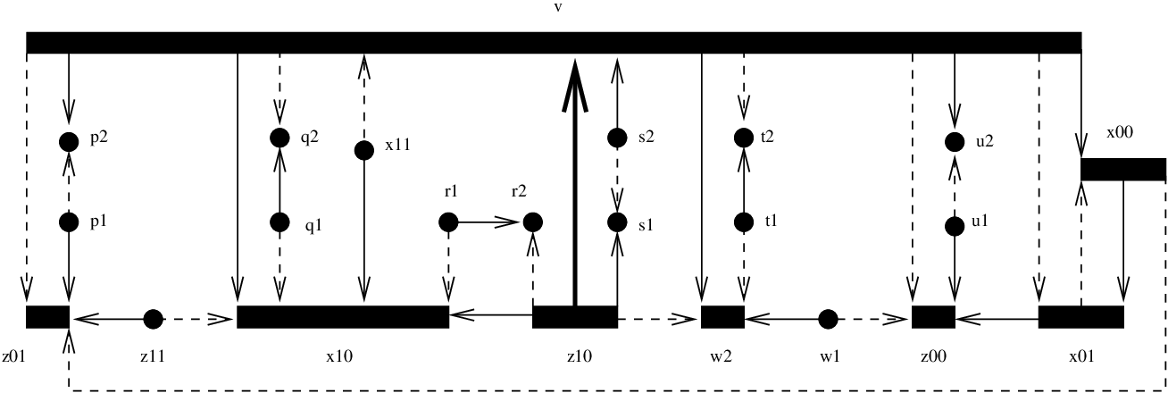
The arcs have disappeared because they have now been switched to agree with . They play no further part in the formation of the canonical path.
Next, we must process the normal 2-circuit
which the eccentric switch has produced (see Figure 6). From Lemma 4.2 we know that the shortcut arc is , and again . Now so falls into case (Nc), and we will perform the shortcut switch last. Our next task is to process the 1-circuit
The set of end-vertices of odd chords which are absent in is . Now is a contiguous substring of , so these vertices are all distinct, and hence has three elements. Thus there will be three phases in the processing of . The first phase is over after just one switch, namely . This produces the next digraph on the canonical path: see Figure 12.

The odd chord has become an interesting arc, so it is included in Figure 12 together with the eccentric arc. Both belong to , and hence they are depicted by a thick unbroken arc. The arcs , , have now been switched to agree with , so they play no further role. Hence we have omitted these arcs from Figure 12.
We now start Phase 2 with the switch , producing the next digraph on the canonical path. See Figure 13. Note that there are four interesting arcs in , namely three odd chords and the eccentric arc. The vertex is omitted from Figure 13 since it has degree zero in the symmetric difference of and . (We will make no further comments on the inclusion of interesting arcs or the omission of isolated vertices for the remaining figures.)

The next step in Phase 2 is the switch , which involves the shortcut arc. This produces the digraph on the canonical path. See Figure 14. Note that has five interesting arcs, namely
This is the maximum possible, by Lemma 5.1. Later we will show that also has the maximum number of bad pairs.

The final step in Phase 2 is the switch , producing the digraph . See Figure 15. Now only one odd chord is interesting, as two have been restored to their original state.

Then we perform Phase 3, which consists of one step: the switch . This produces the digraph which has no interesting odd chords, but still has two interesting arcs, namely the eccentric arc and shortcut arc. See Figure 16.

This completes the processing of the 1-circuit . To complete the processing of the normal 2-circuit we must perform the shortcut switch . This produces the digraph as in Figure 17, with no interesting arcs.

This completes the processing of the normal 2-circuit , and hence it also completes the processing of the eccentric 2-circuit .
It remains to process the remaining circuits in the given order. Each remaining circuit is an alternating 4-cycle, which is processed by a single switch, removing it from the symmetric difference. This gives 6 more switches, specifically
The switches are performed in this order, producing digraphs where . This completes the construction of the canonical path from to corresponding to .
Now let us return to the digraph . We now show that there are 16 bad pairs in with respect to . We redraw in Figure 18, where now solid lines show arcs in and dashed lines show arcs in . Hence solid and dashed arcs play the role of green and yellow arcs, in the terminology of Lemma 5.7. Interesting arcs are still shown with thicker lines.

By tracing around this figure using the circuits given in (18) determined by the pairing , we find that there are 16 bad pairs in with respect to . This is the maximum possible number of bad pairs, as proved in Lemma 5.7. Table 1 shows the bad vertices and the bad pairs of arcs incident with each one.
| bad vertex | bad green pairs | bad yellow pairs |
|---|---|---|
We now make two final comments.
- (i)
In this relatively small example, not many coincidences between the bad vertices are possible. For instance, we know that since is a contiguous substring of , while since is a blue arc in and is a red arc in . In our example, the only coincidences that may occur are that may equal or it may equal . If either holds then the vertex is incident with four bad pairs in , one of each colour and orientation.
- (ii)
This example was constructed to produce a digraph with the maximum number of bad pairs (namely , with 16 bad pairs). This was achieved by letting the interesting arcs all belong to , so that they did not become bad arcs when they became interesting, but instead they created extra bad pairs with respect to . If instead just consisted of the arcs of the eccentric 2-circuit , then any interesting arc would also be a bad arc. (For example, if the eccentric arc had not been an arc of but was absent in both and then in it would become a bad arc with label .) Then the analogue of would be an example of a digraph with the maximum number of bad arcs.
References
- [1] J. Bang-Jensen and G. Gutin, Digraphs: Theory, Algorithms and Applications, 2nd edn., Springer, New York, 2008.
- [2] A. Berger and M. Müller-Hannemann, Uniform sampling of digraphs with a fixed degree sequence, in Graph Theoretic Concepts in Computer Science, Lecture Notes in Computer Science vol. 6410, Springer, Berlin, 2010, pp. 220–231.
- [3] J. Besag and P. Clifford, Generalized Monte Carlo significance tests, Biometrika 76 (1989), 633–642.
- [4] B. Bollobás, A probabilistic proof of an asymptotic formula for the number of labelled regular graphs, European Journal of Combinatorics 1 (1980), 311–316.
- [5] T. Chiang, D. Scholtens, D. Sarkar, R. Gentleman and W. Huber, Coverage and error models of protein-protein interaction data by directed graph analysis, Genome Biology 8 (2007), R186.
- [6] C. Cooper, M.E. Dyer and C. Greenhill, Sampling regular graphs and a peer-to-peer network, Combinatorics, Probability and Computing 16 (2007), 557–593.
- [7] C. Cooper, M. Dyer and A. Handley, The flip Markov chain and a randomising P2P protocol, in Proceedings of the 28th ACM Symposium on Principles of Distributed Computing, ACM Press, New York, 2009.
- [8] P. Diaconis, R. Graham and S.P. Holmes, Statistical problems involving permutations with restricted positions, in State of the Art in Probability and Statistics, Lecture Notes-Monograph Series vol. 36, Institute of Mathematical Statistics, Beachwood, OH, 2001, pp. 195–222.
- [9] P. Diaconis and D. Stroock, Geometric bounds for eigenvalues of Markov chains, Annals of Applied Probability 1 (1991), 36–61.
- [10] P. Diaconis and B. Sturmfels, Algebraic algorithms for sampling from conditional distributions, Annals of Statistics 26 (1998), 363–397.
- [11] P.L. Erdős, I. Miklós and Z. Toroczkai, A simple Havel-Hakimi type algorithm to realize graphical degree sequences of directed graphs, Electronic Journal of Combinatorics 17 (2010), #R66.
- [12] T. Feder, A. Guetz, M. Mihail and A. Saberi, A local switch Markov chain on given degree graphs with application in connectivity of peer-to-peer networks, in Proceedings of the 47th Annual IEEE Symposium on Foundations of Computer Science, IEEE Press, New York, 2006, pp. 69–76.
- [13] C. Hall and A. Carzaniga, Uniform sampling for directed P2P networks, in Proceedings of EURO-PAR 2009 Parallel Processing, Lecture Notes in Computer Science Vol. 5705, Springer, Berlin, 2009, pp. 511–522.
- [14] R. Kannan, P. Tetali and S. Vempala, Simple Markov-chain algorithms for generating bipartite graphs and tournaments, Random Structures and Algorithms 14 (1999), 293–308.
- [15] H. Kim, C.I. Del Genio, K.E. Bassler and Z. Toroczkai, Constructing and sampling directed graphs with given degree sequences, Preprint, 2011. arXiv:1109.4590v1 [physics.soc-ph]
- [16] M.D. LaMar, On uniform sampling simple directed graph realizations of degree sequences (preprint, 2009). arXiv:0912.3834v1 [cs.DM]
- [17] T. Łuczak and J.E. Cohen, Stratigraphy of a random acyclic directed graph: the size of trophic levels in the cascade model, Annals of Applied Probability 3 (1993), 403–420.
- [18] P. Mahlmann and C. Schindelhauer, Peer-to-peer networks based on random transformations of connected regular undirected graphs, in Proceedings of the 17th Annual ACM Symposium on Parallelism for Algorithms and Architectures, ACM Press, New York, 2005, pp. 155–164.
- [19] P. Mahlmann and C. Schindelhauer, Distributed random digraph transformations for peer-to-peer networks, in Proceedings of the 18th annual ACM Symposium on Parallel Algorithms and Architectures, ACM Press, New York, 2006, pp. 308–317.
- [20] C. Martínez, A. Panholzer and H. Prodinger, Generating random derangements, in Proceedings of the Fifth Workshop on Analytic Algorithmics and Combinatorics (ANALCO), SIAM, Philadelphia, PA, 2008, pp. 234–240.
- [21] B.D. McKay, Asymptotics for 0-1 matrices with prescribed line sums, in Enumeration and Design, Academic Press, Toronto, 1984, pp. 225–238.
- [22] B.D. McKay and N.C. Wormald, Uniform generation of random regular graphs of moderate degree, Journal of Algorithms 11 (1990), 52–67.
- [23]
R. Milo, N. Kashtan, S. Itzkovitz, M.E.J. Newman and U. Alon,
On the uniform generation of random graphs with prescribed
degree sequences, Preprint, 2004.
arXiv:cond-mat/0312028v2 [cond-mat.stat-mech] - [24] O. Häggström, Finite Markov chains and algorithmic applications, London Mathematical Society Student Texts vol. 52, Cambridge University Press, Cambridge, 2003.
- [25] A.R. Rao, R. Jana and S. Bandyopadhyay, A Markov chain Monte Carlo method for generating random (0,1)-matrices with given marginals, Sankhy: The Indian Journal of Statistics 58 (1996), 225–242.
- [26] G. Robbins, P. Pattison and P. Wang, Closure, connectivity, degree distributions: Exponential random graph () models for directed social networks, Social Networks 31 (2009), 105–117.
- [27] J. Roberts, Simple methods for simulating sociomatrices with given marginal totals, Social Networks 22 (2000), 273–283.
- [28] H.J. Ryser, Combinatorial Mathematics, Carus Mathematical Monographs, The Mathematical Association of America, 1963.
- [29] A. Sinclair, Improved bounds for mixing rates of Markov chains and multicommodity flow, Combinatorics, Probability and Computing 1 (1992), 351–370.