LTH–896
BU-HEPP 11-01
CASPER 11-01
hep-ph/
Investigation of Quasi–Realistic Heterotic
String Models with Reduced Higgs Spectrum
G. Cleaver** * GeraldCleaver@baylor.edu1, A. Faraggi†† † Faraggi@amtp.liv.ac.uk2, J. Greenwald‡‡ ‡ JaredGreenwald@baylor.edu, D. Moore§§ § DouglasMoore1@baylor.edu, K. Pechan ¶¶ ¶ Kristen.Pechan@physics.tamu.edu, E. Remkus∥∥ ∥ ErikRemkus@baylor.edu and T. Renner **** ** TimothyRenner@baylor.edu
1 CASPER, Department of Physics, Baylor University,
Waco, TX, 76798-7316
2 Department of Mathematical Sciences, University of Liverpool,
Liverpool L69 7ZL
3 Mitchell Institute, Dept. of Physics, Texas A&M,
College Station, TX, 77843-4242
Quasi–realistic heterotic–string models in the free fermionic formulation typically contain an anomalous , which gives rise to a Fayet–Iliopolous term that breaks supersymmetry at the one–loop level in string perturbation theory. Supersymmetry is restored by imposing F– and D–flatness on the vacuum. In [14] we presented a three generation free fermionic standard–like model which did not admit stringent F– and D–flat directions, and argued that the all the moduli in the model are fixed. The particular property of the model was the reduction of the untwisted Higgs spectrum by a combination of symmetric and asymmetric boundary conditions with respect to the internal fermions associated with the compactified dimensions. In this paper we extend the analysis of free fermionic models with reduced Higgs spectrum to the cases in which the symmetry is left unbroken, or is reduced to the flipped subgroup. We show that all the models that we study in this paper do admit stringent flat directions. The only examples of models that do not admit stringent flat directions remain the strandard–like models of ref. [14].
1 Introduction
String theory provides a viable framework to probe the unification of gravity and the gauge interactions. Progress in this endeavor mandates the development of detailed phenomenological models as well as improved understanding of the mathematical structures that underly the theory. On the other hand the Standard Particle Model is compatible with all contemporary terrestrial and extra–terrestrial experimental data. Furthermore, the particle physics data is compatible with the hypothesis that the perturbative Standard Model remains unaltered up to the Planck scale, and that the particle spectrum is embedded in representations of a Grand Unified Theory (GUT). Most appealing in this context is unification in which each Standard Model (SM) generation is embedded in a single spinorial 16 representation.
Heterotic string theory naturally produces models that preserve the grand unified embedding of the Standard Model states [1]. Among the most realistic string models [2, 3, 4, 5, 6, 7, 8, 9] constructed to date are the heterotic–string models in the free fermionic formulation, which are related to toroidal orbifold compactifications [10]. In these models the GUT symmetry is broken directly at the string level, and include: the flipped string models [2]; the SM-like string models [3, 5, 7]; the Pati–Salam string models [4, 9]; and the Left–Right symmetric string models [8] (LRS). Generically, string vacua contain numerous fields beyond the SM states and these must be given sufficiently heavy mass. Heterotic string models necessarily also contain exotic fractionally charged states that are severely constrained by observations. These can be given mass on the order of the Planck scale by Standard Model singlet VEVs [7], or may be entirely absent from the massless spectrum [9]. The free fermionic heterotic string models produced the first known string models in which the matter content of the effective low energy observable sector consists solely of the Minimal Supersymmetric Standard Model (MSSM) [7]. The issue of the supersymmetric moduli space and supersymmetry breaking remains one of the important open issues in string phenomenology.
The relation of free fermion models to orbifolds mandates the production of three untwisted pairs of vectorial representations, which decompose as under and as under the Standard Model gauge group. This presents an excess beyond the two electroweak Higgs doublets that are required in the MSSM. In the Pati–Salam and Standard–like string models either the color triplets or electroweak Higgs doublets from each pair may be projected from the massless spectrum by asymmetric/symmetric boundary conditions with respect to a given twisted plane [12]. Assignment of symmetric and asymmetric boundary conditions in two different basis vectors results in the projection of both color triplets and electroweak doublets and therefore reduces the spectrum without the need to give them heavy mass by singlet VEVs [13, 14]. In this manner entire 10 vectorial pairs can be projected. An additional consequence of the symmetric plus asymmetric assignment is that untwisted singlet states are projected as well and the supersymmetric moduli space is constrained [13, 14].
Standard–like string models that employ the symmetric plus asymmetric boundary condition assignment to reduce the light Higgs spectrum were constructed in refs. [13, 14]. The model constructed in ref. [13] did not admit flat directions that preserve the Standard Model (SM) gauge group. This gave rise to the possibility that the model does not admit supersymmetric flat directions at all. This would be a very interesting situation as it would indicate that supersymmetry is broken perturbatively in such models. In ref. [14] this question was examined further by analyzing the so–called stringent flat directions. It was demonstrated that there exists SM–like string models with reduced untwisted Higgs spectrum, which do not admit stringent flat directions to any order of non-renomalizable superpotential term. This outcome is in contrast to the case of all other quasi–realistic free fermionic models, which have been shown to admit such stringent flat directions.
The question therefore arises whether the absence of stringent flat directions (see Figure 1) in free fermion heterotic–string models with reduced Higgs spectrum is particular to the SM–like models, and whether similar results arise in cases in which the subgroup is broken to an alternative subgroup. In this paper we examine this question by analyzing the - and –flat directions in four models. Three in which the symmetry is broken to the the flipped subgroup and one in which the symmetry remains unbroken. We show that all of these cases admit stringent supersymmetric flat directions. Hence, SM–like models with reduced Higgs spectrum remain the only examples in which stringent flat directions have been shown not to exist.
Our paper is organized as follows: Section 2 contains a review of Free Fermionic Models construction using the NAHE set and additional boundary vectors to control gauge and SUSY breaking. In Section 3, we review the process of flat directions used with EFTs as pertaining to Free Fermionic strings. Here there is a further discussion on stringent -flat directions. The string models in question are reviewed in Sections 4 and 5, where we list the boundary vectors pertaining to each model as well as summarize the flat directions. We conclude our discussion in Section 6 and make comment on the impact of our results on future studies of the Free Fermionic Heterotic Landscape.
2 Free Fermionic Models
In this section we briefly review the construction and structure of the free fermionic standard like models. The notation and further details of the construction of these models are given elsewhere [3, 5, 15, 7, 8, 13]. In the free fermionic formulation of the heterotic string in four dimensions [16] all the world–sheet degrees of freedom, required to cancel the conformal anomaly, are represented in terms of free fermions propagating on the string world–sheet. In the light–cone gauge the world–sheet field content consists of two transverse left– and right–moving space–time coordinate bosons, and , and their left–moving fermionic superpartners, , and additional 62 purely internal Majorana–Weyl fermions, of which 18 are left–moving and 44 are right–moving. The models are constructed by specifying the phases produced by the world–sheet fermions when transported along the torus’ non–contractible loops
| (2.1) |
Each model corresponds to a particular choice of fermion phases consistent with modular invariance and is generated by a set of basis vectors describing the transformation properties of the 64 world–sheet fermions. The physical spectrum is obtained by applying the generalized GSO projections. The GSO projection is administered through the following equations:
| (2.2) | |||
| (2.3) | |||
| (2.4) |
where is the boundary vector defined by eq. 2.1 and is expanded in terms of basis vectors, . For all 64 components of , is the smallest positive integer such that . is the fermion number operator and is equal to for non-periodic fermions and for periodic. After construction of the string model, the low energy effective field theory is obtained by S–matrix elements between external states [17].
The boundary condition basis defining a typical realistic free fermionic heterotic string model is constructed in two stages. The first stage consists of the NAHE set, which is a set of five boundary condition basis vectors, [15]. The gauge group, after imposing the GSO projections induced by the NAHE set, is , with supersymmetry. The NAHE set divides the internal world–sheet fermions in the following way: generate the hidden gauge group, generate the gauge group, while , and generate the three horizontal symmetries. The left–moving states are divided into , , , while , , generate the left–moving world–sheet supersymmetry.
The second stage of the basis construction consists of adding to the NAHE set three additional boundary condition basis vectors. These additional basis vectors reduce the number of generations to three chiral generations, one from each of the sectors , and , and simultaneously break the four dimensional gauge group. The assignment of boundary conditions to breaks to one of its subgroups. Similarly, the hidden symmetry is broken to one of its subgroups. The flavor symmetries in the NAHE–based models are always broken to flavor symmetries, as the breaking of these symmetries is correlated with the number of chiral generations. Three such symmetries are always obtained in the NAHE based free fermionic models from the subgroup of the observable , which is orthogonal to . These are produced by the world–sheet currents (), which are part of the Cartan sub–algebra of the observable . Additional unbroken symmetries, denoted typically by (), arise by pairing two real fermions from the sets , and . The final observable gauge group depends on the number of such pairings. Alternatively, a left–moving real fermion from the sets , and may be paired with its respective right–moving real fermion to form an Ising model operator, in which case the rank of the right–moving gauge group is reduced by one. The reduction of untwisted electroweak Higgs doublets crucially depends on the pairings of the left– and right–moving fermions from the set .
Subsequent to constructing the basis vectors and extracting the massless spectrum, the analysis of the free fermionic models proceeds by calculating the superpotential. The cubic and higher-order terms in the superpotential are obtained by evaluating the correlators
| (2.5) |
where are the fermionic (scalar) components of the vertex operators, using the rules given in [17].
3 Flat Directions of Free Fermions
A common feature of many of the quasi–realistic free fermionic heterotic–string models is the existence of “anomalous” ’s generated from compactification or from gauge group breaking [19]. If multiple ’s are anomalous, the anomaly can always be rotation into a single while the remaining orthogonal ’s all become non-anomalous. This anomalous is broken by the Green–Schwarz–Dine–Seiberg–Witten mechanism [20] in which a potentially large Fayet–Iliopoulos –term is generated by the VEV of the dilaton field. (For the class of free fermionic models under investigation .) Such a –term would, in general, break supersymmetry, unless there is a direction in the scalar potential for which is of opposite sign to and that is –flat with respect to all the non–anomalous gauge symmetries, as well as –flat. If such a direction exists, it will acquire a VEV, canceling the Fayet–Iliopoulos –term, restoring supersymmetry and stabilizing the vacuum.
The –term is formally defined as:
| (3.1) |
where is a generator and is a representation of the group, while the –terms contain fields like squarks, sleptons and Higgs bosons whose VEVs should vanish at this scale for good phenomenology. When the are singlets of all the non–Abelian gauge groups in a model, the set of - and -flat constraints are then given by
| (3.2) | |||
| (3.3) | |||
| (3.4) | |||
| (3.5) |
where are the fields which acquire VEVs of order . The is the superfield formed from the spacetime scalar and the chiral spin-1/2 fermion , while and denote the anomalous and non–anomalous charges and GeV denotes the reduced Planck mass. The solution (i.e. the choice of fields with non–vanishing VEVs) to the set of equations (3.2)–(3.4), though nontrivial, is not unique. Therefore in a typical model there exist a moduli space of solutions to the - and -flatness constraints, which are supersymmetric and degenerate in energy [21]. Much of the study of the superstring model phenomenology (as well as non–string supersymmetric models [22]) involves the analysis and classification of these flat directions. The methods for this analysis in string models have been systematized in [23, 24, 7, 25].
In general it is assumed in the literature that in a given string model there should exist a supersymmetric solution to the - and - flatness constraints. The simpler type of solutions utilize only fields that are singlets of all the non–Abelian groups in a given model (type I solutions). More involved solutions (type II) that utilize non–Abelian fields have also been considered [25], as well as inclusion of non–Abelian fields in systematic methods of analysis [25]. The general expectation that a given model admits a supersymmetric solution arises from analysis of supersymmetric point quantum field theories. In these cases it is known that if supersymmetry is preserved at the classical level, i.e. tree–level in perturbation theory, then there exist index theorems that forbid supersymmetry breaking at the perturbative quantum level [26]. Therefore in point quantum field theories supersymmetry breaking may only be induced by non–perturbative effects [27].
The issue of supersymmetry breaking in the string models that were constructed in refs. [13, 14] merits further investigation. The aim of these models was to construct SM–like string models with reduced untwisted Higgs spectrum. This was achieved by utilizing asymmetric boundary conditions in a basis vector that does not break the symmetry [13]. The consequence is that the entire vectorial 10 representation from the corresponding plane is projected out. The alternative is to utilize a combination of symmetric and asymmetric boundary conditions in basis vectors that break the symmetry to the Pati–Salam gauge group [14]. An unforeseen consequence of the Higgs reduction mechanism of refs. [13, 14] was the simultaneous projection of untwisted singlet fields. Consequently, the moduli space of supersymmetric flat solutions is vastly reduced. In ref. [13] it was concluded that the model under investigation there does not contain supersymmetric flat directions that do not break some of the SM symmetries.
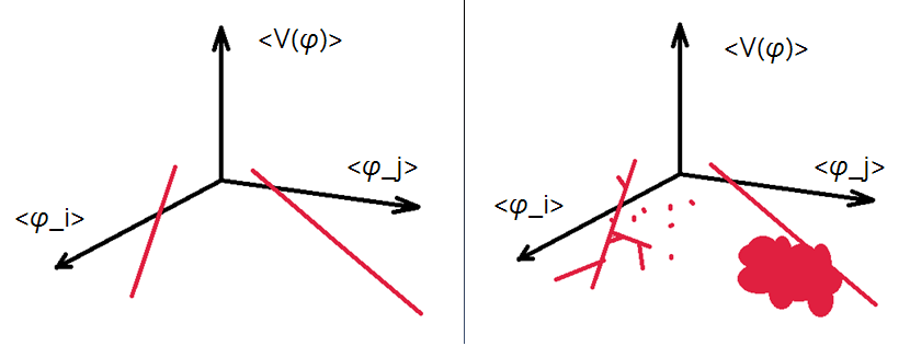
For a given set of flat -term VEVs, an -term will break supersymmetry if its expectation value is non-zero. The scale of supersymmetry breaking is a function of the number of fields in the lowest-order, non-zero component of an -term. Specifically, the lower the number of fields, the higher the energy scale of SUSY breaking. For example, a surviving second order component of an -term breaks SUSY at the string/Planck scale, whereas a order component breaks as needed around the 100 GeV to 1 TeV scale. This SUSY-breaking energy scale is decreased approximately 10 GeV per order increase of the non-zero -term components.
In ref. [14] the issue of superymmetry breaking was investigated further. It was shown that the model studied in [14] does not have -flat directions that can be proven to be -flat to all order, other than through order-by-order analysis. That is, there do not appear to be any -flat directions with stringent -flatness (as defined in [7, 11, 28]). The analysis of the flat directions included all the fields in the string model, i.e. SM singlet states as well as SM charged states. The model of ref. [14] therefore does not contain a –flat direction that is also stringently –flat to all order of non–renormalizable terms. The model may of course still admit non-stringent flat directions that rely on cancellations between superpotential terms. However, past experience suggests that non–stringent flat directions can only hold order by order, and are not maintained to all orders [29, 8]. This is a key difference between the string theory case, in which heavy string modes generate an infinite tower of terms, versus the field theory case in which heavy modes are not integrated out. It was therefore speculated that in this case supersymmetry is not exact, but is in general broken at some order.
The SM–like string models presented in refs [13, 14] contain three chiral generations, charged under the SM gauge group and with the canonical embedding of the weak–hypercharge, one pair of untwisted electroweak Higgs doublets and a cubic level top–quark Yukawa coupling. These string models therefore share some of the phenomenological characteristics of the quasi–realistic free fermionic string models. It may therefore represent an example of a quasi–realistic string model, in which supersymmetry is broken due to the existence of the heavy string modes. The utilization of asymmetric boundary conditions in these models entails that the geometrical moduli in these models are projected out [30]. The Higgs reduction mechanism of refs. [13, 14] further reduces the supersymmetric moduli space, and possibly fixes it completely, while the hidden sector satifies the conditions for the dilaton race–track stabilization mechanism [37, 14]. It is noted that imposing more restrictive phenomenological constraints is correlated with further reduction of the moduli space. The question of interest is therefore whether the restriction of the supersymmetric moduli space is specific to the case of standard–like models. In the next section we investigate the Higgs reduction mechanism in a model with an unbroken symmetry and in three flipped models.
4 The String Models
In this section we present the and flipped string models that utilize the Higgs reduction mechanism of [13, 14]. We first review how the Higgs doublet–triplet splitting mechanism operates in the free fermionic models. For concreteness we illustrate how the mechanism operates in the model of ref. [3].
4.1 Higgs Doublet–Triplet Splitting
An example of a free fermionic SM–like model is given in Table 4.111 1 Only the boundary condition basis vectors beyond the NAHE–set are displayed. .
|
||||||||||||||||||||||||||||||||||||||||||
|
The Higgs doublet–triplet splitting operates as follows [12]. The Neveu–Schwarz sector gives rise to three fields in the 10 representation of . These contain the Higgs electroweak doublets and color triplets. Each of those is charged with respect to one of the horizontal symmetries . Each one of these multiplets is associated, by the horizontal symmetries, with one of the twisted sectors, , and . The doublet–triplet splitting results from the boundary condition basis vectors which break the symmetry to . We can define a quantity in these basis vectors which measures the difference between the boundary conditions assigned to the internal fermions from the set and which are periodic in the vector ,
| (4.11) |
If then the Higgs triplets, and , remain in the massless spectrum while the Higgs doublets, and , are projected out and the opposite occurs for .
The rule in Eq. (4.11) is a generic rule that operates in free fermionic models. The model of eq. (4.1) illustrates this rule. In this model the basis vector that breaks symmetry to is and, with respect to , . Therefore, this model produces three pairs of electroweak Higgs doublets from the Neveu–Schwarz sector, , , and , , and all the untwisted color triplets are projected out. Note also that the vector basis is symmetric with respect to the internal fermions that are periodic in the vectors and, therefore, does not project out the fields in the 10 representation of .
Another possibility is to construct models in which both the Higgs color triplets and electroweak doublets from the Neveu–Schwarz sector are projected out by the GSO projections. This is a viable possibility as we can choose for example
where are the projections due to the basis vectors and respectively. This is desirable as the number of Higgs representations, which generically appear in the massless spectrum, is larger than what is allowed by the low energy phenomenology. The model shown in eq. (4.1) illustrates this possibility
|
||||||||||||||||||||||||||||||||||||||||||
|
Both the basis vectors and break the symmetry to and the basis vector breaks it further to . The basis vector is symmetric with respect to the sector and asymmetric with respect to the sectors and , whereas the basis vector is symmetric with respect to and asymmetric with respect to and . As a consequence of these assignments and of the string doublet–triplet splitting mechanism discussed above, both the untwisted Higgs color triplets and electroweak doublets, with leading coupling to the matter states from the sectors and , are projected out by the generalized GSO projections. At the same time the untwisted color Higgs triplets that couple at leading order to the states from the sector are projected out, whereas the untwisted electroweak Higgs doublets remain in the massless spectrum. Due to the asymmetric boundary conditions in the sector with respect to the sector , the leading Yukawa coupling is that of the up–type quark from the sector to the untwisted electroweak Higgs doublet [6]. Hence, the leading Yukawa term is that of the top quark and only its mass is characterized by the electroweak VEV [6]. The lighter quarks and leptons couple to the light Higgs doublet through higher order non-renormalizable operators that become effective renormalizable operators by the VEVs that are used to cancel the anomalous –term equation [6]. The novelty in the construction of (4.1) is that the reduction of the untwisted Higgs spectrum is obtained by the choice of the boundary condition basis vectors in eq. (4.1), without resorting to analysis of supersymmetric flat directions, whereas in other models it is obtained by the choice of flat directions and analysis of the superpotential [18].
However, the surprising result was that the model does not seem to admit a stringent supersymmetric solution [14]. This appeared to be a consequence of the reduction of untwisted singlet states (denoted by and in that model and in all models presented here), simultaneous with the untwisted Higgs reduction, imposed by the asymmetric/symmetric boundary conditions. We next turn to examine this issue in models in which the symmetry remains unbroken, or is broken to the flipped subgroup.
4.2 An Model
In the previous section we discussed the Higgs reduction mechanism of ref. [13, 14]. We noted that the reduction is achieved by utilizing symmetric and asymmetric boundary conditions in two separate basis vectors. However, the reduction can be obtained if we assign asymmetric boundary conditions in a basis vector that does not break the symmetry. The model in Table 1 is an example of such a model.
| 0 | 0 | 0 | 0 | 1 1 1 1 1 | 1 | 0 | 0 | 0 0 0 0 0 0 0 0 | |
|---|---|---|---|---|---|---|---|---|---|
| 0 | 0 | 0 | 0 | 1 1 1 1 1 | 0 | 1 | 0 | 0 0 0 0 0 0 0 0 | |
| 0 | 0 | 0 | 0 | 1 1 1 1 1 | 1 | 1 | 0 | 1 1 0 0 0 0 0 0 | |
| 0 | 0 | 0 | 0 | 1 1 1 1 1 | 1 | 1 | 1 | 1 0 1 1 1 0 0 0 |
| 1 0 0 1 | 1 0 0 1 | 0 0 0 1 | 1 0 1 1 | 0 0 1 0 | 0 1 1 1 | |
| 0 0 1 0 | 1 0 1 1 | 1 0 1 0 | 1 0 1 0 | 1 0 0 0 | 1 1 0 1 | |
| 0 1 0 0 | 0 1 0 0 | 0 1 0 0 | 0 1 0 0 | 0 1 0 1 | 0 0 0 0 | |
| 0 0 0 0 | 0 0 0 0 | 0 0 0 0 | 0 0 0 0 | 0 0 0 0 | 0 0 0 0 |
We note that in tables 1 and 2 vectors that do not break the symmetry are denoted by with . Basis vectors that break the symmetry in the fliipped models below will be denoted by Greek letters. The last vector in tables 1 and 2 is denoted as to adhere with the notation used in the quasi–realistic free fermionic models [10].
The model defined by Tables 1 and 2 contain three spinorial 16 representations of the GUT group. All untwisted vectorial 10 representations are projected out. The asymmetric boundary conditions in with respect to and projects out the corresponding vectorial representations, whereas the asymmetric boundary condition in with respect to project out the remaining untwisted vectorial representations. The twisted sectors and give rise to vectorial representations and these are the sources of the two pairs of SM Higgs: and .
We note that the model in Tables 1 and 2 is not phenomenologically realistic as it does not contain the heavy Higgs representations needed to break the symmetry to the SM gauge group. Our interest in this model here is to study the existence and characteristic of the (all-order) stringent flat directions. Namely, do they exist, and do they preserve the SM (within the ) gauge group? This question will be discussed in section 5. The states and gauge charges for this model can be found in Table 21 located in Appendix A.
4.3 Flipped Models
Some potentially more realistic models are those with flipped observable sectors. This are listed below in sections: 4.3.1, 4.3.2 and 4.3.3.
4.3.1 Flipped Model 1
This flipped model has additional boundary vectors given in Table 3 and a GSO projection matrix shown in Table 4. The states and gauge charges for this model can be found in Table 22 located in Appendix A. This model is completely lacking in both untwisted and twisted Higgs.
| 0 | 0 | 0 | 0 | 1 1 1 1 1 | 1 | 0 | 0 | 0 0 0 0 0 0 0 0 | |
|---|---|---|---|---|---|---|---|---|---|
| 0 | 0 | 0 | 0 | 1 1 1 1 1 | 1 | 0 | 0 | 0 0 0 0 0 0 0 0 | |
| 0 | 0 | 0 | 0 | 0 0 0 0 |
| 1 0 0 1 | 1 0 0 1 | 0 0 0 1 | 1 0 1 1 | 0 0 1 0 | 0 1 1 1 | |
| 0 0 1 0 | 1 0 1 1 | 1 0 1 0 | 1 0 1 0 | 1 0 0 0 | 1 1 0 1 | |
| 0 1 0 0 | 0 1 0 0 | 0 1 0 0 | 0 1 0 0 | 0 1 0 1 | 0 0 0 0 |
4.3.2 Flipped model 2
This flipped model has additional boundary vectors given in Table 5 and a GSO projection matrix shown in Table 6. The states and gauge charges for this model can be found in Table 23 located in Appendix A. This model has two untwisted Higgs pairs and three more pairs of twisted Higgs.
| 1 | 0 | 0 | 0 | 1 1 1 1 1 | 0 | 1 | 0 | 0 0 0 0 0 0 0 0 | |
|---|---|---|---|---|---|---|---|---|---|
| 1 | 0 | 1 | 0 | 1 1 1 1 1 | 1 | 0 | 0 | 0 0 0 0 0 0 0 0 | |
| 1 | 0 | 0 | 1 |
| 1 0 0 1 | 0 0 0 0 | 0 0 1 0 | 1 0 1 1 | 0 0 0 1 | 0 0 0 1 | |
| 0 0 0 0 | 1 0 0 1 | 1 0 1 1 | 0 0 1 0 | 0 1 0 0 | 0 1 0 0 | |
| 0 1 0 0 | 1 1 0 1 | 0 1 0 0 | 0 1 0 0 | 1 0 1 0 | 0 0 0 0 |
4.3.3 Flipped Model 3
This flipped model has additional boundary vectors given in Table 7 and a GSO projection matrix shown in Table 8. The states and gauge charges for this model can be found in Table 24 located in Appendix A.
| 1 | 1 | 0 | 0 | 1 1 1 1 1 | 0 | 1 | 0 | 0 0 0 0 0 0 0 0 | |
|---|---|---|---|---|---|---|---|---|---|
| 1 | 0 | 1 | 0 | 1 1 1 1 1 | 1 | 0 | 0 | 0 0 0 0 0 0 0 0 | |
| 1 | 0 | 0 | 1 | 1 1 0 0 |
| 1 0 0 1 | 0 0 0 0 | 0 0 1 0 | 1 0 1 1 | 0 0 0 1 | 0 0 0 1 | |
| 0 0 0 0 | 1 0 0 1 | 1 0 1 1 | 0 0 1 0 | 0 1 0 0 | 0 1 0 0 | |
| 0 1 0 0 | 1 1 0 1 | 0 0 0 0 | 1 0 0 1 | 1 1 1 0 | 0 1 0 0 |
This last model produces three generations from the sectors , and and one light Higgs pair from the untwisted sector. The sectors and give rise to heavy Higgs states that are needed to break the gauge symmetry to the Standard Model gauge group. The model admits a cubic level top quark Yukawa coupling of order one. In this respect the model reproduces many of the features of other quasi–realistic flipped string models. Its distinctive characteristic is that two of the untwisted Higgs pairs are projected out due to the asymmetric boundary conditions in and with respect to and .
5 Flat directions
Here we list the results of the flat direction analysis. These lists are by no means exhaustive but are presented just as a “proof of concept”. The model has –flat directions found in Table 9 and all-order stringent –flat directions in Table 10. For this model it was necessary only to investigate type I flat directions (those formed with fields that are singlets under both the observable and hidden sector gauge groups). This is, of course, the preferred option as it is both simpler and computationally less-expensive. The all-order stringent flat directions we found possessed only VEVs of singlets fields and since the SM model is completely contained within that means that the SM remains unbroken here.
Similarly, those flat directions investigated in flipped model #2, were also of type I. The -flat directions for this model can be found in Table 15 and the -flat table can be found in Table 16. We note that the all-order stringent flat directions in Table 16 contain VEVs for one or more generations of anti-electrons. Thus the SM hypercharge is broken in this model. Interestingly, this model contains an exotic negatively-charged electron singlet forming a vector-pair with the corresponding anti-electron (see Table 23).
Both flipped models #1 and #3, however, lacked type I stringent flat directions and required an investigation of those fields which are charged under some non-Abelian gauge representation. For model #1, the failure to produce singlet -flat directions that can solely cancel the Fayet-Iliopoulos term came as a result of all possible directions having an anomalous charge of zero (see Table 11). This condition requires the search for type II directions with negative anomalous charge. This search is a nonlinear process ([14],[31]) and, for the purposes of our investigation, the use of stringency requirements offered a much quicker, and still fruitful, search. The net effect of stringent flatness is that: (1.) at least two fields (including a given field appearing twice) must not take on a VEV or (2.) self-cancellation between components of a non-abelian field must occur. Additionally for model #1, we found (as can be seen in Table 12) non-Abelian -flat directions that were negative. However, these directions failed to yield -flat directions by themselves; this necessitated the mixing of both singlet and non-Abelian -flat directions in order to find all-order stringent -flatness. These mixed -flat directions can be seen in Table 13.
The speed increase from stringent -flat direction searches results from only needing to investigate a finite set of potentially dangerous superpotential terms which determine all-order flatness. The answer to whether or not these terms are dangerous (i.e. they actually exist) comes from the fact that these models are derived from string theory and, therefore, the gauge invariant terms need to also obey Ramon/Neveu-Schwarz (RNS) worldsheet charge conservation. This then makes string-derived models more constrained than the usual QFT-derived ones. These all-order RNS rules can be found in [25].
The - and -flat tables for flipped model #1 can be found in Tables 11–14. Here the gauge group remains unbroken. However, hypercharge is most likely broken in this model since in flipped there is a contribution to hypercharge from an external and all extra appear to be carried by the singlet and/or non-Abelian states acquiring VEVs in the all-order stringent F-flat directions (see Tables 14 and 22). Additionally the hidden sector is broken by the while the remains unbroken.
For flipped model #3, the - and -flat tables can be found in Tables 17–19. We find here that remains unbroken and it is unclear whether hypercharge is broken in the few all-order stringent flat directions calculated. As for the hidden sector, we see from Table 24 that the first and third ’s are broken while the remaining is left unbroken.
| -1 | 0 | 0 | 0 | 0 | 0 | 0 | 0 | 0 | -3 | 0 | 0 | 0 | 1 | 2 | 2 | -2 | 1 | |
| -1 | 0 | -3 | 0 | 0 | 0 | 0 | 0 | 0 | 0 | 0 | 0 | 0 | -2 | 2 | 2 | -2 | 4 | |
| -1 | 0 | 0 | -3 | 0 | 0 | 0 | 0 | 0 | 0 | 0 | 0 | 0 | 4 | 2 | 2 | -2 | -2 | |
| 0 | 1 | 0 | 0 | 0 | 0 | 0 | 0 | 0 | 0 | 0 | 0 | 0 | -2 | 0 | 0 | 0 | 2 | |
| 0 | 0 | 0 | 0 | 0 | 0 | 0 | 0 | 0 | 0 | 1 | 0 | 0 | 0 | 0 | 0 | -1 | 1 | |
| 0 | 0 | 0 | 0 | 0 | 0 | 0 | 0 | 0 | 0 | 0 | 1 | 0 | 0 | 1 | 0 | 0 | -1 | |
| 0 | 0 | 0 | 0 | 1 | 0 | 0 | 0 | 0 | 0 | 0 | 0 | 0 | 1 | 0 | 0 | -1 | 0 | |
| 0 | 0 | 0 | 0 | 0 | 0 | 0 | 0 | 0 | 0 | 0 | 0 | 1 | 0 | 0 | 1 | 0 | 1 | |
| 0 | 0 | 0 | 0 | 0 | 0 | 0 | 1 | 0 | 0 | 0 | 0 | 0 | 1 | 0 | 0 | 0 | -1 | |
| 0 | 0 | 0 | 0 | 0 | 0 | 0 | 0 | 1 | 0 | 0 | 0 | 0 | 1 | 0 | 0 | 0 | -1 | |
| 0 | 0 | 0 | 0 | 0 | 1 | 0 | 0 | 0 | 0 | 0 | 0 | 0 | -1 | 1 | 0 | 0 | 0 | |
| 0 | 0 | 0 | 0 | 0 | 0 | 1 | 0 | 0 | 0 | 0 | 0 | 0 | 1 | 0 | 1 | 0 | 0 |
| FD | |||||||||||||
|---|---|---|---|---|---|---|---|---|---|---|---|---|---|
| 1 | -49 | 0 | -3 | -144 | -98 | 0 | 0 | 0 | 92 | 98 | 0 | -98 | -92 |
| 2 | -1 | 0 | -1 | -2 | -2 | 0 | 0 | 0 | 0 | 2 | 0 | -2 | 0 |
| 3 | -1 | 0 | 0 | -3 | -4 | 0 | 0 | 0 | 0 | 2 | -2 | -2 | -2 |
| 4 | -1 | 0 | -1 | 0 | 0 | -2 | 0 | -2 | 0 | 2 | 0 | -2 | 0 |
| 5 | -2 | 0 | -3 | -1 | 0 | -2 | 0 | -4 | 0 | 4 | 0 | -4 | 0 |
| 6 | -1 | 0 | 0 | 1 | 0 | -4 | 0 | -2 | 0 | 2 | 0 | -2 | 0 |
| 7 | -1 | 0 | 0 | -1 | -2 | -2 | 0 | 0 | 0 | 2 | 0 | -2 | 0 |
| 8 | -2 | 0 | -1 | -3 | -4 | -2 | 0 | 0 | 0 | 4 | 0 | -4 | 0 |
| 9 | -1 | 0 | 1 | 0 | -2 | -4 | 0 | 0 | 0 | 2 | 0 | -2 | 0 |
| 10 | -2 | 1 | 0 | 0 | 0 | -6 | 0 | -4 | 0 | 4 | 0 | -4 | 0 |
| 11 | -5 | 1 | 0 | 3 | 0 | -18 | 0 | -10 | 0 | 10 | 0 | -10 | 0 |
| 12 | -2 | -1 | 0 | 0 | -4 | -6 | 0 | 0 | 0 | 4 | 0 | -4 | 0 |
| 13 | -5 | -1 | 0 | -3 | -10 | -12 | 0 | 0 | 0 | 10 | 0 | -10 | 0 |
| 14 | -1 | 0 | 0 | 0 | 0 | -3 | -2 | -3 | 1 | 0 | -1 | -2 | 0 |
| 15 | -1 | 0 | 0 | 1 | 0 | -4 | -2 | -4 | 0 | 0 | -2 | -2 | 0 |
| 0 | 1 | 0 | 0 | 0 | 0 | 0 | 0 | 0 | 0 | 0 | 0 | -2 | 0 | 0 | 0 | 2 | -2 | 0 | 0 | 0 | 0 | 0 | |
| 0 | 0 | 0 | 0 | 0 | 0 | 0 | 0 | 1 | 0 | 0 | 0 | -1 | 0 | 0 | 0 | 1 | 0 | 0 | 0 | 0 | 0 | 0 | |
| 0 | 0 | 0 | 0 | 0 | 0 | 0 | 0 | 0 | 0 | 0 | 0 | 0 | 1 | 0 | 0 | -1 | -1 | 0 | 0 | 0 | 0 | 0 | |
| 0 | 0 | 0 | 0 | 0 | 0 | 0 | 0 | 0 | 0 | 0 | 1 | -1 | 0 | 0 | 0 | -1 | -1 | 0 | 0 | 0 | 0 | 0 | |
| 0 | 0 | 0 | 0 | 0 | 0 | 0 | 0 | 0 | 0 | 0 | 0 | 0 | 0 | 0 | 1 | -1 | 0 | 0 | 0 | 0 | 0 | 0 | |
| 0 | 0 | 0 | 0 | 0 | 0 | 0 | 0 | 0 | 0 | 0 | 0 | 0 | 0 | 1 | 0 | 2 | 0 | 0 | 0 | 0 | 0 | 0 | |
| 0 | 0 | 0 | 0 | 0 | 0 | 0 | 0 | 0 | 0 | 1 | 0 | -1 | 0 | 0 | 0 | 1 | -1 | 0 | 0 | 0 | 0 | 0 | |
| 0 | 0 | 0 | 0 | 0 | 0 | 0 | 0 | 0 | 0 | 0 | 0 | 0 | 0 | 0 | 0 | 1 | -1 | 0 | 1 | 0 | 0 | 0 | |
| 0 | 0 | 0 | 0 | 0 | 1 | 0 | 0 | 0 | 0 | 0 | 0 | -1 | 0 | 0 | 0 | 0 | -1 | 0 | 0 | 0 | 0 | 0 | |
| 0 | 0 | 0 | 0 | 0 | 0 | 0 | 0 | 0 | 1 | 0 | 0 | -1 | 0 | 0 | 0 | 1 | -1 | 0 | 0 | 0 | 0 | 0 | |
| 0 | 0 | 0 | 0 | 0 | 0 | 0 | 1 | 0 | 0 | 0 | 0 | -1 | 0 | 0 | 0 | 2 | -1 | 0 | 0 | 0 | 0 | 0 | |
| 0 | 0 | 0 | 0 | 1 | 0 | 0 | 0 | 0 | 0 | 0 | 0 | -2 | 0 | 0 | 0 | 1 | -1 | 0 | 0 | 0 | 0 | 0 | |
| 0 | 0 | 0 | 0 | 0 | 0 | 1 | 0 | 0 | 0 | 0 | 0 | -1 | 0 | 0 | 0 | 0 | -1 | 0 | 0 | 0 | 0 | 0 | |
| 0 | 0 | 0 | 0 | 0 | 0 | 0 | 0 | 0 | 0 | 0 | 0 | 0 | 0 | 0 | 0 | -2 | 0 | 1 | 0 | 0 | 0 | 0 | |
| 0 | 0 | 0 | 1 | 0 | 0 | 0 | 0 | 0 | 0 | 0 | 0 | -2 | 0 | 0 | 0 | 0 | -2 | 0 | 0 | 0 | 0 | 0 | |
| 0 | 0 | 1 | 0 | 0 | 0 | 0 | 0 | 0 | 0 | 0 | 0 | -2 | 0 | 0 | 0 | 1 | -2 | 0 | 0 | 0 | 0 | 0 |
| 2 | 3 | -3 | -3 | 0 | 0 | 0 | 0 | 5 | 0 | 0 | 0 | 0 | 0 | 5 | 0 | 0 | |
| 2 | 3 | -3 | -3 | 5 | 0 | 0 | 0 | 0 | 0 | 0 | 0 | 0 | 0 | 0 | 0 | 0 | |
| 2 | 3 | -3 | -3 | 0 | 0 | 5 | 0 | 0 | 0 | 0 | 0 | 0 | 0 | 0 | 5 | 0 | |
| 1 | 0 | 0 | -2 | 0 | 0 | 0 | 0 | 0 | 0 | 0 | 0 | 0 | 1 | 1 | 1 | 0 | |
| 1 | 0 | -2 | 0 | 0 | 0 | 0 | 0 | 0 | 0 | 0 | 0 | 1 | 0 | 1 | 0 | 1 | |
| 2 | 2 | -4 | -4 | 0 | 0 | 0 | 0 | 0 | 0 | 1 | 0 | 0 | 0 | 3 | 2 | 2 | |
| 4 | -9 | -1 | -1 | 0 | 0 | 0 | 0 | 0 | 5 | 0 | 0 | 0 | 0 | 5 | 0 | 0 | |
| -6 | -9 | 19 | 9 | 0 | 0 | 0 | 5 | 0 | 0 | 0 | 0 | 0 | 0 | -10 | -5 | -10 | |
| -1 | 0 | 2 | 2 | 0 | 0 | 0 | 0 | 0 | 0 | 0 | 1 | 0 | 0 | -2 | -1 | -1 | |
| -6 | -9 | 9 | 19 | 0 | 5 | 0 | 0 | 0 | 0 | 0 | 0 | 0 | 0 | -10 | -10 | -5 |
| 0 | 0 | 0 | 0 | 0 | 0 | 0 | -1 | 1 | 1 | 0 | 0 | 0 | 0 | 0 | 1 | 0 | 0 | -1 | 0 | 0 | |
|---|---|---|---|---|---|---|---|---|---|---|---|---|---|---|---|---|---|---|---|---|---|
| 0 | 0 | 0 | 0 | 0 | 0 | 0 | -1 | 1 | 1 | 0 | 0 | 0 | 1 | 0 | 0 | 0 | 0 | 0 | -1 | 0 | |
| 0 | 0 | 0 | 0 | 0 | 0 | 0 | -1 | 1 | 1 | 0 | 0 | 1 | 0 | 0 | 0 | 0 | 0 | 0 | 0 | -1 | |
| 0 | 0 | 0 | 0 | 0 | 0 | 0 | 2 | 0 | -2 | 1 | 0 | 0 | 0 | 0 | 0 | 0 | 0 | 0 | 1 | 0 | |
| 0 | 0 | 0 | 0 | 0 | 0 | 0 | 2 | -2 | 0 | 0 | 1 | 0 | 0 | 0 | 0 | 0 | 0 | 0 | 0 | 1 | |
| 0 | 0 | 1 | -1 | 0 | 0 | 0 | 0 | 0 | 0 | 0 | 0 | 0 | 0 | 0 | 0 | 0 | 0 | 0 | 0 | 0 | |
| 0 | -1 | 0 | 1 | 0 | 0 | 0 | 2 | 0 | -2 | 0 | 0 | 0 | 0 | 0 | 0 | 0 | 0 | 0 | 0 | 0 | |
| 0 | 0 | 0 | 1 | 0 | 0 | 0 | 0 | 1 | -1 | 0 | 0 | 0 | 0 | 0 | 0 | 0 | 0 | 0 | 0 | 0 | |
| 1 | 0 | 0 | 0 | 2 | -1 | -1 | 0 | 0 | 0 | 0 | 0 | 0 | 0 | 0 | 0 | 0 | 3 | 0 | 0 | 0 | |
| 1 | 0 | 0 | 0 | -1 | -1 | 2 | 0 | 0 | 0 | 0 | 0 | 0 | 0 | 3 | 0 | 0 | 0 | 0 | 0 | 0 | |
| 1 | 0 | 0 | 0 | -1 | 2 | -1 | 0 | 0 | 0 | 0 | 0 | 0 | 0 | 0 | 0 | 3 | 0 | 0 | 0 | 0 |
| FD | |||||||||||||
|---|---|---|---|---|---|---|---|---|---|---|---|---|---|
| 1 | -14 | -2 | 6 | 0 | -23 | -1 | -1 | 6 | 1 | 22 | 0 | 16 | 15 |
| 2 | -1 | -2 | 6 | 0 | 0 | -42 | -42 | 15 | 0 | 18 | 31 | 34 | 34 |
| 3 | -14 | 0 | -3 | -3 | -1 | -13 | -7 | 7 | 0 | 21 | 0 | 14 | 14 |
| 4 | -15 | 0 | -3 | -3 | -1 | -15 | -9 | 8 | 0 | 23 | 1 | 16 | 16 |
| 5 | -16 | 1 | -3 | 0 | 0 | -12 | -12 | 9 | 0 | 24 | 1 | 16 | 16 |
| 6 | -1 | 0 | 33 | -33 | -44 | -68 | -2 | 23 | 0 | 24 | 45 | 46 | 46 |
| 7 | -1 | 0 | 30 | -30 | -42 | -60 | 0 | 21 | 0 | 24 | 39 | -42 | 42 |
| 8 | -1 | 0 | 9 | -9 | 0 | -56 | -38 | 19 | 0 | 20 | 37 | 38 | 38 |
| 9 | -14 | 0 | 3 | -3 | -13 | -7 | -1 | 7 | 0 | 21 | 0 | 14 | 14 |
| -1 | 0 | -5 | -3 | -3 | -2 | 1 | 7 | -4 | 0 | 3 | 0 | 0 | 0 | 0 | 0 | 0 | 0 | 0 | 0 | 0 | 0 | 0 | 0 | 0 | 0 | 0 | 0 | 0 | |
| -1 | 0 | -2 | -3 | -3 | -2 | -2 | 7 | -4 | 0 | 0 | 0 | 0 | 0 | 3 | 0 | 0 | 0 | 0 | 0 | 0 | 0 | 0 | 0 | 0 | 0 | 0 | 0 | 0 | |
| -1 | 0 | -5 | -3 | -3 | -2 | -2 | 7 | -1 | 0 | 0 | 0 | 0 | 3 | 0 | 0 | 0 | 0 | 0 | 0 | 0 | 0 | 0 | 0 | 0 | 0 | 0 | 0 | 0 | |
| -1 | 0 | 1 | -3 | -3 | 1 | -2 | 4 | -1 | 0 | 0 | 0 | 0 | 0 | 0 | 0 | 0 | 0 | 0 | 0 | 0 | 0 | 3 | 0 | 0 | 0 | 0 | 0 | 0 | |
| -1 | -3 | -2 | 0 | -3 | -2 | 1 | 1 | -1 | 0 | 0 | 0 | 0 | 0 | 0 | 0 | 0 | 0 | 0 | 0 | 0 | 0 | 0 | 0 | 0 | 0 | 0 | 0 | 0 | |
| 1 | 0 | 2 | 0 | 0 | 2 | -1 | -1 | 1 | 0 | 0 | 0 | 0 | 0 | 0 | 0 | 0 | 0 | 0 | 0 | 3 | 0 | 0 | 0 | 0 | 0 | 0 | 0 | 0 | |
| 1 | 0 | 2 | 3 | 3 | -4 | 2 | -1 | -2 | 0 | 0 | 0 | 0 | 0 | 0 | 0 | 0 | 0 | 0 | 0 | 0 | 0 | 0 | 0 | 0 | 0 | 0 | 0 | 3 | |
| 1 | 0 | -1 | 3 | 3 | -4 | 2 | -1 | 1 | 0 | 0 | 0 | 0 | 0 | 0 | 0 | 0 | 0 | 0 | 0 | 0 | 0 | 0 | 0 | 0 | 0 | 0 | 3 | 0 | |
| 1 | 0 | -1 | 3 | 3 | -4 | 5 | -1 | -2 | 0 | 0 | 0 | 0 | 0 | 0 | 0 | 0 | 0 | 0 | 0 | 0 | 0 | 0 | 3 | 0 | 0 | 0 | 0 | 0 | |
| 0 | 0 | 1 | 0 | 0 | 1 | -2 | 0 | 1 | 0 | 0 | 0 | 0 | 0 | 0 | 0 | 0 | 1 | 0 | 0 | 0 | 0 | 0 | 0 | 0 | 0 | 0 | 0 | 0 | |
| 0 | 0 | -1 | -1 | 0 | -1 | 1 | 1 | 0 | 0 | 0 | 0 | 0 | 0 | 0 | 0 | 0 | 0 | 0 | 0 | 0 | 1 | 0 | 0 | 0 | 0 | 0 | 0 | 0 | |
| 0 | 0 | -1 | 0 | 0 | 1 | 0 | 0 | 1 | 0 | 0 | 0 | 0 | 0 | 0 | 0 | 0 | 0 | 0 | 1 | 0 | 0 | 0 | 0 | 0 | 0 | 0 | 0 | 0 | |
| 0 | 0 | 1 | 0 | 0 | 1 | 0 | 0 | -1 | 0 | 0 | 0 | 0 | 0 | 0 | 0 | 0 | 0 | 1 | 0 | 0 | 0 | 0 | 0 | 0 | 0 | 0 | 0 | 0 | |
| 0 | 0 | 1 | 1 | 1 | 1 | 0 | -2 | 1 | 0 | 0 | 0 | 0 | 0 | 0 | 0 | 0 | 0 | 0 | 0 | 0 | 0 | 0 | 0 | 0 | 0 | 1 | 0 | 0 | |
| 0 | 0 | -1 | 1 | 0 | -1 | 1 | -1 | 0 | 1 | 0 | 0 | 0 | 0 | 0 | 0 | 0 | 0 | 0 | 0 | 0 | 0 | 0 | 0 | 0 | 0 | 0 | 0 | 0 | |
| 0 | 0 | 0 | 1 | 0 | 1 | 0 | -2 | 1 | 0 | 0 | 1 | 0 | 0 | 0 | 0 | 0 | 0 | 0 | 0 | 0 | 0 | 0 | 0 | 0 | 0 | 0 | 0 | 0 | |
| 0 | 0 | -1 | 1 | -1 | 0 | 0 | 0 | 0 | 0 | 0 | 0 | 1 | 0 | 0 | 0 | 0 | 0 | 0 | 0 | 0 | 0 | 0 | 0 | 0 | 0 | 0 | 0 | 0 | |
| 0 | 0 | -1 | -1 | -1 | 0 | 0 | 2 | 0 | 0 | 0 | 0 | 0 | 0 | 0 | 0 | 0 | 0 | 0 | 0 | 0 | 0 | 0 | 0 | 0 | 1 | 0 | 0 | 0 | |
| 0 | 0 | -1 | 0 | -2 | -1 | 0 | 2 | -1 | 0 | 0 | 0 | 0 | 0 | 0 | 1 | 0 | 0 | 0 | 0 | 0 | 0 | 0 | 0 | 0 | 0 | 0 | 0 | 0 | |
| 0 | 0 | 0 | -1 | 0 | 1 | 0 | 0 | 1 | 0 | 0 | 0 | 0 | 0 | 0 | 0 | 0 | 0 | 0 | 0 | 0 | 0 | 0 | 0 | 1 | 0 | 0 | 0 | 0 | |
| 0 | 0 | 1 | 0 | 0 | 1 | 0 | -2 | 1 | 0 | 0 | 0 | 0 | 0 | 0 | 0 | 1 | 0 | 0 | 0 | 0 | 0 | 0 | 0 | 0 | 0 | 0 | 0 | 0 |
| FD | |||||||||||||||||
|---|---|---|---|---|---|---|---|---|---|---|---|---|---|---|---|---|---|
| 1 | -3 | 0 | -4 | 1 | 1 | 4 | 0 | 1 | 0 | 6 | 0 | 2 | 1 | 0 | 0 | 0 | 10 |
| 2 | -3 | -6 | -4 | 1 | -5 | -2 | 0 | 1 | 0 | 0 | 0 | 2 | 1 | 0 | 0 | 0 | 4 |
| 3 | -1 | 0 | -8 | 1 | -3 | -2 | 0 | 3 | 0 | 0 | 4 | 4 | 1 | 0 | 2 | 0 | 0 |
| 4 | -2 | 0 | -17 | 5 | -6 | -1 | 0 | 0 | 4 | 0 | 11 | 9 | 1 | 0 | 4 | 0 | 0 |
| 5 | -1 | 0 | -8 | -7 | -3 | -2 | 0 | 11 | 0 | 0 | 0 | 4 | 1 | 0 | 2 | 4 | 0 |
| 6 | -2 | -3 | -10 | -3 | -6 | 0 | 0 | 8 | 0 | 1 | 0 | 1 | 1 | 4 | 0 | 0 | 0 |
| 7 | -4 | -7 | -4 | 2 | -5 | -1 | 0 | 0 | 0 | 1 | 0 | 2 | 2 | 0 | 0 | 0 | 7 |
| 8 | -2 | -2 | -2 | 1 | -1 | 1 | 0 | 0 | 0 | 2 | 0 | 1 | 1 | 0 | 0 | 0 | 5 |
| 9 | -3 | -4 | -4 | 1 | 3 | 0 | 0 | 1 | 0 | 2 | 0 | 2 | 1 | 0 | 0 | 0 | 6 |
| 10 | -4 | -6 | -5 | 1 | -4 | 0 | 0 | 0 | 1 | 2 | 0 | 3 | 1 | 0 | 0 | 0 | 8 |
| 11 | -3 | -1 | -4 | 1 | 0 | 3 | 0 | 1 | 0 | 5 | 0 | 2 | 1 | 0 | 0 | 0 | 9 |
| 12 | -4 | -2 | -5 | 2 | 0 | 4 | 1 | 0 | 0 | 7 | 0 | 2 | 1 | 0 | 0 | 0 | 12 |
| 13 | -4 | -2 | -5 | 2 | 0 | 4 | 1 | 0 | 0 | 7 | 0 | 2 | 1 | 0 | 0 | 0 | 12 |
| 14 | -4 | -7 | -11 | 2 | -12 | -1 | 0 | 0 | 0 | 1 | 7 | 2 | 2 | 0 | 0 | 0 | 0 |
| 1 | 0 | 7 | 0 | -2 | -2 | 1 | 0 | 0 | 0 | 6 | 0 | 0 | 0 | 0 | 6 | |
| 1 | 0 | 4 | -3 | -2 | 1 | -2 | 0 | 0 | 0 | 0 | 0 | 6 | 0 | 0 | 6 | |
| 1 | 0 | 4 | -3 | 1 | -2 | -2 | 0 | 0 | 0 | 0 | 0 | 0 | 0 | 6 | 6 | |
| 0 | 0 | 0 | 0 | -1 | 1 | 0 | 0 | 0 | 0 | 0 | 0 | 0 | 2 | 0 | -2 | |
| 0 | 1 | -1 | -1 | 1 | 0 | 0 | 0 | 0 | 0 | 0 | 0 | 0 | 0 | 0 | 0 | |
| 0 | 0 | -1 | 0 | 0 | 0 | -1 | 2 | 0 | -2 | 0 | 0 | 0 | 0 | 0 | 0 | |
| 0 | 0 | 1 | 1 | -1 | 0 | 1 | 0 | 0 | 0 | 0 | 2 | 0 | 0 | 0 | -2 | |
| 0 | 0 | 0 | 0 | -1 | -1 | 0 | 0 | 2 | -2 | 0 | 0 | 0 | 0 | 0 | 0 |
| F1 | f1b | F2 | f2b | F3 | f3b | h1 | h2 | |||||||||||||||||||
| H1(1b) | H2(3) | H4(5) | H6(7) | H8 | H9 | H10 | H11 | H12 | H13 | H14 | H15 | H16 | H17 | H18 | H19 | H20 | H21 | H22 | H23 | H24 | H25 | H26 | H27 | |||
| H28 | H29 | H30 | H31 | H32 | H33 | H34 | H35 | H36 | H37 | H38 | H39 | H40 | H41 | H42 | H43 | H44 | H45 | H46 | H47 | |||||||
| -1 | 0 | -16 | -15 | 11 | -1 | 8 | 0 | 0 | 0 | 0 | 0 | 0 | 0 | 0 | 0 | 0 | 0 | 0 | 0 | 0 | 0 | 0 | 15 | |||
| 0 | 0 | 0 | 0 | 0 | 0 | 0 | 0 | 0 | 0 | 0 | 0 | 0 | 0 | 0 | 0 | 0 | 0 | 0 | 0 | 0 | 0 | 0 | 0 | |||
| 0 | 12 | 0 | 0 | 0 | 0 | 0 | 0 | 0 | 0 | 0 | 0 | 0 | 0 | 0 | 0 | 0 | 12 | 0 | 0 | |||||||
| -1 | 0 | -16 | -15 | 11 | 14 | -7 | 0 | 0 | 0 | 0 | 0 | 0 | 0 | 0 | 0 | 0 | 0 | 0 | 0 | 0 | 0 | 15 | 0 | |||
| 0 | 0 | 0 | 0 | 0 | 0 | 0 | 0 | 0 | 0 | 0 | 0 | 0 | 0 | 0 | 0 | 0 | 0 | 0 | 0 | 0 | 0 | 0 | 0 | |||
| 0 | 12 | 0 | 0 | 0 | 0 | 0 | 0 | 0 | 0 | 0 | 0 | 0 | 0 | 0 | 0 | 0 | 12 | 0 | 0 | |||||||
| 1 | 0 | 22 | 21 | -11 | -2 | 4 | 0 | 0 | 0 | 12 | 0 | 0 | 0 | 0 | 0 | 0 | 0 | 0 | 0 | 0 | 0 | 0 | 0 | |||
| 0 | 0 | 0 | 0 | 0 | 0 | 0 | 0 | 0 | 0 | 0 | 0 | 0 | 0 | 0 | 0 | 0 | 0 | 0 | 0 | 0 | 0 | 0 | 0 | |||
| 0 | 0 | 0 | 0 | 0 | 0 | 0 | 0 | 0 | 0 | 0 | 0 | 0 | 0 | 0 | 0 | 0 | -24 | 0 | 0 | |||||||
| 1 | 0 | -2 | -15 | 1 | -2 | 4 | 0 | 0 | 0 | 0 | 12 | 0 | 0 | 0 | 0 | 0 | 0 | 0 | 0 | 0 | 0 | 0 | 0 | |||
| 0 | 0 | 0 | 0 | 0 | 0 | 0 | 0 | 0 | 0 | 0 | 0 | 0 | 0 | 0 | 0 | 0 | 0 | 0 | 0 | 0 | 0 | 0 | 0 | |||
| 0 | 0 | 0 | 0 | 0 | 0 | 0 | 0 | 0 | 0 | 0 | 0 | 0 | 0 | 0 | 0 | 0 | 24 | 0 | 0 | |||||||
| 1 | 0 | -8 | -21 | 1 | 4 | -2 | 0 | 0 | 0 | 0 | 0 | 0 | 12 | 0 | 0 | 0 | 0 | 0 | 0 | 0 | 0 | 0 | 0 | |||
| 0 | 0 | 0 | 0 | 0 | 0 | 0 | 0 | 0 | 0 | 0 | 0 | 0 | 0 | 0 | 0 | 0 | 0 | 0 | 0 | 0 | 0 | 0 | 0 | |||
| 0 | 0 | 0 | 0 | 0 | 0 | 0 | 0 | 0 | 0 | 0 | 0 | 0 | 0 | 0 | 0 | 0 | 24 | 0 | 0 | |||||||
| 1 | 0 | -4 | -11 | 7 | -2 | -2 | 0 | 0 | 0 | 0 | 0 | 0 | 0 | 0 | 12 | 0 | 0 | 0 | 0 | 0 | 0 | 0 | 0 | |||
| 0 | 0 | 0 | 0 | 0 | 0 | 0 | 0 | 0 | 0 | 0 | 0 | 0 | 0 | 0 | 0 | 0 | 0 | 0 | 0 | 0 | 0 | 0 | 0 | |||
| 0 | 0 | 0 | 0 | 0 | 0 | 0 | 0 | 0 | 0 | 0 | 0 | 0 | 0 | 0 | 0 | 0 | 24 | 0 | 0 | |||||||
| 1 | 0 | 46 | 75 | -41 | -14 | -8 | 0 | 0 | 0 | 0 | 0 | 0 | 0 | 0 | 0 | 0 | 0 | 0 | 60 | 0 | 0 | 0 | 0 | |||
| 0 | 0 | 0 | 0 | 0 | 0 | 0 | 0 | 0 | 0 | 0 | 0 | 0 | 0 | 0 | 0 | 0 | 0 | 0 | 0 | 0 | 0 | 0 | 0 | |||
| 0 | -36 | 0 | 0 | 0 | 0 | 0 | 0 | 0 | 0 | 0 | 0 | 0 | 0 | 0 | 0 | 0 | -36 | 0 | 0 | |||||||
| 1 | 0 | 10 | 3 | -5 | -2 | 4 | 0 | 0 | 0 | 0 | 0 | 0 | 0 | 0 | 0 | 0 | 0 | 0 | 0 | 0 | 0 | 0 | 0 | |||
| 0 | 0 | 12 | 0 | 0 | 0 | 0 | 0 | 0 | 0 | 0 | 0 | 0 | 0 | 0 | 0 | 0 | 0 | 0 | 0 | 0 | 0 | 0 | 0 | |||
| 0 | 0 | 0 | 0 | 0 | 0 | 0 | 0 | 0 | 0 | 0 | 0 | 0 | 0 | 0 | 0 | 0 | 0 | 0 | 0 | |||||||
| 1 | 0 | 76 | 75 | -71 | -44 | 22 | 0 | 0 | 0 | 0 | 0 | 0 | 0 | 0 | 0 | 0 | 0 | 0 | 0 | 60 | 0 | 0 | 0 | |||
| 0 | 0 | 0 | 0 | 0 | 0 | 0 | 0 | 0 | 0 | 0 | 0 | 0 | 0 | 0 | 0 | 0 | 0 | 0 | 0 | 0 | 0 | 0 | 0 | |||
| 0 | -72 | 0 | 0 | 0 | 0 | 0 | 0 | 0 | 0 | 0 | 0 | 0 | 0 | 0 | 0 | 0 | -72 | 0 | 0 | |||||||
| 1 | 0 | -26 | -33 | 19 | 10 | -8 | 12 | 0 | 0 | 0 | 0 | 0 | 0 | 0 | 0 | 0 | 0 | 0 | 0 | 0 | 0 | 0 | 0 | |||
| 0 | 0 | 0 | 0 | 0 | 0 | 0 | 0 | 0 | 0 | 0 | 0 | 0 | 0 | 0 | 0 | 0 | 0 | 0 | 0 | 0 | 0 | 0 | 0 | |||
| 0 | 24 | 0 | 0 | 0 | 0 | 0 | 0 | 0 | 0 | 0 | 0 | 0 | 0 | 0 | 0 | 0 | 24 | 0 | 0 | |||||||
| 1 | 0 | 4 | -3 | 1 | -2 | -2 | 0 | 0 | 0 | 0 | 0 | 0 | 0 | 0 | 0 | 0 | 0 | 0 | 0 | 0 | 0 | 0 | 0 | |||
| 0 | 0 | 0 | 0 | 0 | 0 | 0 | 0 | 0 | 0 | 0 | 0 | 0 | 0 | 0 | 0 | 0 | 0 | 0 | 0 | 0 | 0 | 0 | 0 | |||
| 0 | 0 | 0 | 12 | 0 | 0 | 0 | 0 | 0 | 0 | 0 | 0 | 0 | 0 | 0 | 0 | 0 | 0 | 0 | 0 | |||||||
| 1 | 0 | 4 | 3 | 1 | 4 | -2 | 0 | 0 | 0 | 0 | 0 | 0 | 0 | 0 | 0 | 0 | 0 | 0 | 0 | 0 | 0 | 0 | 0 | |||
| 0 | 0 | 0 | 0 | 0 | 0 | 0 | 0 | 0 | 0 | 0 | 0 | 0 | 0 | 0 | 0 | 0 | 0 | 0 | 0 | 0 | 0 | 0 | 0 | |||
| 0 | 0 | 0 | 0 | 0 | 0 | 0 | 0 | 0 | 0 | 0 | 12 | 0 | 0 | 0 | 0 | 0 | 0 | 0 | 0 | |||||||
| 1 | 0 | -2 | -3 | 1 | -2 | 4 | 0 | 0 | 0 | 0 | 0 | 0 | 0 | 0 | 0 | 0 | 0 | 0 | 0 | 0 | 0 | 0 | 0 | |||
| 0 | 0 | 0 | 0 | 0 | 0 | 0 | 0 | 0 | 0 | 0 | 0 | 0 | 0 | 0 | 0 | 0 | 0 | 0 | 0 | 0 | 0 | 0 | 0 | |||
| 0 | 0 | 0 | 0 | 0 | 0 | 0 | 12 | 0 | 0 | 0 | 0 | 0 | 0 | 0 | 0 | 0 | 0 | 0 | 0 | |||||||
| 1 | 0 | -2 | -3 | 1 | -2 | 4 | 0 | 0 | 0 | 0 | 0 | 0 | 0 | 0 | 0 | 0 | 0 | 0 | 0 | 0 | 0 | 0 | 0 | |||
| 0 | 0 | 0 | 0 | 0 | 0 | 0 | 0 | 0 | 0 | 0 | 0 | 0 | 0 | 0 | 0 | 0 | 0 | 0 | 0 | 0 | 0 | 0 | 0 | |||
| 0 | 0 | 0 | 0 | 0 | 0 | 0 | 0 | 12 | 0 | 0 | 0 | 0 | 0 | 0 | 0 | 0 | 0 | 0 | 0 | |||||||
| 1 | 0 | -2 | -3 | 1 | -2 | 4 | 0 | 0 | 0 | 0 | 0 | 0 | 0 | 0 | 0 | 0 | 0 | 0 | 0 | 0 | 0 | 0 | 0 | |||
| 0 | 0 | 0 | 0 | 0 | 0 | 0 | 0 | 0 | 0 | 0 | 0 | 0 | 0 | 0 | 0 | 0 | 0 | 0 | 0 | 0 | 0 | 0 | 0 | |||
| 0 | 0 | 0 | 0 | 0 | 0 | 0 | 0 | 0 | 0 | 0 | 0 | 0 | 0 | 0 | 0 | 0 | 0 | 12 | 0 | |||||||
| Basis set of non-anomalous U(1) non-Abelian -flat directions for flipped model #3 continued on next page … | ||||||||||||||||||||||||||
| …continued from previous page | ||||||||||||||||||||||||||
|---|---|---|---|---|---|---|---|---|---|---|---|---|---|---|---|---|---|---|---|---|---|---|---|---|---|---|
| F1 | f1b | F2 | f2b | F3 | f3b | h1 | h2 | |||||||||||||||||||
| H1(1b) | H2(3) | H4(5) | H6(7) | H8 | H9 | H10 | H11 | H12 | H13 | H14 | H15 | H16 | H17 | H18 | H19 | H20 | H21 | H22 | H23 | H24 | H25 | H26 | H27 | |||
| H28 | H29 | H30 | H31 | H32 | H33 | H34 | H35 | H36 | H37 | H38 | H39 | H40 | H41 | H42 | H43 | H44 | H45 | H46 | H47 | |||||||
| 1 | 0 | -20 | -33 | 13 | 4 | -2 | 0 | 12 | 0 | 0 | 0 | 0 | 0 | 0 | 0 | 0 | 0 | 0 | 0 | 0 | 0 | 0 | 0 | |||
| 0 | 0 | 0 | 0 | 0 | 0 | 0 | 0 | 0 | 0 | 0 | 0 | 0 | 0 | 0 | 0 | 0 | 0 | 0 | 0 | 0 | 0 | 0 | 0 | |||
| 0 | 24 | 0 | 0 | 0 | 0 | 0 | 0 | 0 | 0 | 0 | 0 | 0 | 0 | 0 | 0 | 0 | 24 | 0 | 0 | |||||||
| 1 | 0 | -4 | -5 | -1 | 6 | 2 | 0 | 0 | 0 | 0 | 0 | 0 | 0 | 0 | 0 | 0 | 0 | 20 | 0 | 0 | 0 | 0 | 0 | |||
| 0 | 0 | 0 | 0 | 0 | 0 | 0 | 0 | 0 | 0 | 0 | 0 | 0 | 0 | 0 | 0 | 0 | 0 | 0 | 0 | 0 | 0 | 0 | 0 | |||
| 0 | 8 | 0 | 0 | 0 | 0 | 0 | 0 | 0 | 0 | 0 | 0 | 0 | 0 | 0 | 0 | 0 | 8 | 0 | 0 | |||||||
| 1 | 0 | 4 | 3 | 1 | 4 | -2 | 0 | 0 | 0 | 0 | 0 | 0 | 0 | 0 | 0 | 0 | 0 | 0 | 0 | 0 | 0 | 0 | 0 | |||
| 0 | 0 | 0 | 12 | 0 | 0 | 0 | 0 | 0 | 0 | 0 | 0 | 0 | 0 | 0 | 0 | 0 | 0 | 0 | 0 | 0 | 0 | 0 | 0 | |||
| 0 | 0 | 0 | 0 | 0 | 0 | 0 | 0 | 0 | 0 | 0 | 0 | 0 | 0 | 0 | 0 | 0 | 0 | 0 | 0 | |||||||
| 1 | 0 | -4 | -5 | 9 | -4 | 2 | 0 | 0 | 0 | 0 | 0 | 0 | 0 | 0 | 0 | 0 | 20 | 0 | 0 | 0 | 0 | 0 | 0 | |||
| 0 | 0 | 0 | 0 | 0 | 0 | 0 | 0 | 0 | 0 | 0 | 0 | 0 | 0 | 0 | 0 | 0 | 0 | 0 | 0 | 0 | 0 | 0 | 0 | |||
| 0 | 8 | 0 | 0 | 0 | 0 | 0 | 0 | 0 | 0 | 0 | 0 | 0 | 0 | 0 | 0 | 0 | 8 | 0 | 0 | |||||||
| 1 | 0 | -14 | -15 | 9 | 6 | -8 | 0 | 0 | 0 | 0 | 0 | 0 | 0 | 0 | 0 | 20 | 0 | 0 | 0 | 0 | 0 | 0 | 0 | |||
| 0 | 0 | 0 | 0 | 0 | 0 | 0 | 0 | 0 | 0 | 0 | 0 | 0 | 0 | 0 | 0 | 0 | 0 | 0 | 0 | 0 | 0 | 0 | 0 | |||
| 0 | 8 | 0 | 0 | 0 | 0 | 0 | 0 | 0 | 0 | 0 | 0 | 0 | 0 | 0 | 0 | 0 | 8 | 0 | 0 | |||||||
| 1 | 0 | 16 | 15 | -11 | 4 | -2 | 0 | 0 | 0 | 0 | 0 | 12 | 0 | 0 | 0 | 0 | 0 | 0 | 0 | 0 | 0 | 0 | 0 | |||
| 0 | 0 | 0 | 0 | 0 | 0 | 0 | 0 | 0 | 0 | 0 | 0 | 0 | 0 | 0 | 0 | 0 | 0 | 0 | 0 | 0 | 0 | 0 | 0 | |||
| 0 | 0 | 0 | 0 | 0 | 0 | 0 | 0 | 0 | 0 | 0 | 0 | 0 | 0 | 0 | 0 | 0 | -24 | 0 | 0 | |||||||
| 1 | 0 | 4 | 3 | -5 | -2 | -2 | 0 | 0 | 0 | 0 | 0 | 0 | 0 | 0 | 0 | 0 | 0 | 0 | 0 | 0 | 0 | 0 | 0 | |||
| 0 | 0 | 0 | 0 | 0 | 0 | 0 | 0 | 0 | 0 | 0 | 0 | 0 | 0 | 0 | 0 | 0 | 0 | 0 | 0 | 0 | 0 | 0 | 0 | |||
| 0 | 0 | 12 | 0 | 0 | 0 | 0 | 0 | 0 | 0 | 0 | 0 | 0 | 0 | 0 | 0 | 0 | 0 | 0 | 0 | |||||||
| 1 | 0 | 4 | 3 | -5 | -2 | -2 | 0 | 0 | 0 | 0 | 0 | 0 | 0 | 0 | 0 | 0 | 0 | 0 | 0 | 0 | 0 | 0 | 0 | |||
| 0 | 0 | 0 | 0 | 0 | 0 | 0 | 0 | 0 | 0 | 0 | 0 | 0 | 0 | 0 | 0 | 0 | 0 | 0 | 0 | 0 | 0 | 0 | 0 | |||
| 0 | 0 | 0 | 0 | 12 | 0 | 0 | 0 | 0 | 0 | 0 | 0 | 0 | 0 | 0 | 0 | 0 | 0 | 0 | 0 | |||||||
| 1 | 0 | 4 | -3 | -5 | 4 | -2 | 0 | 0 | 0 | 0 | 0 | 0 | 0 | 0 | 0 | 0 | 0 | 0 | 0 | 0 | 0 | 0 | 0 | |||
| 0 | 0 | 0 | 0 | 0 | 0 | 0 | 0 | 0 | 0 | 0 | 0 | 0 | 0 | 0 | 0 | 0 | 0 | 0 | 0 | 0 | 0 | 0 | 0 | |||
| 0 | 0 | 0 | 0 | 0 | 0 | 12 | 0 | 0 | 0 | 0 | 0 | 0 | 0 | 0 | 0 | 0 | 0 | 0 | 0 | |||||||
| 1 | 0 | 76 | 75 | -41 | -14 | 22 | 0 | 0 | 0 | 0 | 0 | 0 | 0 | 0 | 0 | 0 | 0 | 0 | 0 | 0 | 60 | 0 | 0 | |||
| 0 | 0 | 0 | 0 | 0 | 0 | 0 | 0 | 0 | 0 | 0 | 0 | 0 | 0 | 0 | 0 | 0 | 0 | 0 | 0 | 0 | 0 | 0 | 0 | |||
| 0 | -72 | 0 | 0 | 0 | 0 | 0 | 0 | 0 | 0 | 0 | 0 | 0 | 0 | 0 | 0 | 0 | -72 | 0 | 0 | |||||||
| 1 | 0 | 4 | 3 | 1 | 4 | -2 | 0 | 0 | 0 | 0 | 0 | 0 | 0 | 0 | 0 | 0 | 0 | 0 | 0 | 0 | 0 | 0 | 0 | |||
| 0 | 0 | 0 | 0 | 0 | 0 | 0 | 0 | 0 | 0 | 0 | 0 | 0 | 0 | 0 | 0 | 0 | 0 | 0 | 0 | 0 | 0 | 0 | 0 | |||
| 0 | 0 | 0 | 0 | 0 | 12 | 0 | 0 | 0 | 0 | 0 | 0 | 0 | 0 | 0 | 0 | 0 | 0 | 0 | 0 | |||||||
| 1 | 0 | 16 | 15 | -5 | -2 | -2 | 0 | 0 | 0 | 0 | 0 | 0 | 0 | 12 | 0 | 0 | 0 | 0 | 0 | 0 | 0 | 0 | 0 | |||
| 0 | 0 | 0 | 0 | 0 | 0 | 0 | 0 | 0 | 0 | 0 | 0 | 0 | 0 | 0 | 0 | 0 | 0 | 0 | 0 | 0 | 0 | 0 | 0 | |||
| 0 | 0 | 0 | 0 | 0 | 0 | 0 | 0 | 0 | 0 | 0 | 0 | 0 | 0 | 0 | 0 | 0 | -24 | 0 | 0 | |||||||
| 1 | 0 | -20 | -33 | 19 | 10 | -2 | 0 | 0 | 12 | 0 | 0 | 0 | 0 | 0 | 0 | 0 | 0 | 0 | 0 | 0 | 0 | 0 | 0 | |||
| 0 | 0 | 0 | 0 | 0 | 0 | 0 | 0 | 0 | 0 | 0 | 0 | 0 | 0 | 0 | 0 | 0 | 0 | 0 | 0 | 0 | 0 | 0 | 0 | |||
| 0 | 24 | 0 | 0 | 0 | 0 | 0 | 0 | 0 | 0 | 0 | 0 | 0 | 0 | 0 | 0 | 0 | 24 | 0 | 0 | |||||||
| 0 | 0 | -1 | -1 | 1 | 0 | 1 | 0 | 0 | 0 | 0 | 0 | 0 | 0 | 0 | 0 | 0 | 0 | 0 | 0 | 0 | 0 | 0 | 0 | |||
| 0 | 0 | 0 | 0 | 0 | 0 | 0 | 0 | 0 | 0 | 0 | 2 | 0 | 0 | 0 | 0 | 0 | 0 | 0 | 0 | 0 | 0 | 0 | 0 | |||
| 0 | 2 | 0 | 0 | 0 | 0 | 0 | 0 | 0 | 0 | 0 | 0 | 0 | 0 | 0 | 0 | 0 | 0 | 0 | 0 | |||||||
| 0 | 0 | 0 | 1 | 0 | -1 | 0 | 0 | 0 | 0 | 0 | 0 | 0 | 0 | 0 | 0 | 0 | 0 | 0 | 0 | 0 | 0 | 0 | 0 | |||
| 0 | 0 | 0 | 0 | 0 | 0 | 0 | 0 | 0 | 0 | 0 | 0 | 0 | 0 | 0 | 0 | 0 | 0 | 0 | 0 | 0 | 0 | 0 | 0 | |||
| 0 | 0 | 0 | 0 | 0 | 0 | 0 | 0 | 0 | 0 | 0 | 0 | 0 | 2 | 0 | 0 | 0 | -2 | 0 | 0 | |||||||
| Basis set of non-anomalous U(1) non-Abelian -flat directions for flipped model #3 continued on next page … | ||||||||||||||||||||||||||
| …continued from previous page | ||||||||||||||||||||||||||
| F1 | f1b | F2 | f2b | F3 | f3b | h1 | h2 | |||||||||||||||||||
| H1(1b) | H2(3) | H4(5) | H6(7) | H8 | H9 | H10 | H11 | H12 | H13 | H14 | H15 | H16 | H17 | H18 | H19 | H20 | H21 | H22 | H23 | H24 | H25 | H26 | H27 | |||
| H28 | H29 | H30 | H31 | H32 | H33 | H34 | H35 | H36 | H37 | H38 | H39 | H40 | H41 | H42 | H43 | H44 | H45 | H46 | H47 | |||||||
| 0 | 0 | -2 | -1 | 2 | 1 | 0 | 0 | 0 | 0 | 0 | 0 | 0 | 0 | 0 | 0 | 0 | 0 | 0 | 0 | 0 | 0 | 0 | 0 | |||
| 0 | 0 | 0 | 0 | 0 | 2 | 0 | 0 | 0 | 0 | 0 | 0 | 0 | 0 | 0 | 0 | 0 | 0 | 0 | 0 | 0 | 0 | 0 | 0 | |||
| 0 | 2 | 0 | 0 | 0 | 0 | 0 | 0 | 0 | 0 | 0 | 0 | 0 | 0 | 0 | 0 | 0 | 0 | 0 | 0 | |||||||
| 0 | 0 | -4 | -5 | 3 | 0 | 0 | 0 | 0 | 0 | 0 | 0 | 0 | 0 | 0 | 0 | 0 | 0 | 0 | 0 | 0 | 0 | 0 | 0 | |||
| 0 | 0 | 0 | 0 | 0 | 0 | 0 | 0 | 0 | 0 | 0 | 0 | 0 | 0 | 2 | 0 | 0 | 0 | 0 | 0 | 0 | 0 | 0 | 0 | |||
| 0 | 2 | 0 | 0 | 0 | 0 | 0 | 0 | 0 | 0 | 0 | 0 | 0 | 0 | 0 | 0 | 0 | 4 | 0 | 0 | |||||||
| 0 | 0 | -3 | -3 | 2 | 1 | -1 | 0 | 0 | 0 | 0 | 0 | 0 | 0 | 0 | 0 | 0 | 0 | 0 | 0 | 0 | 0 | 0 | 0 | |||
| 0 | 0 | 0 | 0 | 0 | 0 | 0 | 2 | 0 | 0 | 0 | 0 | 0 | 0 | 0 | 0 | 0 | 0 | 0 | 0 | 0 | 0 | 0 | 0 | |||
| 0 | 2 | 0 | 0 | 0 | 0 | 0 | 0 | 0 | 0 | 0 | 0 | 0 | 0 | 0 | 0 | 0 | 4 | 0 | 0 | |||||||
| 0 | 0 | -2 | -3 | 1 | 0 | 0 | 0 | 0 | 0 | 0 | 0 | 0 | 0 | 0 | 0 | 0 | 0 | 0 | 0 | 0 | 0 | 0 | 0 | |||
| 0 | 0 | 0 | 0 | 0 | 0 | 0 | 0 | 2 | 0 | 0 | 0 | 0 | 0 | 0 | 0 | 0 | 0 | 0 | 0 | 0 | 0 | 0 | 0 | |||
| 0 | 2 | 0 | 0 | 0 | 0 | 0 | 0 | 0 | 0 | 0 | 0 | 0 | 0 | 0 | 0 | 0 | 4 | 0 | 0 | |||||||
| 0 | 0 | -2 | -3 | 1 | 0 | 0 | 0 | 0 | 0 | 0 | 0 | 0 | 0 | 0 | 0 | 0 | 0 | 0 | 0 | 0 | 0 | 0 | 0 | |||
| 0 | 0 | 0 | 0 | 0 | 0 | 0 | 0 | 0 | 0 | 0 | 0 | 0 | 2 | 0 | 0 | 0 | 0 | 0 | 0 | 0 | 0 | 0 | 0 | |||
| 0 | 2 | 0 | 0 | 0 | 0 | 0 | 0 | 0 | 0 | 0 | 0 | 0 | 0 | 0 | 0 | 0 | 4 | 0 | 0 | |||||||
| 0 | 0 | -2 | -1 | 1 | 0 | 0 | 0 | 0 | 0 | 0 | 0 | 0 | 0 | 0 | 0 | 0 | 0 | 0 | 0 | 0 | 0 | 0 | 0 | |||
| 0 | 0 | 0 | 0 | 0 | 0 | 0 | 0 | 0 | 0 | 0 | 0 | 0 | 0 | 0 | 0 | 0 | 0 | 0 | 0 | 0 | 0 | 0 | 0 | |||
| 0 | 0 | 0 | 0 | 0 | 0 | 0 | 0 | 0 | 0 | 0 | 0 | 0 | 0 | 2 | 0 | 0 | 2 | 0 | 0 | |||||||
| 0 | 0 | -3 | -4 | 2 | 2 | -1 | 0 | 0 | 0 | 0 | 0 | 0 | 0 | 0 | 0 | 0 | 0 | 0 | 0 | 0 | 0 | 0 | 0 | |||
| 0 | 0 | 0 | 0 | 0 | 0 | 0 | 0 | 0 | 0 | 0 | 0 | 2 | 0 | 0 | 0 | 0 | 0 | 0 | 0 | 0 | 0 | 0 | 0 | |||
| 0 | 2 | 0 | 0 | 0 | 0 | 0 | 0 | 0 | 0 | 0 | 0 | 0 | 0 | 0 | 0 | 0 | 4 | 0 | 0 | |||||||
| 0 | 0 | 2 | 2 | -1 | -1 | 0 | 0 | 0 | 0 | 0 | 0 | 0 | 0 | 0 | 0 | 0 | 0 | 0 | 0 | 0 | 0 | 0 | 0 | |||
| 0 | 0 | 0 | 0 | 0 | 0 | 0 | 0 | 0 | 0 | 0 | 0 | 0 | 0 | 0 | 2 | 0 | 0 | 0 | 0 | 0 | 0 | 0 | 0 | |||
| 0 | -2 | 0 | 0 | 0 | 0 | 0 | 0 | 0 | 0 | 0 | 0 | 0 | 0 | 0 | 0 | 0 | 0 | 0 | 0 | |||||||
| 0 | 0 | 1 | 1 | -1 | 0 | 0 | 0 | 0 | 0 | 0 | 0 | 0 | 0 | 0 | 0 | 0 | 0 | 0 | 0 | 0 | 0 | 0 | 0 | |||
| 0 | 0 | 0 | 0 | 0 | 0 | 0 | 0 | 0 | 0 | 0 | 0 | 0 | 0 | 0 | 0 | 0 | 0 | 0 | 0 | 0 | 0 | 0 | 0 | |||
| 1 | -1 | 0 | 0 | 0 | 0 | 0 | 0 | 0 | 0 | 0 | 0 | 0 | 0 | 0 | 0 | 0 | 0 | 0 | 0 | |||||||
| 0 | 0 | 3 | 5 | -2 | -1 | 1 | 0 | 0 | 0 | 0 | 0 | 0 | 0 | 0 | 0 | 0 | 0 | 0 | 0 | 0 | 0 | 0 | 0 | |||
| 0 | 0 | 0 | 0 | 0 | 0 | 0 | 0 | 0 | 0 | 0 | 0 | 0 | 0 | 0 | 0 | 0 | 2 | 0 | 0 | 0 | 0 | 0 | 0 | |||
| 0 | -2 | 0 | 0 | 0 | 0 | 0 | 0 | 0 | 0 | 0 | 0 | 0 | 0 | 0 | 0 | 0 | -4 | 0 | 0 | |||||||
| 0 | 0 | 3 | 4 | -1 | -1 | 1 | 0 | 0 | 0 | 0 | 0 | 0 | 0 | 0 | 0 | 0 | 0 | 0 | 0 | 0 | 0 | 0 | 0 | |||
| 0 | 0 | 0 | 0 | 0 | 0 | 0 | 0 | 0 | 0 | 0 | 0 | 0 | 0 | 0 | 0 | 0 | 0 | 2 | 0 | 0 | 0 | 0 | 0 | |||
| 0 | -2 | 0 | 0 | 0 | 0 | 0 | 0 | 0 | 0 | 0 | 0 | 0 | 0 | 0 | 0 | 0 | -4 | 0 | 0 | |||||||
| 0 | 0 | 3 | 5 | -2 | -1 | 1 | 0 | 0 | 0 | 0 | 0 | 0 | 0 | 0 | 0 | 0 | 0 | 0 | 0 | 0 | 0 | 0 | 0 | |||
| 0 | 0 | 0 | 0 | 0 | 0 | 0 | 0 | 0 | 0 | 0 | 0 | 0 | 0 | 0 | 0 | 0 | 0 | 0 | 2 | 0 | 0 | 0 | 0 | |||
| 0 | -2 | 0 | 0 | 0 | 0 | 0 | 0 | 0 | 0 | 0 | 0 | 0 | 0 | 0 | 0 | 0 | -4 | 0 | 0 | |||||||
| 0 | 0 | 1 | 2 | -1 | 0 | 0 | 0 | 0 | 0 | 0 | 0 | 0 | 0 | 0 | 0 | 0 | 0 | 0 | 0 | 0 | 0 | 0 | 0 | |||
| 0 | 0 | 0 | 0 | 0 | 0 | 0 | 0 | 0 | 0 | 0 | 0 | 0 | 0 | 0 | 0 | 0 | 0 | 0 | 0 | 1 | 0 | 0 | 0 | |||
| 0 | -1 | 0 | 0 | 0 | 0 | 0 | 0 | 0 | 0 | 0 | 0 | 0 | 0 | 0 | 0 | 0 | -2 | 0 | 0 | |||||||
| 0 | 0 | 1 | 1 | -1 | -2 | 1 | 0 | 0 | 0 | 0 | 0 | 0 | 0 | 0 | 0 | 0 | 0 | 0 | 0 | 0 | 0 | 0 | 0 | |||
| 0 | 0 | 0 | 0 | 0 | 0 | 0 | 0 | 0 | 0 | 0 | 0 | 0 | 0 | 0 | 0 | 0 | 0 | 0 | 0 | 0 | 0 | 2 | 0 | |||
| 0 | -2 | 0 | 0 | 0 | 0 | 0 | 0 | 0 | 0 | 0 | 0 | 0 | 0 | 0 | 0 | 0 | 0 | 0 | 0 | |||||||
| 0 | 0 | -1 | -1 | 0 | 1 | -1 | 0 | 0 | 0 | 0 | 0 | 0 | 0 | 0 | 0 | 0 | 0 | 0 | 0 | 0 | 0 | 0 | 0 | |||
| 0 | 0 | 0 | 0 | 0 | 0 | 0 | 0 | 0 | 0 | 2 | 0 | 0 | 0 | 0 | 0 | 0 | 0 | 0 | 0 | 0 | 0 | 0 | 0 | |||
| 0 | 2 | 0 | 0 | 0 | 0 | 0 | 0 | 0 | 0 | 0 | 0 | 0 | 0 | 0 | 0 | 0 | 0 | 0 | 0 | |||||||
| Basis set of non-anomalous U(1) non-Abelian -flat directions for flipped model #3 continued on next page … | ||||||||||||||||||||||||||
| …continued from previous page | ||||||||||||||||||||||||||
|---|---|---|---|---|---|---|---|---|---|---|---|---|---|---|---|---|---|---|---|---|---|---|---|---|---|---|
| F1 | f1b | F2 | f2b | F3 | f3b | h1 | h2 | |||||||||||||||||||
| H1(1b) | H2(3) | H4(5) | H6(7) | H8 | H9 | H10 | H11 | H12 | H13 | H14 | H15 | H16 | H17 | H18 | H19 | H20 | H21 | H22 | H23 | H24 | H25 | H26 | H27 | |||
| H28 | H29 | H30 | H31 | H32 | H33 | H34 | H35 | H36 | H37 | H38 | H39 | H40 | H41 | H42 | H43 | H44 | H45 | H46 | H47 | |||||||
| 0 | 0 | 3 | 4 | -2 | 0 | -1 | 0 | 0 | 0 | 0 | 0 | 0 | 0 | 0 | 0 | 0 | 0 | 0 | 0 | 0 | 0 | 0 | 0 | |||
| 0 | 0 | 0 | 0 | 0 | 0 | 0 | 0 | 0 | 0 | 0 | 0 | 0 | 0 | 0 | 0 | 0 | 0 | 0 | 0 | 0 | 0 | 0 | 2 | |||
| 0 | -2 | 0 | 0 | 0 | 0 | 0 | 0 | 0 | 0 | 0 | 0 | 0 | 0 | 0 | 0 | 0 | -4 | 0 | 0 | |||||||
| 0 | 0 | 0 | 1 | 0 | 1 | 0 | 0 | 0 | 0 | 0 | 0 | 0 | 0 | 0 | 0 | 0 | 0 | 0 | 0 | 0 | 0 | 0 | 0 | |||
| 0 | 0 | 0 | 0 | 0 | 0 | 0 | 0 | 0 | 0 | 0 | 0 | 0 | 0 | 0 | 0 | 0 | 0 | 0 | 0 | 0 | 0 | 0 | 0 | |||
| 0 | 0 | 0 | 0 | 0 | 0 | 0 | 0 | 0 | 0 | 0 | 0 | 2 | 0 | 0 | 0 | 0 | -2 | 0 | 0 | |||||||
| 0 | 0 | 0 | 1 | 1 | 0 | 0 | 0 | 0 | 0 | 0 | 0 | 0 | 0 | 0 | 0 | 0 | 0 | 0 | 0 | 0 | 0 | 0 | 0 | |||
| 0 | 0 | 0 | 0 | 0 | 0 | 0 | 0 | 0 | 0 | 0 | 0 | 0 | 0 | 0 | 0 | 0 | 0 | 0 | 0 | 0 | 0 | 0 | 0 | |||
| 0 | 0 | 0 | 0 | 0 | 0 | 0 | 0 | 0 | 0 | 0 | 0 | 0 | 0 | 0 | 2 | 0 | -2 | 0 | 0 | |||||||
| 0 | 0 | -1 | -1 | 0 | 0 | 0 | 0 | 0 | 0 | 0 | 0 | 0 | 0 | 0 | 0 | 0 | 0 | 0 | 0 | 0 | 0 | 0 | 0 | |||
| 0 | 0 | 0 | 0 | 0 | 0 | 0 | 0 | 0 | 0 | 0 | 0 | 0 | 0 | 0 | 0 | 0 | 0 | 0 | 0 | 0 | 0 | 0 | 0 | |||
| 0 | 0 | 0 | 0 | 0 | 0 | 0 | 0 | 0 | 0 | 0 | 0 | 0 | 0 | 0 | 0 | 1 | 1 | 0 | 0 | |||||||
| 0 1 | -1 | -1 | 1 | 0 | 0 | 0 | 0 | 0 | 0 | 0 | 0 | 0 | 0 | 0 | 0 | 0 | 0 | 0 | 0 | 0 | 0 | 0 | ||||
| 0 | 0 | 0 | 0 | 0 | 0 | 0 | 0 | 0 | 0 | 0 | 0 | 0 | 0 | 0 | 0 | 0 | 0 | 0 | 0 | 0 | 0 | 0 | 0 | |||
| 0 | 0 | 0 | 0 | 0 | 0 | 0 | 0 | 0 | 0 | 0 | 0 | 0 | 0 | 0 | 0 | 0 | 0 | 0 | 0 | |||||||
| 0 | 0 | 2 | 3 | -1 | 0 | 0 | 0 | 0 | 0 | 0 | 0 | 0 | 0 | 0 | 0 | 0 | 0 | 0 | 0 | 0 | 0 | 0 | 0 | |||
| 2 | 0 | 0 | 0 | 0 | 0 | 0 | 0 | 0 | 0 | 0 | 0 | 0 | 0 | 0 | 0 | 0 | 0 | 0 | 0 | 0 | 0 | 0 | 0 | |||
| 0 | 0 | 0 | 0 | 0 | 0 | 0 | 0 | 0 | 0 | 0 | 0 | 0 | 0 | 0 | 0 | 0 | -4 | 0 | 0 | |||||||
| 0 | 0 | -2 | -1 | 1 | 0 | 0 | 0 | 0 | 0 | 0 | 0 | 0 | 0 | 0 | 0 | 0 | 0 | 0 | 0 | 0 | 0 | 0 | 0 | |||
| 0 | 0 | 0 | 0 | 0 | 0 | 0 | 0 | 0 | 2 | 0 | 0 | 0 | 0 | 0 | 0 | 0 | 0 | 0 | 0 | 0 | 0 | 0 | 0 | |||
| 0 | 2 | 0 | 0 | 0 | 0 | 0 | 0 | 0 | 0 | 0 | 0 | 0 | 0 | 0 | 0 | 0 | 0 | 0 | 0 | |||||||
| 0 | 0 | 0 | 0 | 1 | 1 | 0 | 0 | 0 | 0 | 0 | 0 | 0 | 0 | 0 | 0 | 0 | 0 | 0 | 0 | 0 | 0 | 0 | 0 | |||
| 0 | 0 | 0 | 0 | 2 | 0 | 0 | 0 | 0 | 0 | 0 | 0 | 0 | 0 | 0 | 0 | 0 | 0 | 0 | 0 | 0 | 0 | 0 | 0 | |||
| 0 | 2 | 0 | 0 | 0 | 0 | 0 | 0 | 0 | 0 | 0 | 0 | 0 | 0 | 0 | 0 | 0 | 0 | 0 | 0 | |||||||
| 0 | 0 | -1 | 0 | 1 | 1 | -1 | 0 | 0 | 0 | 0 | 0 | 0 | 0 | 0 | 0 | 0 | 0 | 0 | 0 | 0 | 0 | 0 | 0 | |||
| 0 | 0 | 0 | 0 | 0 | 0 | 2 | 0 | 0 | 0 | 0 | 0 | 0 | 0 | 0 | 0 | 0 | 0 | 0 | 0 | 0 | 0 | 0 | 0 | |||
| 0 | 2 | 0 | 0 | 0 | 0 | 0 | 0 | 0 | 0 | 0 | 0 | 0 | 0 | 0 | 0 | 0 | 0 | 0 | 0 | |||||||
| 0 | 0 | 1 | 1 | -1 | 0 | 0 | 0 | 0 | 0 | 0 | 0 | 0 | 0 | 0 | 0 | 0 | 0 | 0 | 0 | 0 | 0 | 0 | 0 | |||
| 0 | 0 | 0 | 0 | 0 | 0 | 0 | 0 | 0 | 0 | 0 | 0 | 0 | 0 | 0 | 0 | 0 | 0 | 0 | 0 | 0 | 1 | 0 | 0 | |||
| 0 | -1 | 0 | 0 | 0 | 0 | 0 | 0 | 0 | 0 | 0 | 0 | 0 | 0 | 0 | 0 | 0 | 0 | 0 | 0 | |||||||
| 0 | 0 | 0 | 1 | 0 | -1 | 0 | 0 | 0 | 0 | 0 | 0 | 0 | 0 | 0 | 0 | 0 | 0 | 0 | 0 | 0 | 0 | 0 | 0 | |||
| 0 | 0 | 0 | 0 | 0 | 0 | 0 | 0 | 0 | 0 | 0 | 0 | 0 | 0 | 0 | 0 | 2 | 0 | 0 | 0 | 0 | 0 | 0 | 0 | |||
| 0 | -2 | 0 | 0 | 0 | 0 | 0 | 0 | 0 | 0 | 0 | 0 | 0 | 0 | 0 | 0 | 0 | 0 | 0 | 0 | |||||||
| 0 | 0 | -1 | -1 | 1 | 0 | 1 | 0 | 0 | 0 | 0 | 0 | 0 | 0 | 0 | 0 | 0 | 0 | 0 | 0 | 0 | 0 | 0 | 0 | |||
| 0 | 0 | 0 | 0 | 0 | 0 | 0 | 0 | 0 | 0 | 0 | 0 | 0 | 0 | 0 | 0 | 0 | 0 | 0 | 0 | 0 | 0 | 0 | 0 | |||
| 0 | 0 | 0 | 0 | 0 | 0 | 0 | 0 | 0 | 2 | 0 | 0 | 0 | 0 | 0 | 0 | 0 | 2 | 0 | 0 | |||||||
| 0 | 0 | -1 | -2 | 0 | 0 | -1 | 0 | 0 | 0 | 0 | 0 | 0 | 0 | 0 | 0 | 0 | 0 | 0 | 0 | 0 | 0 | 0 | 0 | |||
| 0 | 0 | 0 | 0 | 0 | 0 | 0 | 0 | 0 | 0 | 0 | 0 | 0 | 0 | 0 | 0 | 0 | 0 | 0 | 0 | 0 | 0 | 0 | 0 | |||
| 0 | 0 | 0 | 0 | 0 | 0 | 0 | 0 | 0 | 0 | 2 | 0 | 0 | 0 | 0 | 0 | 0 | 2 | 0 | 0 | |||||||
| 0 | 0 | -1 | -1 | 2 | 1 | -1 | 0 | 0 | 0 | 0 | 0 | 0 | 0 | 0 | 0 | 0 | 0 | 0 | 0 | 0 | 0 | 0 | 0 | |||
| 0 | 2 | 0 | 0 | 0 | 0 | 0 | 0 | 0 | 0 | 0 | 0 | 0 | 0 | 0 | 0 | 0 | 0 | 0 | 0 | 0 | 0 | 0 | 0 | |||
| 0 | 2 | 0 | 0 | 0 | 0 | 0 | 0 | 0 | 0 | 0 | 0 | 0 | 0 | 0 | 0 | 0 | 0 | 0 | 0 | |||||||
| 0 | 0 | 0 | 0 | 0 | 0 | 0 | 0 | 0 | 0 | 0 | 0 | 0 | 0 | 0 | 0 | 0 | 0 | 0 | 0 | 0 | 0 | 0 | 0 | |||
| 0 | 0 | 0 | 0 | 0 | 0 | 0 | 0 | 0 | 0 | 0 | 0 | 0 | 0 | 0 | 0 | 0 | 0 | 0 | 0 | 0 | 0 | 0 | 0 | |||
| 0 | 0 | 0 | 0 | 0 | 0 | 0 | 0 | 0 | 0 | 0 | 0 | 0 | 0 | 0 | 0 | 0 | 0 | 0 | 1 | |||||||
| FD | |||||||||||||
|---|---|---|---|---|---|---|---|---|---|---|---|---|---|
| 1 | -1 | -4 | 0 | 2 | 2 | 2 | -6 | 0 | 6 | 6 | 0 | 6 | 0 |
| 2 | -1 | 0 | 1 | 3 | -2 | 0 | -6 | 10 | 6 | 0 | 6 | 0 | 4 |
| 3 | -1 | -1 | 0 | 2 | 2 | -1 | -6 | 6 | 6 | 0 | 0 | 6 | 0 |
6 Conclusions
In answer to the posits made in [14], we have shown with this sampling of models that reduced Higgs do not correlate to a lack of stringent flat directions. Indeed, it is apparently possible to a find the whole spectrum of possible types of flatness results, some from singlets only, some from non-Abelian only and some from mixed, that also yield a reduced number of Higgs. A summary of each of the models’ gauge groups, number of Higgs and number and type of all-order stringent flat directions is presented in Table 20. As can be seen from these results, it is quite possible to find all-order stringent flat directions and still preserve symmetries that can break to the SM gauge group.
Models with flat directions that are all-order stringent flat (or stringent flat beyond 17th order) require an alternative SUSY breaking mechanism. One way to do this is through hidden sector condensates that form at higher energy above the electroweak scale, which requires hidden sector or with . While SUSY is broken in the hidden sector at the condensation scale, it can be passed on to MSSM-charged states at the 100 GeV to 1 TeV scale through several alternative processes: gravitational, shadow charges, and gauge kinetic mixing. In each case, weak coupling between the hidden and observable sectors lowers the scale of SUSY breaking among MSSM charged states by (up to) many orders of magnitude.
The next step in the analysis for these models will concern shadow charges. Usually, the observable and hidden sectors are identified by their independent gauge groups, of which their respective matter states are representations. That is, observable fields do not carry hidden sector charge and vice-versa. However, there may be some extra charges, as seen in these models, resulting from the compactified six dimensions that are common to both sectors. These are known as shadow charges and can be carried by fields from both sectors. There may also be shadow states that carry only shadow charges. Thus, observable and hidden sector states may interact very weakly (at generally very high order) in the superpotential via shadow charge coupling. Hidden sector SUSY breaking from condensates pass to the observable sector through such interactions, but at very suppressed scales. Results concerning hidden sector condensates, their condensation scales and the shadow charge analysis of these and other models is forthcoming.
| Observable | Hidden | # Higgs pairs | # flat dir. | Singlet -flat | NA –flat |
|---|---|---|---|---|---|
| 2 | yes | – | |||
| 0 | no | yes | |||
| 2+3 | yes | – | |||
| 2 | no | yes |
Acknowledgments
AEF would like to thank the CERN theory division for hospitality. This work was supported by the STFC, by the University of Liverpool and by Baylor University.
Appendix A States and Charges of and Models
| State | |||||||||
|---|---|---|---|---|---|---|---|---|---|
| 16 | 10 | 0 | -2 | -4 | 0 | 20 | 1 | 1 | |
| 16 | 6 | 2 | 0 | 2 | 0 | -30 | 1 | 1 | |
| 16 | 12 | -2 | 2 | 2 | 0 | 10 | 1 | 1 | |
| 10 | -12 | -2 | -2 | -2 | 0 | -10 | 1 | 1 | |
| 10 | 12 | 2 | 2 | 2 | 0 | 10 | 1 | 1 | |
| 10 | -12 | -2 | 2 | -2 | 0 | -10 | 1 | 1 | |
| 10 | 12 | 2 | -2 | 2 | 0 | 10 | 1 | 1 | |
| 1 | 0 | 0 | 0 | 0 | 0 | 0 | 1 | 1 | |
| 1 | 0 | 0 | 0 | 0 | 0 | 0 | 1 | 1 | |
| 1 | 0 | 0 | 0 | 0 | 0 | 0 | 1 | 1 | |
| 1 | 0 | 0 | -8 | 0 | 0 | 0 | 1 | 1 | |
| 1 | 24 | 4 | 4 | 4 | 0 | 20 | 1 | 1 | |
| 1 | 24 | 4 | -4 | 4 | 0 | 20 | 1 | 1 | |
| 1 | 12 | -6 | 2 | 2 | 0 | 10 | 1 | 1 | |
| 1 | 0 | 2 | -2 | 2 | 0 | -70 | 1 | 1 | |
| 1 | 8 | -2 | 2 | -10 | 0 | 30 | 1 | 1 | |
| 1 | 0 | 0 | 4 | 0 | 0 | 0 | 1 | 1 | |
| 1 | 0 | 0 | 4 | 0 | 0 | 0 | 1 | 1 | |
| 1 | 24 | 4 | 0 | 4 | 0 | 20 | 1 | 1 | |
| 1 | 12 | -6 | -2 | 2 | 0 | 10 | 1 | 1 | |
| 1 | 0 | 2 | 2 | 2 | 0 | -70 | 1 | 1 | |
| 1 | 8 | -2 | -2 | -10 | 0 | 30 | 1 | 1 | |
| 1 | -20 | 2 | -2 | 2 | 16 | -54 | 1 | 1 | |
| 1 | -20 | 0 | 0 | 0 | 16 | 16 | 1 | 1 | |
| 1 | 12 | 0 | 0 | 8 | -16 | 24 | 1 | 1 | |
| 1 | -8 | -4 | 0 | 4 | 16 | -44 | 1 | 1 | |
| 1 | -20 | 2 | 2 | 2 | 16 | -54 | 1 | 1 | |
| 1 | 24 | 0 | 0 | 0 | 8 | 48 | 1 | 2 | |
| 1 | 0 | -4 | 4 | -4 | 8 | 28 | 1 | 2 | |
| 1 | 0 | -4 | -4 | -4 | 8 | 28 | 1 | 2 | |
| 1 | -12 | 2 | 2 | -6 | 8 | 18 | 1 | 2 | |
| 1 | 0 | -2 | 2 | -2 | 8 | -42 | 1 | 2 | |
| 1 | -8 | -2 | 2 | 6 | 8 | -2 | 1 | 2 | |
| 1 | 0 | -4 | 0 | -4 | 8 | 28 | 1 | 2 | |
| 1 | -12 | 2 | -2 | -6 | 8 | 18 | 1 | 2 | |
| 1 | 0 | -2 | -2 | -2 | 8 | -42 | 1 | 2 | |
| 1 | -8 | -2 | -2 | 6 | 8 | -2 | 1 | 2 | |
| 1 | 0 | 0 | -2 | -4 | -8 | -28 | 8 | 1 | |
| 1 | 2 | -2 | 2 | 2 | -8 | -38 | 8 | 1 | |
| 1 | 10 | 0 | 0 | 0 | 8 | 48 | 8 | 1 |
| State | ||||||||||
|---|---|---|---|---|---|---|---|---|---|---|
| 10 | 6 | -2 | -2 | 0 | 2 | -6 | 2 | 1 | 1 | |
| 10 | 6 | 2 | 0 | -4 | -2 | 0 | 2 | 1 | 1 | |
| 10 | 6 | 0 | 2 | 2 | 4 | 6 | 2 | 1 | 1 | |
| 2 | -2 | 2 | 0 | -6 | -2 | -6 | 1 | 1 | ||
| 2 | 2 | 0 | 4 | -2 | -8 | -6 | 1 | 1 | ||
| 2 | 0 | -2 | 2 | -4 | 10 | -6 | 1 | 1 | ||
| 1 | 2 | -2 | 2 | 0 | -6 | -2 | 10 | 1 | 1 | |
| 1 | 2 | 2 | 0 | 4 | -2 | -8 | 10 | 1 | 1 | |
| 1 | 2 | 0 | -2 | 2 | -4 | 10 | 10 | 1 | 1 | |
| 1 | 0 | 0 | 0 | 0 | 0 | 0 | 0 | 1 | 1 | |
| 1 | 0 | 0 | 0 | 0 | 0 | 0 | 0 | 1 | 1 | |
| 1 | 0 | 0 | 0 | 0 | 0 | 0 | 0 | 1 | 1 | |
| 1 | -8 | 0 | 0 | 0 | -16 | 8 | 0 | 1 | 1 | |
| 1 | -8 | 0 | -4 | 8 | -8 | -4 | 0 | 1 | 1 | |
| 1 | -8 | 0 | 4 | 8 | -8 | -4 | 0 | 1 | 1 | |
| 1 | 0 | 0 | -8 | 0 | 0 | 0 | 0 | 1 | 1 | |
| 1 | 0 | 0 | 4 | -8 | -8 | 12 | 0 | 1 | 1 | |
| 1 | 0 | 0 | -4 | -8 | -8 | 12 | 0 | 1 | 1 | |
| 1 | 0 | 0 | -4 | 8 | 8 | -12 | 0 | 1 | 1 | |
| 1 | -8 | 0 | -2 | 4 | -12 | 2 | 0 | 1 | 1 | |
| 1 | -4 | 0 | -2 | 4 | -4 | -2 | 0 | 1 | 1 | |
| 1 | -4 | 0 | -2 | 4 | -4 | -2 | 0 | 1 | 1 | |
| 1 | -4 | 0 | 2 | -4 | -12 | 10 | 0 | 1 | 1 | |
| 1 | -4 | 0 | 6 | 4 | -4 | -2 | 0 | 1 | 1 | |
| 1 | -4 | 0 | 0 | 0 | -8 | 4 | 0 | 1 | 1 | |
| 1 | -4 | 0 | 0 | 0 | 8 | 4 | 0 | 1 | 1 | |
| 1 | -4 | 0 | -4 | 8 | 0 | -8 | 0 | 1 | 1 | |
| 1 | -4 | 0 | 4 | 8 | 0 | -8 | 0 | 1 | 1 | |
| 1 | 0 | 0 | -2 | 4 | 4 | -6 | 0 | 1 | 1 | |
| 1 | 0 | 0 | -2 | 4 | 4 | -6 | 0 | 1 | 1 | |
| 1 | 0 | 0 | -6 | -4 | -4 | 6 | 0 | 1 | 1 | |
| 1 | -8 | 0 | -2 | -1 | -2 | 2 | -5 | 1 | ||
| 1 | -4 | 0 | 0 | -5 | 2 | 4 | -5 | 1 | ||
| 1 | -4 | 0 | -2 | -1 | 6 | -2 | -5 | 1 | ||
| 1 | 2 | 0 | -2 | -3 | 6 | 10 | 5 | 1 | ||
| 1 | 2 | 2 | 0 | -1 | 8 | -8 | 5 | 1 | ||
| 1 | 2 | -2 | 2 | -5 | 4 | -2 | 5 | 1 | ||
| 1 | 6 | 0 | -2 | -5 | 2 | -6 | -5 | 4 | 1 | |
| 1 | 6 | -2 | 0 | 1 | 8 | 0 | -5 | 4 | 1 | |
| 1 | 6 | 2 | 2 | -3 | 4 | 6 | -5 | 4 | 1 | |
| 1 | 6 | 2 | 2 | 2 | -6 | 6 | 0 | 6 | 1 | |
| 1 | 6 | -2 | 0 | 6 | -2 | 0 | 0 | 6 | 1 | |
| 1 | 6 | 0 | -2 | 0 | -8 | -6 | 0 | 6 | 1 | |
| 1 | 10 | -2 | 0 | -2 | -2 | 8 | 0 | 1 | 10 | |
| 1 | 10 | 0 | 2 | 0 | 0 | -10 | 0 | 1 | 10 | |
| 1 | 10 | 2 | -2 | 2 | 2 | 2 | 0 | 1 | 10 |
| State | ||||||||||
|---|---|---|---|---|---|---|---|---|---|---|
| 10 | 20 | 2 | -2 | 2 | -2 | -2 | -28 | 0 | 1 | |
| 10 | 24 | 0 | 0 | 0 | 2 | 16 | -104 | 0 | 1 | |
| 10 | 20 | 2 | 2 | -2 | -2 | -2 | -28 | 0 | 1 | |
| -20 | -6 | -2 | 2 | -2 | -34 | -148 | 0 | 1 | ||
| -24 | -8 | 0 | 0 | -2 | -16 | 104 | 0 | 1 | ||
| -24 | -6 | 2 | 2 | 2 | -34 | 16 | 0 | 1 | ||
| 1 | 60 | 10 | -2 | 2 | -2 | 30 | 92 | 0 | 1 | |
| 1 | -60 | -10 | 2 | -2 | 2 | -30 | -92 | 0 | 1 | |
| 1 | 56 | 8 | 0 | 0 | -2 | 48 | 344 | 0 | 1 | |
| 1 | 56 | 10 | 2 | 2 | 2 | 30 | 256 | 0 | 1 | |
| 5 | -4 | -4 | 4 | 0 | 0 | -36 | -12 | 0 | 1 | |
| 5 | 12 | 0 | -2 | -2 | -2 | 8 | -52 | -8 | 1 | |
| 5 | 20 | 6 | 2 | -2 | 2 | 34 | 148 | 0 | 1 | |
| 5 | 8 | 0 | 2 | -2 | 2 | 8 | 112 | 8 | 1 | |
| 5 | 8 | 0 | -2 | 2 | 2 | 8 | 112 | -8 | 1 | |
| -24 | -6 | -2 | -2 | 2 | -34 | 16 | 0 | 1 | ||
| 8 | 4 | 0 | 0 | 2 | 36 | -152 | 0 | 1 | ||
| 32 | 4 | 0 | 0 | -2 | -4 | 272 | 0 | 1 | ||
| 1 | 0 | 0 | 0 | 0 | 0 | 0 | 0 | 0 | 1 | |
| 1 | 0 | 0 | 0 | 0 | 0 | 0 | 0 | 0 | 1 | |
| 1 | 0 | 0 | 0 | 0 | 0 | 0 | 0 | 0 | 1 | |
| 1 | 36 | -4 | -4 | 0 | 0 | -4 | 108 | 0 | 1 | |
| 1 | 44 | 4 | 2 | 2 | 2 | 4 | 220 | -8 | 1 | |
| 1 | 4 | 0 | 4 | 0 | 2 | 0 | -164 | 0 | 1 | |
| 1 | -4 | 0 | 4 | 0 | -2 | 0 | 164 | 0 | 1 | |
| 1 | 56 | 10 | -2 | -2 | 2 | 30 | 256 | 0 | 1 | |
| 1 | 12 | 8 | 2 | 2 | -2 | 8 | -52 | 8 | 1 | |
| 1 | 12 | 8 | -2 | -2 | -2 | 8 | -52 | -8 | 1 | |
| 1 | 16 | 6 | 0 | 4 | 2 | 26 | -128 | 8 | 1 | |
| 1 | 20 | 6 | 0 | 0 | -2 | 26 | -292 | 8 | 1 | |
| 1 | 12 | 6 | 0 | 0 | -6 | 26 | 36 | -8 | 1 | |
| 1 | 8 | 6 | 0 | -4 | -2 | 26 | 200 | -8 | 1 | |
| 1 | 8 | 0 | 4 | -4 | -2 | 0 | -328 | 0 | 1 | |
| 1 | 0 | 0 | 4 | 4 | 6 | 0 | 0 | 0 | 1 | |
| 1 | 0 | -4 | 0 | 0 | -2 | 36 | 176 | 0 | 1 | |
| 1 | 0 | 0 | -4 | -4 | 6 | 0 | 0 | 0 | 1 | |
| 1 | 8 | 0 | -4 | 4 | -2 | 0 | -328 | 0 | 1 | |
| 1 | 40 | -4 | 0 | 0 | 2 | -4 | -56 | 0 | 1 | |
| 1 | -12 | -4 | 2 | 2 | -2 | -44 | -124 | -8 | 1 | |
| 1 | -48 | -4 | 2 | -2 | 2 | -4 | -56 | -8 | 1 | |
| 1 | -12 | -4 | -2 | -2 | -2 | -44 | -124 | 8 | 1 | |
| 1 | -8 | -6 | 0 | 4 | 2 | -26 | -200 | -8 | 1 | |
| 1 | -4 | -6 | 0 | 0 | -2 | -26 | -364 | -8 | 1 | |
| 1 | -48 | -4 | -2 | 2 | 2 | -4 | -56 | 8 | 1 | |
| 1 | -12 | -6 | 0 | 0 | -6 | -26 | -36 | 8 | 1 | |
| 1 | -16 | -6 | 0 | -4 | -2 | -26 | 128 | 8 | 1 | |
| 1 | 32 | 4 | 2 | 2 | -2 | 24 | 8 | -4 | 8 | |
| 1 | 32 | 6 | 0 | 0 | 2 | 6 | -80 | -4 | 8 | |
| 1 | 16 | -2 | -2 | 2 | 2 | -2 | 136 | 4 | 8 | |
| 1 | 20 | 0 | 0 | 0 | 2 | -20 | -116 | 4 | 8 | |
| 1 | 16 | -2 | 2 | -2 | 2 | -2 | 136 | 4 | 8 | |
| 1 | 20 | -2 | 2 | 2 | -2 | -2 | -28 | 4 | 8 | |
| 1 | -28 | -4 | 2 | -2 | -2 | -24 | -172 | -4 | 8 |
| State | ||||||||||
|---|---|---|---|---|---|---|---|---|---|---|
| 10 | 8 | 0 | 2 | -2 | 0 | -2 | -4 | -2 | (1, 1, 1, 1, 1) | |
| 10 | 6 | 0 | 2 | 2 | 4 | 0 | 2 | -6 | (1, 1, 1, 1, 1) | |
| 10 | 6 | 0 | 2 | 0 | -2 | 4 | 2 | 12 | (1, 1, 1, 1, 1) | |
| 8 | 0 | -6 | -2 | 0 | -2 | -4 | -2 | (1, 1, 1, 1, 1) | ||
| 2 | 0 | -6 | 2 | -4 | 0 | -2 | -14 | (1, 1, 1, 1, 1) | ||
| 2 | 0 | -6 | 0 | -2 | -4 | 6 | 4 | (1, 1, 1, 1, 1) | ||
| 1 | 8 | 0 | 10 | -2 | 0 | -2 | -4 | -2 | (1, 1, 1, 1, 1) | |
| 1 | 2 | 0 | 10 | 2 | -4 | 0 | - 2 | -14 | (1, 1, 1, 1, 1) | |
| 1 | 2 | 0 | 10 | 0 | -2 | -4 | 6 | 4 | (1, 1, 1, 1, 1) | |
| -8 | 0 | 4 | -4 | 0 | 0 | 0 | 20 | (1, 1, 1, 1, 1) | ||
| -8 | 0 | 4 | 4 | 0 | 0 | 0 | 20 | (1, 1, 1, 1, 1) | ||
| 1 | 0 | 0 | 0 | 0 | 0 | 0 | 0 | 0 | (1, 1, 1, 1,1) | |
| 1 | 0 | 0 | 0 | 0 | 0 | 0 | 0 | 0 | (1, 1, 1, 1, 1) | |
| 1 | 0 | 0 | 0 | 0 | 0 | 0 | 0 | 0 | (1, 1, 1, 1, 1) | |
| 1 | 4 | 0 | 0 | 0 | 0 | -12 | -4 | 8 | (1, 1, 1, 1, 1) | |
| 1 | 12 | 0 | 0 | 0 | 0 | 4 | -12 | 24 | (1, 1, 1, 1, 1) | |
| 1 | -8 | 0 | 0 | 0 | -8 | -8 | 0 | -16 | (1, 1, 1, 1, 1) | |
| 1 | 0 | 0 | 0 | 0 | -8 | 8 | -8 | 0 | (1, 1, 1, 1, 1) | |
| 1 | 0 | 0 | 0 | 4 | 4 | 0 | -8 | -36 | (1, 1, 1, 1, 1) | |
| 1 | 0 | 0 | 0 | -4 | 4 | 0 | -8 | -36 | (1, 1, 1, 1, 1) | |
| 1 | 4 | 8 | 0 | 2 | -2 | 2 | 8 | -10 | (1, 1, 1, 1, 1) | |
| 1 | 4 | -8 | 0 | 2 | -2 | 2 | 8 | -10 | (1, 1, 1, 1, 1) | |
| 1 | 6 | 8 | 0 | -2 | -6 | 0 | 2 | -6 | (1, 1, 1, 1, 1) | |
| 1 | 6 | -8 | 0 | -2 | -6 | 0 | 2 | -6 | (1, 1, 1, 1, 1) | |
| 1 | 6 | 8 | 0 | 0 | 0 | -4 | 2 | -24 | (1, 1, 1, 1, 1) | |
| 1 | 6 | -8 | 0 | 0 | 0 | -4 | 2 | -24 | (1, 1, 1, 1, 1) | |
| 1 | 0 | 8 | 0 | 0 | 0 | 0 | 0 | 0 | (1, 2, 2, 1, 1) | |
| 1 | -2 | 4 | 5 | -2 | 5 | -4 | 2 | -4 | (1, 1, 2, 1, 1) | |
| 1 | 2 | -4 | -5 | 2 | -5 | 4 | -2 | 4 | (1, 1, 1, 2, 1) | |
| 1 | 4 | 0 | 0 | 2 | -2 | 2 | 8 | -10 | (1, 1, 1, 1, 6) | |
| 1 | -4 | 0 | 0 | -2 | 2 | -2 | -8 | 10 | (1, 2, 1, 2, 1) | |
| 1 | 10 | 0 | 0 | -2 | 2 | 0 | 6 | 2 | (1, 1, 1, 1, 6) | |
| 1 | -10 | 0 | 0 | 2 | -2 | 0 | -6 | -2 | (2, 1, 2, 1, 1) | |
| 1 | -4 | 4 | 5 | 0 | 3 | 2 | 8 | 10 | (1, 1, 2, 1, 1) | |
| 1 | 4 | 4 | 5 | 0 | 3 | -2 | 0 | 26 | (1, 1, 2, 1, 1) | |
| 1 | 2 | 4 | 5 | -2 | 5 | 4 | -2 | 4 | (1, 1, 2, 1, 1) | |
| 1 | 2 | -4 | 5 | -2 | 5 | 4 | -2 | 4 | (2, 1, 1, 1, 1) | |
| 1 | -4 | -4 | 5 | 2 | 1 | 6 | 0 | -8 | (2, 1, 1, 1, 1) | |
| 1 | 4 | 4 | 5 | 2 | 1 | 2 | -8 | 8 | (1, 1, 1, 2, 1) | |
| 1 | -2 | 4 | 5 | -2 | -3 | 4 | -6 | -4 | (1, 1, 1, 2, 1) | |
| 1 | -2 | 4 | 5 | 4 | -1 | 0 | 2 | 14 | (1, 1, 1, 2, 1) | |
| 1 | -2 | -4 | 5 | -4 | -1 | 0 | 2 | 14 | (2, 1, 1, 1, 1) | |
| 1 | -4 | -4 | 5 | 2 | 1 | 6 | 0 | -8 | (1, 2, 1, 1, 1) | |
| 1 | 0 | -4 | 5 | 2 | 1 | -6 | -4 | 0 | (1, 2, 1, 1, 1) | |
| 1 | 0 | -4 | -5 | 0 | 5 | 2 | 4 | -18 | (1, 1, 2, 1, 1) | |
| 1 | 8 | -4 | -5 | 0 | 5 | -2 | -4 | -2 | (1, 1, 2, 1, 1) | |
| 1 | 6 | 4 | -5 | 2 | 3 | 4 | 2 | 12 | (1, 2, 1, 1, 1) | |
| 1 | 2 | 4 | -5 | 2 | 3 | -4 | 6 | 4 | (1, 2, 1, 1, 1) | |
| 1 | 6 | 4 | -5 | 2 | 3 | 4 | 2 | 12 | (2, 1, 1, 1, 1) | |
| 1 | 8 | 4 | -5 | -2 | -1 | 2 | -4 | 16 | (2, 1, 1, 1, 1) | |
| 1 | 0 | -4 | -5 | -2 | -1 | 6 | 4 | 0 | (1, 1, 1, 2, 1) | |
| 1 | 2 | -4 | -5 | 4 | 1 | 0 | -2 | -14 | (1, 1, 1, 2, 1) | |
| 1 | 2 | 4 | -5 | -4 | 1 | 0 | -2 | -14 | (2, 1, 1, 1, 1) | |
| 1 | 0 | -4 | -5 | -2 | -1 | 6 | 4 | 0 | (1, 1, 2, 1, 1) | |
| 1 | 4 | -4 | -5 | -2 | -1 | -6 | 0 | 8 | (1, 1, 2, 1, 1) | |
| 1 | 10 | 0 | 0 | 0 | 0 | 4 | -2 | -16 | (1, 2, 2, 1, 1) | |
| 1 | 6 | 0 | 0 | 0 | 0 | -4 | 2 | -24 | (2, 1, 1, 2, 1) | |
| 1 | 10 | 0 | 0 | 0 | 0 | 4 | -2 | -16 | (1, 1, 1, 1, 6) | |
| 1 | 10 | 0 | 0 | -2 | 2 | 0 | 6 | 2 | (2, 1, 1, 2, 1) | |
| 1 | 6 | 0 | 0 | -2 | -6 | 0 | 2 | -6 | (1, 2, 2, 1, 1) | |
| 1 | 12 | 0 | 0 | 2 | -2 | -2 | 0 | 6 | (2, 1, 1, 2, 1) | |
| 1 | 12 | 0 | 0 | 2 | -2 | -2 | 0 | 6 | (1, 2, 2, 1, 1) | |
| 1 | 2 | -4 | 0 | 2 | 2 | 0 | 6 | 22 | (1, 1, 1, 1, 4) | |
| 1 | -2 | -4 | 0 | -2 | -2 | 0 | -6 | -22 | (1, 1, 1, 1, 4) | |
| 1 | 10 | 0 | 0 | -2 | 2 | 0 | 6 | 2 | (1, 2, 1, 2, 1) | |
| 1 | 4 | 4 | 0 | -2 | -2 | -2 | 0 | 26 | (1, 1, 1, 1, ) | |
| 1 | 4 | 4 | 0 | 2 | 2 | -2 | -8 | -10 | (1, 1, 1, 1, ) | |
| 1 | 8 | -4 | 0 | 0 | 4 | 2 | -4 | 16 | (1, 1, 1, 1, 4) | |
| 1 | 4 | 4 | 0 | 0 | 4 | -6 | 0 | 8 | (1, 1, 1, 1, ) | |
| 1 | 4 | -4 | 0 | 0 | -4 | 2 | -8 | 8 | (1, 1, 1, 1, 4) | |
| 1 | 0 | 4 | 0 | 0 | -4 | -6 | -4 | 0 | (1, 1, 1, 1, ) | |
| 1 | 12 | 0 | 0 | 2 | -2 | -2 | 0 | 6 | (2, 1, 2, 1, 1) | |
| 1 | 0 | 0 | 0 | 0 | 0 | 0 | 0 | 0 | (2, 1, 1, 2, 6) |
References
- [1] P. Candelas, G. Horowitz, A. Strominger and E. Witten, Nucl. Phys. B 258 (1985) 46.
- [2]
I. Antoniadis, J. Ellis, J. Hagelin and D. Nanopoulos
Phys. Lett. B 231 (1989) 65;
J. Lopez, D. Nanopoulos and K. Yuan, Nucl. Phys. B 399 (1993) 3. - [3]
A. Faraggi, D. Nanopoulos and K. Yuan,
Nucl. Phys. B 335 (1990) 347;
A. Faraggi, Phys. Rev. D 46 (1992) 3204. - [4]
I. Antoniadis, G. Leontaris and J. Rizos,
Phys. Lett. B 245 (1990) 161;
G. Leontaris and J. Rizos, Nucl. Phys. B 554 (1999) 3. - [5] A. Faraggi, Phys. Lett. B 278 (1992) 131; Nucl. Phys. B 403 (1993) 101; Nucl. Phys. B 407 (1993) 57;
- [6] A. Faraggi, Phys. Lett. B 274 (1992) 47; Phys. Rev. D 47 (1993) 5021; Phys. Lett. B 377 (1996) 43; Nucl. Phys. B 487 (1997) 55.
- [7]
G. Cleaver, A. Faraggi and D. Nanopoulos,
Phys. Lett. B 455 (1999) 135; Int. J. Mod. Phys. A16 (2001) 425;
G. Cleaver, A. Faraggi, D. Nanopoulos and J. Walker, Nucl. Phys. B 593 (2001) 471. - [8]
G. Cleaver, A. Faraggi and C. Savage,
Phys. Rev. D 63 (2001) 066001;
G. Cleaver, D. Clements and A. Faraggi, Phys. Rev. D 65 (2002) 106003. - [9] B. Assel et al, Phys. Lett. B 683 (2010) 306; Nucl. Phys. B 844 (2011) 365.
- [10]
A. Faraggi, Phys. Lett. B 326 (1994) 62; hep-th/9511093;
J. Ellis, A. Faraggi and D. Nanopoulos, Phys. Lett. B 419 (1998) 123;
P. Berglund, J. Ellis, A. Faraggi, D. Nanopoulos and Z. Qiu, Phys. Lett. B 433 (1998) 269; Int. J. Mod. Phys. A15 (2000) 1345;
A. Faraggi, Phys. Lett. B 544 (2002) 207; hep-th/0411118;
A. Faraggi and R. Donagi, Nucl. Phys. B 694 (2004) 187;
A. Faraggi, S. Förste, M. Timirgaziu, JHEP 0608, (2006) 057. - [11] G. Cleaver, A. Faraggi, D. Nanopoulos, and J. Walker, Mod. Phys. Lett. A15 (2000) 1191; G. Cleaver, Int. J. Mod. Phys. A16S1C (2001) 949.
- [12] A. Faraggi, Nucl. Phys. B 428 (1994) 111; Phys. Lett. B 520 (2001) 337.
- [13] A. Faraggi, E. Manno and C. Timirgaziu, Eur. Phys. Jour. C 50 (2007) 701.
- [14] G. Cleaver, A. Faraggi, E. Manno and C. Timirgaziu, Phys. Rev. D 78 (2008) 046009.
- [15]
A. Faraggi and D. Nanopoulos, Phys. Rev. D 48 (1993) 3288;
A. Faraggi, Nucl. Phys. B 387 (1992) 239; Int. J. Mod. Phys. A14 (1999) 1663. - [16]
I. Antoniadis, C. Bachas, and C. Kounnas,
Nucl. Phys. B 289 (1987) 87;
H. Kawai, D. Lewellen, and S. Tye, Nucl. Phys. B 288 (1987) 1. - [17] S. Kalara, J. Lopez and D. Nanopoulos, Nucl. Phys. B 353 (1991) 650.
- [18] For review and references, see e.g.: A. Faraggi, Int. J. Mod. Phys. A19 (2004) 5523; hep-ph/9707311; arXiv:1002.0052.
- [19] G. Cleaver and A. Faraggi, Int. J. Mod. Phys. A14 (1999) 2335
- [20]
M. Green and J. Schwarz Phys. Lett. B 149 (1984) 117;
M. Dine, N. Seiberg and E. Witten, Nucl. Phys. B 289 (1987) 585;
J. Atick, L. Dixon and A. Sen, Nucl. Phys. B 292 (87) 109. - [21]
A. Font, L. Ibanez, H. Nilles and F. Quevedo,
Nucl. Phys. B 307 (1988) 109;
J. Casas, E. Katehou and C. Munoz, Nucl. Phys. B 317 (1989) 171;
T. Kobayashi and H. Nakano, Nucl. Phys. B 496 (1997) 103;
M. Gaillard and J. Giedt, Phys. Lett. B 479 (2000) 308. - [22] F. Buccella, J. Derendinger, S. Ferrara and C. Savoy, Phys. Lett. B 115 (1982) 375.
- [23] G. Cleaver, M. Cvetic, J. Espinosa, L. Everett, and P. Langacker, Nucl. Phys. B 525 (1998) 3; Nucl. Phys. B 545 (1999) 47.
- [24] G. Cleaver, Mass Hierarchy and flat directions in string models, In Miami Beach 1997, Physics of Mass, 1997, 101.
- [25] G. Cleaver, A. Faraggi, D. Nanopoulos and J. Walker, Nucl. Phys. B 620 (2002) 259.
- [26] E. Witten, Nucl. Phys. B 202 (1982) 253.
- [27] See e.g.: K. Intriligator and N. Seiberg, hep-ph/0702069.
- [28] G. Cleaver, arXiv:hep-ph/0703027.
- [29] A. Faraggi and E. Halyo, Int. J. Mod. Phys. A11 (1996) 2357.
- [30] A. Faraggi, Nucl. Phys. B 728 (2005) 83.
- [31] W. Buchmuller, K. Hamaguchi, O. Lebedev and M. Ratz, arXiv:hep-th/0606187.
- [32] J. Wess and J. Bagger, Supersymmetry and supergravity, http://www.slac.stanford.edu/spires/find/hep/www?irn=5426545 (SPIRES entry).
- [33] Press, et al., Numerical Recipes, (Cambridge, England: Cambridge University Press, 1989).
- [34] G. Cleaver, J. Ellis and D. Nanopoulos, Nucl. Phys. B 600 (2001) 315.
- [35] G. Cleaver, A. Faraggi and S. Nooij, Nucl. Phys. B 672 (2003) 64.
- [36] J. Perkins et al., Phys. Rev. D 75 (2007) 026007.
- [37]
N. Krasnikov, Phys. Lett. B 193 (1987) 37;
L. Dixon, SLAC–PUB–5229, invited talk given at 15th APS Div. of Particles and Fields General Mtg., Houston,TX, Jan 3-6, 1990. Published in DPF Conf.1990:811-822;
J.A. Casas, Z. Lalak, C. Munoz and G. Ross, Nucl. Phys. B 347 (1990) 243.