On State Estimation with Bad Data Detection

In this paper, we study the problem of state estimation under both bad data and observation noise. In state estimation problems, the observations may be corrupted with abnormally large measurement errors, called bad data, in addition to the usual additive observation noise. More specifically, suppose we want to estate the state $\mathbf{x}$ described by an $m$-dimensional real-numbered vector, and we make $n$ measurements, then these measurements can be written as an $n$-dimensional vector $\mathbf{y}$, which is related to the state vector through the measurement equation

where $h(\mathbf{x})$ is a nonlinear function relating the measurement vector to the state vector, and ${\mathbf{v}}$ is the vector of measurement noise, and $\mathbf{e}$ is the vector of bad data imposed on the measurement. In this paper, we assume that ${\mathbf{v}}$ is an $m$-dimensional vector with i.i.d. zero mean Gaussian elements of variance $\sigma^{2}$. We also assume that $\mathbf{e}$ is a vector with only $k$ nonzero entries, and the nonzero entries can take arbitrary real-numbered values, reflecting the nature of bad data.

It is well known that Least Square (LS) method can be used to suppress the effect of observation noise on state estimations. In LS method, we try to find a vector $\mathbf{x}$ minimizing

However, the LS method generally only works well when there are no bad data $\mathbf{e}$ corrupting the observation $\mathbf{y}$.

In this paper, a mixed least $\ell_{1}$ norm and least square convex programming is used to simultaneously detect bad data and subtract additive noises from the observations. In our theoretical analysis of the decoding performance, we assume $h(\mathbf{x})$ is a linear transformation $H\mathbf{x}$ with $H$ as an $n\times m$ matrix with i.i.d. standard zero mean Gaussian entries. Through using the almost Euclidean property for the linear subspace generated by $H$, we derive a new performance bound for the state estimation error under sparse bad data and additive observation noises. In our analysis, using the “escape-through-a-mesh” theorem from geometric functional analysis [5], we are able to significantly improve on the bounds for the almost Euclidean property of a linear subspace, which may be interesting in a more general mathematical setting. Compared with earlier analysis on the same optimization problem in [11], the analysis is new using the almost Euclidean property rather than the restricted isometry conditions used in [11], and we are able to give explicit bounds on the error performance, which is sharper than the analysis using the restricted isometry conditions in [11].

Inspired by bad data detection methods for linear systems, we further propose an iterative convex programming approach to perform combined bad data detection and denoising in nonlinear electrical power networks. The static state of an electric power network can be described by the vector of bus voltage magnitudes and angles in power networks. However, in smart grid power networks, the measurement of these quantities can be corrupted due to errors in the sensors, communication errors in transmitting the measurement results, and adversarial compromises of the meters. So the state estimation of power networks needs to detect, identify, and eliminate large measurement errors [1, 2, 3]. Since the probability of large measurement errors occurring is very small, it is reasonable to assume that bad data are only present in a small fraction of the available meter measurements results. So bad data detection in power networks can be viewed as a sparse error detection problem, which shares similar mathematical structures as sparse recoveries problem in compressive sensing [4, 11]. However, this problem in power networks has several unique properties when compared with ordinary sparse error detection problem [4]. In fact, $h(\mathbf{x})$ in (I.1) is a nonlinear mapping instead of a linear mapping in [11]. Our iterative convex programming based algorithms work is shown by numerical examples working well in this nonlinear setting. Compared with [12], which proposed to apply $\ell_{1}$ minimization in bad data detection in power networks, our approach offers a better decoding error performance when both bad data and additive observation noises are present. [13][14] considered state estimations under malicious data attacks, and formulated the problem of state estimation under malicious attacks as a hypothesis testing problem by assuming a prior probability distribution on the state $\mathbf{x}$. In contrast, our approach does not rely on any prior information on the signal $\mathbf{x}$ itself, and the performance bounds hold for arbitrary state $\mathbf{x}$.

The rest of this paper is organized as follows. In Section II, we introduce the convex programming to perform joint bad data detection and denoising, and derive the performance bound on the decoding error based on the almost Euclidean property of linear subspaces. In Section III, a sharp bound on the almost Euclidean property is given through the “escape-through-mesh” theorem. In Section IV, we will present explicit bounds on the decoding error. In Section V, we introduce our algorithm to perform bad data detection in nonlinear systems, and present simulation results of its performance in power networks.

In this section, we will introduce a convex programming formulation to do bad data detection in a linear systems, and give a characterization of its decoding error performance. In a linear system, the $n\times 1$ observation vector is $\mathbf{y}=H\mathbf{x}+\mathbf{e}+{\mathbf{v}}$, where $\mathbf{x}$ is the $m\times 1$ signal vector ($m<n$), $\mathbf{e}$ is a sparse error vector with $k$ nonzero elements, ${\mathbf{v}}$ is a noise vector with $\|{\mathbf{v}}\|_{2}\leq\epsilon$. In what follows, we denote the part of any vector ${\mathbf{w}}$ over any index set $K^{\prime}$ as ${\mathbf{w}}_{K^{\prime}}$.

We solve the following optimization problem involving optimization variables $\mathbf{x}^{*}$ and $\mathbf{z}$, and we then estimate the state $\mathbf{x}$ to be $\hat{\mathbf{x}}$, which is the optimizing value for $\mathbf{x}^{*}$.

We are now ready to give the main theorem which bounds the decoding error performance of (II.1).

In this section, we would like to give a quantitative bound on the almost Euclidean property constant $\alpha$ such that with high probability (with respect to the measure for the subspace generated by the random $H$), $\alpha\sqrt{n}\|\mathbf{w}\|_{2}\leq\|\mathbf{w}\|_{1}$ holds for every vector $\mathbf{w}$ from the subspace generated by $H$. Here we assume that each element of $H$ is generated from the standard Gaussian distribution $N(0,1)$. So the subspace generated by $H$ is a uniformly distributed $(n-m)$-dimensional subspaces from the high dimensional geometry.

To ensure that the subspace generated from $H$ satisfies the almost Euclidean property with $\alpha>0$, we must have the event that the subspace generated by $H$ does not intersect the set $\{\mathbf{w}\in S^{n-1}|\|\mathbf{w}\|_{1}<\alpha\sqrt{n}\|\mathbf{w}\|_{2}\}$, where $S^{n-1}$ is the Euclidean sphere in $R^{n}$. To evaluate the probability that this event happens, we will need the following “escape-through-mesh” theorem.

From Theorem III.1, we can use the following programming to get an estimate of the upper bound of $w({\mathbf{h}},S)$. Because the set $\{\mathbf{w}\in S^{n-1}|\|\mathbf{w}\|_{1}<\alpha\sqrt{n}\|\mathbf{w}\|_{2}\}$ is symmetric, without loss of generality, we assume that the elements of ${\mathbf{h}}$ follow i.i.d. half-normal distributions, namely the distribution for the absolute value of a standard zero mean Gaussian random variables. With $h_{i}$ denoting the $i$-th element of ${\mathbf{h}}$, this is equivalent to

Following the method from [7], we use the Lagrange duality to find an upper bound for the objective function of (III.1).

where $\lambda$ is a vector $(\lambda_{1},\lambda_{2},...,\lambda_{n})$.

First, we maximize (III.6) over $w_{i}$, $i=1,2,...,n$ for fixed $u_{1}$, $u_{2}$ and $\lambda$. By making the derivatives to be zero, the minimizing $w_{i}$ is given by

Plugging this back, we get

Next, we minimize (III.9) over $u_{1}\geq 0$. It is not hard to see the minimizing $u_{1}^{*}$ is

and the corresponding minimized value is

Then, we minimize (III.10) over $\lambda\geq 0$. Given ${\mathbf{h}}$ and $u_{2}\geq 0$, it is easy to see that the minimizing $\lambda$ is

and the corresponding minimized value is

Now if we take any $u_{2}\geq 0$, (III.11) serves as an upper bound for (III.6). Since $\sqrt{\cdot}$ is a concave function, by Jensen’s inequality, we have for any given $u_{2}\geq 0$,

Since ${\mathbf{h}}$ has i.i.d. half-normal components, the righthand side of (III.12) equals to

where erfc is the error function.

One can check that (III.13) is convex in $u_{2}$. Given $\alpha$, we minimize (III.13) over $u_{2}\geq 0$ and let $g(\alpha)\sqrt{n}$ denote the minimum value. Then from (III.12) and (III.13) we know

Given $\delta=\frac{m}{n}$, we pick the largest $\alpha^{*}$ such that $g(\alpha^{*})<\sqrt{1-\delta}$. Then as $n$ goes to infinity, it holds that

Then from Theorem III.1, with high probability $\|\mathbf{w}\|_{1}\geq\alpha^{*}\sqrt{n}\|\mathbf{w}\|_{2}$ holds for every vector $\mathbf{w}$ in the subspace generated by $H$. We numerically calculate how $\alpha^{*}$ changes over $\delta$ and plot the curve in Fig. 1. For example, when $\delta=0.5$, $\alpha^{*}=0.332$, thus $\|\mathbf{w}\|_{1}\geq 0.332\sqrt{n}\|\mathbf{w}\|_{2}$ for all $\mathbf{w}$ in the subspace generated by $H$.

Note that when $\frac{m}{n}=\frac{1}{2}$, we get $\alpha=0.332$. That is much larger than the known $\alpha$ used in [15], which is approximately $0.07$ (see Equation (12) in [15]). When applied to the sparse recovery problem considered in [15], we will be able to recover any vector with no more than $0.0289n=0.0578m$ nonzero elements, which are $20$ times more than the $\frac{1}{384}m$ bound in [15].

If the elements in the measurement matrix $H$ are i.i.d. as the unit real Gaussian random variables $N(0,1)$, following upon the work of Marchenko and Pastur [10], Geman[8] and Silverstein [9] proved that for $m/n=\delta$, as $n\rightarrow\infty$, the smallest nonzero singular value

almost surely as $n\rightarrow\infty$.

Now that we have already explicitly bounded $\alpha$ and $\sigma_{\text{min}}$, we now proceed to characterize $C$. It turns out that our earlier result on the almost Euclidean property can be used to computed $C$.

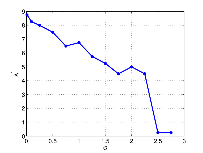
Experiment 1: We first consider recovering a signal vector from Gaussian measurements. We generate the measurement matrix $H^{n\times m}$ with i.i.d. ${N}(0,1)$ entries and a vector ${\mathbf{x}}^{\prime}\in{R}^{m}$ with i.i.d Gaussian entries. Let ${\mathbf{x}}={\mathbf{x}}^{\prime}/\|{\mathbf{x}}^{\prime}\|_{2}$ be the signal vector. Let $m=60$ and $n=150$. We first consider the recover performance when the number of erroneous measurements is fixed. We randomly choose twelve measurements and flip the signs of these measurements. For each measurement, we also independently add a Gaussian noise from ${N}(0,\sigma^{2})$. For a given $\sigma$, we apply (II.6) to estimate ${\mathbf{x}}$ using $\lambda$ from 0 to 13, and pick the best $\lambda^{*}$ with which the estimation error is minimized. For each $\sigma$, the result is averaged over fifty runs. Fig. 3 shows the curve of $\lambda^{*}$ against $\sigma$. When the number of measurements with bad data is fixed, $\lambda^{*}$ decreases as the noise level increases.

We next fix the noise level and consider the estimation performance when the number of erroneous measurements changes. Each measurement has a Gaussian noise independently drawn from ${N}(0,0.5^{2})$. Let $\rho$ denote the percentage of erroneous measurements. Given $\rho$, we randomly choose $\rho n$ measurements, and each such measurement is added with a Gaussian error independently drawn from ${N}(0,5^{2})$. The estimation result is averaged over fifty runs. Fig. 4 shows how the estimation error changes as $\rho$ increases for different $\lambda$. $\lambda=8$ has the best performance in this setup compared with a large value $\lambda=15$ and a small value $\lambda=0.05$.

Experiment 2: We also consider estimating the state of the power system from available measurements and known system configuration. The state variables are the voltage magnitudes and the voltage angles at each bus. The measurements can be the real and reactive power injections at each bus, and the real and reactive power flows on the lines. All the measurements are corrupted with noise, and a small fraction of the measurements contains errors. We would like to estimate the state variables from the corrupted measurements.

The relationship between the measurements and the state variables for a $k^{\prime}$-bus system can be stated as follows [12]:

where $P_{i}$ and $Q_{i}$ are the real and reactive power injection at bus $i$ respectively, $P_{ij}$ and $Q_{ij}$ are the real and reactive power flow from bus $i$ to bus $j$, $E_{i}$ and $\delta_{i}$ are the voltage magnitude and angle at bus $i$. $Y_{ij}$ and $\theta_{ij}$ are the magnitude and phase angle of admittance from bus $i$ to bus $j$, $Y_{si}$ and $\theta_{si}$ are the magnitude and angle of the shunt admittance of line at bus $i$. Given a power system, all $Y_{ij}$, $\theta_{ij}$, $Y_{si}$ and $\theta_{si}$ are known.

For a $k^{\prime}$-bus system, we treat one bus as the reference bus and set the voltage angle at the reference bus to be zero. There are $m=2k^{\prime}-1$ state variables with the first $k^{\prime}$ variables for the bus voltage magnitudes $E_{i}$ and the rest $k^{\prime}-1$ variables for the bus voltage angles $\theta_{i}$. Let ${\mathbf{x}}\in{R}^{m}$ denote the state variables and let ${\mathbf{y}}\in{R}^{n}$ denote the $n$ measurements of the real and reactive power injection and power flow. Let ${\mathbf{v}}\in{R}^{n}$ denote the noise and ${\mathbf{e}}\in{R}^{n}$ denote the sparse error vector. Then we can write the equations in a compact form,

where $h(\cdot)$ denotes $n$ nonlinear functions defined in (V.1) to (V.4).

An estimate of the state variables, $\hat{{\mathbf{x}}}$, can be obtained by solving the following minimization problem,

where $\hat{{\mathbf{x}}}$ is the optimal solution ${\mathbf{x}}$. $\lambda>0$ is a fixed parameter. When $\lambda\rightarrow\infty$, (V.6) approaches

and when $\lambda\rightarrow 0$, (V.6) approaches

Since $h$ is nonlinear, we linearize the equations and apply an iterative procedure to obtain a solution. We start with the initial state ${\mathbf{x}}^{0}$ where $x^{0}_{i}=1$ for all $i\in\{1,...,n\}$, and $x^{0}_{i}=0$ for all $i\in\{n+1,...,2n-1\}$. In the $k$th iteration, let $\Delta{\mathbf{y}}^{k}={\mathbf{y}}-h({\mathbf{x}}^{k-1})$, then we solve the following convex optimization problem,

where $H^{n\times m}$ is the Jacobian matrix of $h$ evaluated at ${\mathbf{x}}^{k-1}$. Let $\Delta{\mathbf{x}}^{k}$ denote the optimal solution $\Delta{\mathbf{x}}$ to (V.9), then the state estimation is updated by

We repeat the process until $\Delta{\mathbf{x}}^{k}\rightarrow 0$.

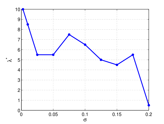
We evaluate the performance on the IEEE 30-bus test system. Fig. 5 shows the structure of the test system. Then the state vector contains fifty-nine variables. We take one hundred measurement including the real and reactive power injection at each bus and some of the real and reactive power flows on the lines. We first consider how the estimation performance changes as the noise level increases when the erroneous measurements are fixed. The errors of the measurements are simulated by inverting the sign of the real power injection at bus 2, bus 3, bus 5, bus 26 and bus 30, and inverting the sign of the reactive power injection at bus 30. Each measurement also contains a Gaussian noise independently drawn from ${N}(0,\sigma^{2})$. For a fixed noise level $\sigma$, we solve (V.6) by the iterative procedure using different $\lambda$ (from 0.5 to 12). The estimation performance is measured by $\|{\mathbf{x}}^{*}-\hat{{\mathbf{x}}}\|_{2}$, where ${\mathbf{x}}^{*}$ is the true state variable and $\hat{{\mathbf{x}}}$ is our estimation. For a fixed $\sigma$, we choose the $\lambda^{*}$ to be the one with which $\|{\mathbf{x}}^{*}-\hat{{\mathbf{x}}}\|_{2}$ is minimal among all the $\lambda$’s we consider. The result is averaged over fifty runs. Fig. 6 shows how $\lambda^{*}$ changes as $\sigma$ increases from 0 to 0.2. When the noise level is low, i.e. the measurements basically only contain errors, then the estimation performance is better when we use a larger $\lambda$. When the noise level is high, a smaller $\lambda$ leads to a better performance.

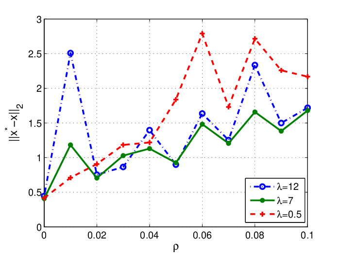
We also study how the estimation performance changes as the number of erroneous measurements increases. Each of the one hundred measurements contains random Gaussian noise independently drawn from ${N}(0,0.05^{2})$. Let $\rho$ denote the percentage of erroneous measurements with bad data. For fixed $\rho$, we randomly choose the set $T$ of erroneous measurements with cardinality $|T|=\rho m$. Each erroneous measurement contains an additional Gaussian error independently drawn from ${N}(0,0.7^{2})$. We than calculate the solution $\hat{{\mathbf{x}}}$ of (V.6) and the estimation error $\|{\mathbf{x}}^{*}-\hat{{\mathbf{x}}}\|_{2}$. Fig. 7 shows how the estimation error changes as $\rho$ increases. The results are averaged over fifty runs. When $\lambda$ is small ($\lambda=0.5$), (V.6) approaches (V.7), and the estimation error is relatively large if $\rho$ is small, i.e. the measurements basically contain only noise. When $\lambda$ is large ($\lambda=12$), (V.6) approaches (V.8), and the estimation error is relatively large if $\rho$ is large, i.e. the measurements contains errors besides noise. In contrast, if we choose $\lambda$ to be 7 in this case, the estimation error is relatively small for all $\rho$ among the three choices of $\lambda$.

In this paper, we study state estimation through observations corrupted with both bad data and additive observation noises. A mixed $\ell_{1}$ and $\ell_{2}$ convex programming is used to separate both sparse bad data and additive noises from the observations. We used the almost Euclidean property of a linear subspace to provide sharp bounds on this convex programming based state estimation method. We also give sharp bounds for the almost Euclidean property of a linear subspace using the “escape-through-a-mesh” theorem from geometric functional analysis [5]. We then propose an iterative convex programming based methods to perform state estimation with bad data detection in the nonlinear electrical power network problems. Simulation results confirm the effectiveness of the algorithms in denoising and detecting bad data at the same time.

The research is supported by NSF under CCF-0835706 and ONR under N00014-11-1-0131.

References

- [1] Anjan Bose and Kevin Clements, “Real-Time Modeling of Power Networks,” Proceedings of IEEE, 75(12), 1607-1622 1987
- [2] A. Monticelli and A. Garcia, “Reliable bad data processing for real time state estimation,” IEEE Trans. Power App. Syst., vol. PAS-102, pp.1126-1139, May 1983.
- [3] Broussolle, “State estimation in power systems: Detecting bad data through the sparse inverse matrix method,” IEEE Trans. Power App. Syst., vol. PAS-94, pp. 329-337, Mar./Apr. 1975.
- [4] Emmanuel Candès and Terence Tao, “Decoding by linear programming”, IEEE Trans. on Information Theory, 51(12), pp. 4203 - 4215, December 2005.
- [5] Y. Gordon, “On Milman’s inequality and random subspaces with escape through a mesh in ”, Geometric Aspect of Functional Analysis, Isr. Semin. 1986-87, Lect. Notes Math, 1317,1988.
- [6] M. Rudelson and R. Vershynin, “On sparse reconstruction from Fourier and Gaussian measurements”, Comm. on Pure and Applied Math., 61(8), 2007.
- [7] M. Stojnic, “Various thresholds for -optimization in Compressed Sensing,” http://arxiv.org/abs/0907.3666
- [8] S. Geman, “A limit theorem for the norm of random matrices,” Annals of Probability, vol. 8, No. 2, pp.252-261, 1980
- [9] J. Silverstein, “The smallest eigenvalue of a large dimensional Wishart matrix,” Annals of Probability, vol. 13, pp. 1364-1368, 1985
- [10] V. A. Marčenko and L. A. Pastur, “Distributions of eigenvalues for some sets of random matrices,” Math. USSR-Sbornik, vol. 1, pp. 457-483, 1967.
- [11] E. Candès and P. Randall, “Highly robust error correction by convex programming,” IEEE Transactions on Information Theory, vol. 54, pp. 2829-2840.
- [12] W. Kotiuga and M. Vidyasagar, “Bad Data Rejection Properties of Weighted Least Absolute Value Techniques Applied to Static State Estimation,” IEEE Trans. Power App. Syst., vol. PAS-101, pp. 844-853, Apr. 1982.
- [13] O. Kosut, L. Jia, R. J. Thomas, and L. Tong, ”On Malicious Data Attacks on Power System State Estimation,” Proceedings of UPEC,Cardiff, Wales, UK, 2010.
- [14] O. Kosut, L. Jia, R. J. Thomas, and L. Tong, “Malicious Data Attacks on Smart Grid State Estimation: Attack Strategies and Countermeasures” Proceedisng of IEEE 2010 SmartGridComm, 2010.
- [15] Yin Zhang, “A Simple Proof for Recoverability of -Minimization: Go Over or Under?” Technical Report, http://www.caam.rice.edu/ yzhang/reports/tr0509.pdf