LPT Orsay 11/37

Frozen shuffle update
for an asymmetric exclusion process
on a ring

C. Appert-Rolland, J. Cividini, and H.J. Hilhorst Affiliation: 2 - CNRS; UMR 8627; LPT Affiliation: Batiment 210, F-91405 ORSAY Cedex, France. Email: Cecile.Appert-Rolland@th.u-psud.fr Email: Henk.Hilhorst@th.u-psud.fr Email: ,

Abstract

We introduce a new rule of motion for a totally asymmetric exclusion process (TASEP) representing pedestrian traffic on a lattice. Its characteristic feature is that the positions of the pedestrians, modeled as hard-core particles, are updated in a fixed predefined order, determined by a phase attached to each of them. We investigate this model analytically and by Monte Carlo simulation on a one-dimensional lattice with periodic boundary conditions. At a critical value of the particle density a transition occurs from a phase with ‘free flow’ to one with ‘jammed flow’. We are able to analytically predict the current-density diagram for the infinite system and to find the scaling function that describes the finite size rounding at the transition point.

Keywords: pedestrian traffic, exclusion process, shuffle update, periodic boundary conditions

1 Introduction

L et a set of hard-core particles, labeled by an index $i=1,2,\ldots,N,$ move unidirectionally from site to site on a one-dimensional lattice. We imagine that the particles represent pedestrians all walking at the same pace but not necessarily in phase with each other. This leads us to formulate the following rule of motion, that we state as the update scheme of a Monte Carlo simulation. Each particle $i$ is assigned a phase $\tau_{i}\in[0,1)$ , permanently attached to it, and during each time step (that is, each unit time interval) all $N$ particles make a forward hopping attempt in the order of increasing phases. An attempted hop will succeed only if the target site is empty.

This model is an instance of what are commonly called Totally Asymmetric Simple Exclusion Processes (TASEP); its novelty resides in its update rule. Before continuing the discussion, we mention some connections to existing work.

Processes of particles moving stochastically on – often one-dimensional – lattices serve on the one hand as archetypes of out-of-equilibrium systems, and on the other hand as modeling tools to study transport in various systems, ranging from road and pedestrian traffic to intracellular traffic [1]. The particle motion may take place according to a large diversity of hopping rules. By the ‘exclusion’ principle one imposes the hard core condition (at most one particle per site); the ‘total asymmetry’ forbids backward hops; and the process is called ‘simple’ when hops are only between nearest-neighbor sites.

Given these three properties that are characteristic of a TASEP, it is still possible to choose from a variety of update schemes. In particular, the following update schemes have been studied: parallel update [2, 3, 4, 5], random sequential update, sequential update ordered backward or forward in space [6, 7, 8, 9, 3], sublattice update [10, 11, 12], and random shuffle update [13, 14]. The properties of the system depend on the update scheme [15] and the choice of the scheme should be determined by the application.

The most common update schemes are the random sequential and the parallel updates. Random sequential update produces a dynamics very close to that defined by a master equation in continuous time. A time step is defined as a succession of $N$ elementary updates, each associated with a time interval of length $1/N$ , and each allowing only a single particle, chosen at random, to make a hopping attempt. With this dynamics considerable fluctuations occur, since the same particle may be updated several times in the same time step whereas another one may be ignored during several time steps.

With parallel update particles make hopping attempts only at integer values of time but then do so simultaneously. Parallel update is used in particular for applications to road traffic [16, 17]: all vehicles are moving at the same time and the time step of the scheme is then supposed to represent a reaction time. Fluctuations are reduced, but parallel update can create conflicts – that should be settled by additional rules – when more than one particle tries to hop onto the same target site. This may occur in particular in applications to pedestrian traffic, which usually takes place in two-dimensional space.

In order to overcome the limitations of these two types of updates, the so-called ‘shuffle update’ has been proposed for modeling pedestrian flow. In the random shuffle update [13, 14], before each time step the particles are pre-arranged in a randomly chosen order and then each of them is updated once, exactly in that order. This update scheme was used for example in [18] for large-scale simulations of pedestrians.

In the present paper we explore a variant of the shuffle update for which the order in which the particles are arranged, that is, the updating order, is fixed once and for all¹¹ 1 This frozen variant was mentioned, but not studied, in the conclusion of [13].. Our scheme is therefore appropriately characterized by the name of ‘frozen shuffle update’.

For a closed system this is easy to implement; a random phase $\tau_{i}$ is drawn for each of the $N$ particles independently, for example from the uniform distribution on $[0,1)$ . In each time step all $N$ particle positions are updated once, one after the other, according to increasing values of their phases. The phases $\tau_{i}$ do not change during the whole simulation and may be considered as frozen variables of the motion. The set $\{\tau_{i}\}$ determines a random permutation of the particles; for uniformly distributed $\tau_{i}\,$ , all permutations have the same probability.

A closed system is expected to evolve towards a stationary state. We must be prepared to envisage that the final stationary state may depend (and as we shall see, indeed does depend) on the precise permutation that fixes the updating order of the particles. An average over all permutations is therefore appropriate and is analogous to the averages on quenched disorder variables standardly performed in statistical physics. The term ‘disorder average’ will therefore denote below the average over all random assignments $\{\tau_{i}\}$ .

For an open system the frozen shuffle update requires that by a suitable algorithm we fix the phase of each particle the moment it enters. The equivalence of the set $\{\tau_{i}\}$ to a simple permutation may then no longer hold. The case of open boundary conditions will not be considered here but is studied in a forthcoming paper [22].

In section 2 we introduce some terminology that actually already is the expression of several model properties. In section 3 we consider the TASEP with frozen shuffle update on a ring with particle density $\rho$ . We show that a phase transition occurs at a critical density $\rho_{\rm c}$ which separates a low density regime with ‘free flow’ from a high density regime with ‘jammed flow’. We determine the current-versus-density curve $J_{L}(\rho)$ analytically, first for an infinite system (section 3.1) where $J(\rho)=\lim_{L\to\infty}J_{L}(\rho)$ has a cusp, and then for a system of finite size $L$ (section 3.2), where the finite size rounding of $J_{L}(\rho)$ is described by a scaling function that depends only on the product variable $(\rho-\rho_{\rm c})L^{1/2}$ . Monte Carlo simulations show very good agreement with theory. In section 4, by way of a supplement, we show that under ‘free flow’ conditions the TASEP with frozen shuffle update is equivalent to a system of noninteracting particles in continuous space and time. In section 5 we conclude.

2 Free flow and jammed flow

We introduce here the concepts that characterize the structures formed by the particles as they result from the frozen shuffle update scheme. The discussion below is independent of any boundary conditions that may be imposed at a later stage. The most important point is the identification of two distinct stable flow states that we call the free flow state and the jammed state.

2.1 Well-ordered and ill-ordered pairs

Let the flow direction be to the right, let the particles be numbered $\ldots,i-1,i,i+1,\ldots$ from right to left (see figure 1), and let their phases $\ldots,\tau_{i-1},\tau_{i},\tau_{i+1},\ldots$ be given. The pair of successive particles $(i,i+1)$ , not necessarily on adjacent sites, will be called well-ordered if $\tau_{i+1}>\tau_{i}$ and ill-ordered in the opposite case. The time evolution of well- and ill-ordered pairs under the frozen shuffle update scheme has the following properties, illustrated in figure 1.

Refer to caption — Figure 1: Lattice sites are represented by squares that may be either empty or occupied by a single particle. A configuration involving four particles is shown at two successive times $t=s$ and $t=s+1$ ; the flow is in the direction of the arrow. Particles 1 and 2 form a well-ordered pair. They can move at the same time step, as particle 1 is updated before particle 2. Particles 3 and 4 form an ill-ordered pair. During the time step from $t=s$ to $t=s+1$ the update attempt of particle 4 is performed at time $s+\tau_{4}$ but remains unsuccessful, since its target site is still occupied by particle 3. When subsequently particle 3 is updated at time $s+\tau_{3}$ , it moves forward. Thus a hole is inserted between the two particles. In case $\tau_{3}<\tau_{2}$ , particles 2 and 3 also form an ill-ordered pair, but they are not adjacent and thus can hop independently.

If a well-ordered pair $(i,i+1)$ occupies two adjacent sites, then at each time step particle $i$ will move first and particle $i+1$ will move next; hence when the time step is completed, the two particles are still adjacent and have advanced one lattice distance to the right. Their speed is $v=1$ in units of lattice distances per time step.

If an ill-ordered pair occupies two adjacent sites, the two particles cannot move in the same time step; particle $i+1$ , having $\tau_{i+1}<\tau_{i}$ , will attempt first to move but finds itself blocked by particle $i$ . Hence the two particles of an ill-ordered pair move at speed $v=1$ only if they are separated by at least one empty site.

2.2 Free flow configuration

A particle configuration will be said to satisfy the free flow (FF) condition when each ill-ordered pair has its two members separated by at least one hole. In view of the above, such a configuration is again identical to itself at the end of each time step except for a translation by one lattice distance to the right. This corresponds to a free flow with speed $v=1$ , and hence for a FF configuration we have

J=\rho,

(1)

where $J$ is the current and $\rho$ the particle density. It is tacitly understood here that these quantities refer to time averages in a stationary state.

2.3 Rising sequences and platoons

Going along the lattice from right to left one may divide the particles encountered into sequences of increasing phases (for short: rising sequences). The set of particles $(i,i+1,\ldots,i^{\prime})$ will be said to constitute a rising sequence if $\tau_{i}<\tau_{i+1}<\ldots<\tau_{i^{\prime}}$ but $\tau_{i-1}>\tau_{i}$ and $\tau_{i^{\prime}}>\tau_{i^{\prime}+1}$ . Examples are shown in figure 2.

Let a set of particles occupy consecutive sites and have phases that increase from right to left. If this set corresponds to a full rising sequence, it will be called a platoon. If it corresponds to only part of a rising sequence, it will be called a subplatoon. One may say that a platoon (a subplatoon) is a fully compacted rising sequence (part of a rising sequence). Platoons and subplatoons are limited on both ends either by holes or by ill-ordered pairs. A rising sequence is composed either of a single platoon or of several subplatoons, an isolated particle being considered as a (sub-)platoon of length $1$ .

Under the frozen shuffle update platoons and subplatoons obey the following simple rules.

i(i) If in a given time step the first particle of a (sub-)platoon can move, then all its other particles will also move; hence (sub-)platoons move as single entities.

(ii) When two subplatoons merge, they can never separate again; hence the length of a subplatoon can only grow until it includes the whole rising sequence in which it is embedded.

2.4 Jammed configuration

A configuration of particles will be called jammed if all its rising sequences are compacted into platoons and if consecutive platoons are separated by at most one hole. Figure 3 shows an example of a jammed configuration. At each time step the evolution of a jammed configuration may be simply described in terms of the motion of its platoons. The rules follow directly from those above:

i(i) A platoon preceded by a hole advances by one site as a single entity; this amounts to a position exchange of the platoon and the hole.

(ii) A platoon not preceded by a hole is blocked and does not advance.

Let $\nu$ stand for the average platoon length in a jammed configuration that is statistically homogeneous in space. Noting that $1-\rho$ is the hole density and that only platoons preceded by a hole move, we may write the particle current in this jammed configuration as

J=(1-\rho)\nu.

(2)

Obviously, configuration space has many configurations that are neither ‘free flow’ nor ‘jammed’ in the sense of the above definitions. There is also one subclass of configurations that are both ‘free flow’ and ‘jammed’; this happens when all platoons of a jammed configuration are separated by exactly one hole.

3 Phase transition on a ring

After the preliminaries of section 2 we are now ready to study a concrete system. We consider a ring, that is, a lattice of $L$ sites with periodic boundary conditions. Let $N$ be the number of particles and hence $\rho=N/L$ the particle density. We set ourselves the purpose of determining the particle current $J_{L}(\rho)$ as a function of the particle density $\rho$ in the stationary state that will result from a given initial state.

At the initial time $t=0$ the particles are placed at distinct but otherwise random positions on the lattice. They are numbered $i=1,2,\ldots,N$ from right to left (clockwise around the lattice) and their direction of motion is from left to right (anticlockwise). The particles are assigned a random phases $\tau_{i}$ which we take independently and uniformly distributed on $[0,1)$ . This assignment determines the updating order of the particles.

The initial configuration does not necessarily satisfy the FF condition. If it does, then the particle configuration at time $t=s$ is obtained from that at time $t=0$ by rotating all particle positions by $s$ steps along the ring. If the FF condition is not satisfied, then after a transient period the system will reach a stationary state which may or may not be of the FF type. We will investigate below the conditions for the realization of each of these possibilities, and the ensuing consequences for the particle current.

3.1 Infinite system limit

The infinite system limit is easiest to discuss, since we may apply the law of large numbers and formulate statements that in that limit are true with probability 1. Let us first ask up to which value of the density $\rho$ it is still possible to have free flow.

For a given set $\{\tau_{i}\}$ the densest possible FF configuration occurs when all rising sequences are compacted into platoons separated by a single hole. This corresponds precisely to the aforementioned special case of a configuration which is both FF and jammed. The maximum density of the FF phase thus is $\rho_{\rm c}=\nu/(\nu+1)$ , where as before $\nu$ is the average platoon length. It may be shown (see [19] or Appendix A) that in the infinite system limit one has $\nu=2$ when the phases $\tau_{i}$ are uniformly distributed, and therefore $\rho_{\rm c}=\frac{2}{3}$ .

For $\rho\leq\rho_{\rm c}$ any arbitrary initial configuration – tacitly understood to be statistically homogeneous in space – will, after a transient, be converted into a FF configuration. Indeed, whenever an ill-ordered pair of particles occupies two successive sites, the second one will not yet be able to move when the first one first moves forward, and a hole will naturally be included between them. When in this way all ill-ordered pairs have come to include a hole, a FF configuration is obtained. The current $J(\rho)=\lim_{L\to\infty}J_{L}(\rho)$ is then given by its FF value (1),

J(\rho)=\rho,\qquad\rho\leq\rho_{\rm c}\,.

(3)

For $\rho>\rho_{\rm c}$ the time evolution will produce two effects. It will compact rising sequences into platoons and it will distribute the available holes such that each platoon is separated from its predecessor by at most a single hole. However, the number of holes is less than the number of platoons. The number of platoons that move in a given time step has thus been maximized and is equal to the number of holes, the other platoons being blocked at that time step. This corresponds to the definition of a jammed phase given in section 2.4, whence upon applying (2) with $\nu=2$ we obtain

J(\rho)=2(1-\rho),\qquad\rho\geq\rho_{\rm c}\,.

(4)

Equations (3) and (4) lead to the cusped current-density diagram shown in figure 4. The agreement with finite size Monte Carlo simulations is already quite good for system size $L=12$ . However, finite size effects are visible around the maximum, as shown in the inset of figure 4. In the next section we shall refine the theory to account for this rounding of the transition.

3.2 Finite system

We consider in this subsection a finite ring of size $L$ containing exactly $N$ particles; throughout we set $\rho=N/L$ . Our interest is in the density dependent particle current, which in this finite system we shall denote by $J_{L}(\rho)$ and whose definition we shall render precise.

By the mechanism described above the system, whatever its initial configuration, will evolve so as to maximize the number of ill-ordered pairs that include a hole. For densities $\rho\leq 1/2$ , there is enough space in the system to place a hole between each pair of particles. Then the FF condition can be fulfilled with certainty and the stationary state is a FF state. Denoting the current in the stationary state by $J_{NL}$ we have

J_{NL}=\frac{N}{L}=\rho,\qquad\rho\leq\mbox{$\frac{1}{2}$}.

(5)

For densities $\rho>1/2$ it may or may not be possible to converge towards an FF configuration, depending on the random assignment $\{\tau_{i}\}$ . The considerations of section 2.2 show that the discriminating quantity is the number of ill-ordered particle pairs in the initial state. We denote by $n^{\rm w}$ (by $n^{\rm i}$ ) the number of well-ordered (ill-ordered) pairs, so that $n^{\rm w}+n^{\rm i}=N$ . It will be convenient to work with the difference variable

n\big(\{\tau_{i}\}\big)=n^{\rm w}-n^{\rm i}\,,

(6)

of which we shall henceforth suppress the argument. Because of the periodic boundary conditions, there is always at least one ill-ordered pair and one well-ordered pair in the system, so that $n$ may take the values $n=1,2,\ldots,N-1$ . A necessary and sufficient condition to fulfill the FF condition in the stationary state is to have at least one empty site available for each ill-ordered pair, that is, $n^{\rm w}+2n^{\rm i}\leq L$ or equivalently

n\geq\mbox{$\frac{3}{2}$}N-L.

(7)

The expression for the stationary state current now involves the variable $n$ and we will denote it by $J_{NLn}$ . Two cases have to be distinguished. First, if inequality (7) is satisfied, the system evolves towards a FF state and for this subset of realizations the current is

J_{NLn}=\frac{N}{L}=\rho,\qquad\rho>\mbox{$\frac{1}{2}$}\,,\quad\frac{n}{N}\geq\mbox{$\frac{3}{2}$}-\rho^{-1}\,.

(8)

Secondly, we consider realizations $\{\tau_{i}\}$ for which inequality (7) is violated. The stationary state then only has isolated holes²² 2 The same behavior appears with random shuffle update., and all rising sequences are compacted into platoons. At each time step only the platoons headed by one of the $L-N$ holes move forward, which means that the instantaneous current per time step fluctuates with time. However, averaged over time each platoon will move in a fraction $(L-N)/N$ of all time steps. Using the fact that ${N}/{n^{\rm i}}=2/(1-n/N)$ is the average length of a platoon, we therefore find after time averaging for the current $J_{NLn}$ the expression

J_{NLn}=\frac{L-N}{L}\times\frac{N}{n^{\rm i}}=\frac{2(1-N/L)}{1-n/N},\qquad\rho>\mbox{$\frac{1}{2}$}\,,\quad\frac{n}{N}<\mbox{$\frac{3}{2}$}-\rho^{-1}.

(9)

For finite systems and for densities $\frac{1}{2}<\rho<1$ , there will always exist realizations of the $\tau_{i}$ that converge towards FF stationary states with a current $\rho$ , and others that do not and have a current less than $\rho$ and given by (9). In this density regime we will denote by $J_{NL}$ the current $J_{NLn}$ of (8) and (9) averaged with respect to $n$ , that is,

J_{NL}=\sum_{n=1}^{N-1}P_{N}(n)J_{NLn}\,,\qquad\rho>\mbox{$\frac{1}{2}$}\,,

(10)

in which $P_{N}(n)$ is the probability distribution of $n\big(\{\tau_{i}\}\big)$ and remains to be determined. Since $n$ is determined by $\{\tau_{i}\}$ , the current $J_{NL}$ in (10) deserves the name of ‘disorder averaged current’.

3.3 Finite size effects near the transition point

The probability distribution $P_{N}(n)$ was studied by Oshanin and Voituriez [19] for the case – which is also ours – where the $\tau_{i}$ are drawn independently from a uniform distribution on $[0,1)$ . These authors showed, among other things, that in the limit of large $N$ and with $n$ scaling as $\sim N^{1/2}$ the variable $x=n/N^{1/2}$ has the probability distribution

\Pi(x)=(3/2\pi)^{1/2}\exp\left(-\mbox{$\frac{3}{2}$}x^{2}\right).

(11)

It is symmetric in $n$ , as dictated by the left-right symmetry of the phase assignment. In Appendix A we derive equation (11) in a more direct way.

From here on we shall consider the equations of the preceding subsection in the limit of large but finite $N$ , $n$ and $L$ , and fixed ratios $\rho=N/L$ and $x=n/N^{1/2}$ . We will conform to usage and take the system size $L$ , rather than $N$ , as the independent large variable. In the limit in question we shall write $J_{NLn}=J_{L}(\rho,x)$ and $J_{NL}=J_{L}(\rho)$ . We may then reexpress the disorder averaged current (10) as

J_{L}(\rho)=\int_{-\infty}^{\infty}\!{\rm d}x\,\Pi(x)J_{L}(\rho,x).

(12)

The expression for $J_{L}(\rho,x)$ is derived from (8) or (9), depending on the value of $x$ , that is,

J_{L}(\rho,x)=\left\{\begin{array}[]{ll}\frac{2(1-\rho)}{1-x(\rho L)^{-1/2}},&x<x_{\rm c}(\rho),\\[5.69054pt] \rho,&x\geq x_{\rm c}(\rho),\end{array}\right.

(13)

in which

x_{\rm c}(\rho)=(\rho L)^{1/2}\left(\rho_{\rm c}^{-1}-{\rho}^{-1}\right)

(14)

where $\rho_{\rm c}=\frac{2}{3}$ . We observe parenthetically that in the limit $L\to\infty$ the $x$ dependence of (14) disappears and we recover $\lim_{L\to\infty}J_{L}(x,\rho)=J(\rho)$ , where $J(\rho)$ is the infinite system current of equations (3) and (4). Since (11) is valid in the limit in which $x$ remains finite as $L\to\infty$ , we conclude that the present approach is valid for densities

\rho=\rho_{\rm c}+\Delta\rho

(15)

such that $\Delta\rho$ is on the scale of $L^{-1/2}$ . Remembering this and expanding in powers of $L^{-1/2}$ we find from (14) and (13)

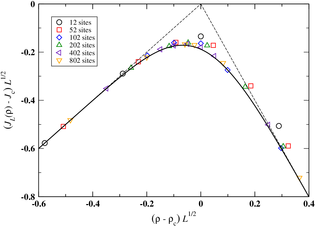
	$\displaystyle x_{\rm c}(\rho)$	$\displaystyle=$	$\displaystyle(\mbox{$\frac{3}{2}$})^{3/2}L^{1/2}\Delta\rho+{\cal O}(L^{-1/2}),$
	$\displaystyle J_{L}(\rho,x)$	$\displaystyle=$	$\displaystyle\left\{\begin{array}[]{ll}\rho_{\rm c}-2\Delta\rho+(3L/2)^{-1/2}x+{\cal O}(L^{-1}),&x<x_{\rm c}(\rho),\\[5.69054pt] \rho_{\rm c}+\Delta\rho,&x\geq x_{\rm c}(\rho).\end{array}\right.$

We introduce the scaling variable $y=L^{1/2}\Delta\rho$ , which in the limit of interest should be of order unity. Substitution of (3.3) in (12) then yields

J_{L}(\rho)=\rho_{\rm c}+L^{-1/2}y-L^{-1/2}\int_{-\infty}^{(3/2)^{3/2}y}\!{\rm d}x\,\Pi(x)\left[3y-(\mbox{$\frac{2}{3}$})^{1/2}x\right]+{\cal O}(L^{-1}).

(19)

When using in (19) the explicit expression (11) for $\Pi(x)$ we may evaluate the $x$ integral and obtain, up to corrections of higher order in $L^{-1/2}$ ,

J_{L}(\rho)=\rho_{\rm c}+L^{-1/2}\Phi(L^{1/2}\Delta\rho),

(20)

valid in the limits $\Delta\rho=\rho-\rho_{\rm c}\to 0$ and $L\to\infty$ with $L^{1/2}\Delta\rho$ fixed, and in which the scaling function $\Phi(y)$ is given by

\Phi(y)=-\mbox{$\frac{1}{2}$}y-\mbox{$\frac{3}{2}$}y\,{\rm erf}\left(\mbox{$\frac{9}{2}$}y\right)-(9\pi)^{-1/2}\exp\left(-\mbox{$\frac{81}{4}$}y^{2}\right).

(21)

This function is negative and such that

	$\displaystyle\Phi(y)$	$\displaystyle\simeq$	$\displaystyle y,\phantom{\Delta\rho}\qquad y\to-\infty,$
	$\displaystyle\Phi(y)$	$\displaystyle\simeq$	$\displaystyle-2y,\qquad y\to\infty,$		(22)

which ensures the correct limit behavior of (20) for $|\rho-\rho_{\rm c}|\gg L^{-1/2}$ . We have plotted $\Phi(y)$ in figure 5 together with simulation data for different system sizes $L$ . The data are seen to collapse very well onto the theoretical curve.

4 Mapping to a continuous model and interpretation for pedestrian motion

In this section we point out that under free flow conditions the time evolution defined by the frozen shuffle update for the particle system on a lattice may be seen as a sequence of snapshots taken at integer instants of time $t=\ldots,s-1,s,s+1,\ldots$ , of a system that itself evolves in continuous time $t$ and space $x$ .

To show this we consider a collection of nonoverlapping hard rods all moving continuously to the right at speed $v=1$ along the $x$ axis, as depicted in figure 6. If we associate lattice sites with the integer axis positions $x=\ldots,k-1,k,k+1,\ldots$ , then at any given instant of continuous time, each rod covers exactly one site. The mapping is performed by placing on that site a particle associated with that rod. Let figure 6 represent the rod positions at time $t=0$ (or for that matter at any other integer instant of time). The particle labeled $i$ and corresponding to rod $i$ occupies lattice site $k$ and therefore gives rise, at $t=0$ , to a particle on site $k$ . The distance between site $k$ and the tail of rod $i$ has been indicated as a time interval³³ 3 Because $v=1$ , times and distances may be identified. $\tau_{i}$ , this being the time still needed for the tail of that rod to cross the point $k$ during its continuous motion along the $x$ axis. This crossing therefore occurs at time $t=\tau_{i}$ , and that is the time at which particle $i$ will hop from site $k$ to site $k+1$ . Particle $i$ will execute its subsequent hops at times $t=s+\tau_{i}$ , where $s$ is an integer. This is exactly the frozen shuffle update scheme.

We remark that the mapping defined here yields only the FF configurations of the discrete model. If we try to perform the inverse mapping, i.e. from the discrete to the continuous model, then in case of a jammed configuration the non-overlapping condition for rods cannot be enforced anymore. This may actually still have some physical relevance, if one adopts the view that a rod represents not only a pedestrian but also some “private” space around him. In free flow pedestrians are not willing to approach each other too closely and they avoid to enter each other’s “private” space, whereas at increasing densities they tolerate smaller distances.

5 Conclusion

We have introduced in this paper a new update scheme for the TASEP, namely the frozen shuffle update, which should be appropriate, in particular, for the modeling of pedestrians.

We have characterized the behavior of the TASEP with frozen shuffle update for a closed one-dimensional lattice of $L$ sites and $N$ particles. The time evolution under frozen shuffle update is deterministic⁴⁴ 4 By this we mean that the hopping probability is always unity when the target site is empty.; it is fully determined by the initial particle positions and by the set $\{\tau_{i}\}$ of their phases. The latter are quenched random variables that at each time step determine the update order of the particles. We showed that the analysis of the particle motion and their interaction may be fruitfully carried out in terms of the concepts of well/ill-ordered pairs and of platoons. Two principal types of flow may then be distinguished, ‘free flow’ and ‘jammed flow’.

We were able to predict completely the fundamental diagram, that is, the current $J_{L}(\rho)$ as a function of density $\rho=N/L$ , both for the infinite ( $N,L\to\infty$ ) and the finite system.

We found that for increasing particle density $\rho$ the passage from a free flow phase to a jammed phase takes place via a phase transition at a critical density $\rho=\rho_{\rm c}$ . This contrasts with the random sequential update, for which with increasing density the system becomes gradually more and more congested. Critical points, however, were observed in the fundamental diagram in other instances of deterministic motion, namely with parallel update [20, 21] and with random shuffle update [13, 14]. In the latter case, although the particle-hole symmetry is broken, the critical point was still found at the symmetric point $\rho_{c}=1/2$ ; by contrast, for the present frozen shuffle update we find $\rho_{c}=2/3$ , i.e. the asymmetry between holes and particles is still enhanced. Another difference is that for the random shuffle update the critical point is already present in finite systems, whereas for the frozen shuffle update the transition is rounded and becomes sharp only in the limit of infinite system size.

A mapping with a continuous model of hard rods is proposed, which is exact for free flow configurations, and may be useful for the interpretation of the results in terms of pedestrian motion.

Two final remarks about open questions are in place here. First, the deterministic time evolution studied in this paper entails that, if the target site is empty, particles hop with probability $p=1$ . Whereas in the case of a random sequential update the hopping probability $p$ can be modified through a simple rescaling of time, here such a rescaling is not possible. We therefore expect a qualitatively different behavior of the current $J(\rho)$ when the hopping probability $p$ is strictly less than one. We leave the analysis of this case for future work.

Second, this work has been exclusively concerned with a closed system. New types of questions arise when one applies frozen shuffle update to open systems. In a companion paper [22] we shall address the case of open boundary conditions and determine in particular the phase diagram.

Appendix A Random walk generated by a random permutation of $N$ integers

We arrange the integers $1,2,3,\ldots,N$ on the sites of a circular lattice and permute them randomly, all permutations having the same probability. Suppose that when going clockwise along the lattice in $N$ steps, we encounter $n^{\rm w}$ well-ordered and $n^{\rm i}$ ill-ordered pairs in the sense of section 2.1. Obviously $n^{\rm w}$ and $n^{\rm i}$ are random integers that depend on the permutation, and are such that $n^{\rm w}+n^{\rm i}=N$ . Let $n=n^{\rm w}-n^{\rm i}$ . We ask what the probability distribution $P_{N}(n)$ of $n$ is in the limit of large $N$ .

This question was first asked by Oshanin and Voituriez [19], who obtained the distribution $\Pi(x)$ given in (11). It is possible to arrive at same result in a different and, we believe, simpler way that we present here. It is based on establishing a recursion in $N$ . Suppose that the integers $1,2,\ldots,N$ have been permuted and placed on the sites of a circular $N$ -site lattice. A permutation of $1,2,\ldots,N+1$ on an $(N+1)$ -site lattice is obtained by inserting between two randomly chosen neighboring sites a new site carrying the integer $N+1$ . The probability $p_{N}^{\rm w}$ (or $p_{N}^{\rm i}$ ) to perform the insertion on a well-ordered (or on an ill-ordered) pair is

p_{N}^{\rm w,i}(n)=\mbox{$\frac{1}{2}$}[1\pm n/N].

(23)

In either case the original pair disappears and, since the newly inserted integer $N+1$ is necessarily larger than its two neighbors, is replaced with the succession of a well- and an ill-ordered pair. Hence we have the recursion

P_{N+1}(n)=p_{N}^{\rm w}(n-1)P_{N}(n-1)+p_{N}^{\rm i}(n+1)P_{N}(n+1),

(24)

valid for $n=-N+1,-N+3,\ldots,N-1$ (which are the only values of $n$ that can occur) and with the convention that $P_{N}(-N)=P_{N}(N)=0$ . We substitute (23) in (24) and set

x=\frac{n}{N^{1/2}}\,,\qquad P_{N}(n)=\frac{1}{N^{1/2}}\,\Pi_{N}\left(\frac{n}{N^{1/2}}\right),

(25)

expecting that in the large- $N$ limit the variables $x$ and $N$ may be treated as continuous. On the expression thus obtained we perform a standard expansion in negative powers of $N$ . The result is the Fokker-Planck equation

\frac{\partial\,\Pi_{N}(x)}{\partial N}=\frac{3}{2}\frac{\partial\,x\Pi_{N}(x)}{\partial x}+\frac{1}{2}\frac{\partial^{2}\,\Pi_{N}(x)}{\partial x^{2}}\,,

(26)

of which (11) is the stationary solution, that is, the one solving $\partial\,\Pi_{N}(x)/\partial N=0$ .

We also note that the average length of the platoons

\nu=\frac{N}{n^{\rm i}}=\frac{2N}{N-n}

(27)

tends to $\nu=2$ when $N$ becomes large, as $n$ typically scales as $N^{1/2}$ .

References

[1] D. Chowdhury, A. Schadschneider, and K. Nishinari. Physics of transport and traffic phenomena in biology: from molecular motors and cells to organisms. Physics of Life Reviews, 2:318–352, 2005.
[2] H. Hinrichsen. Matrix product ground states for exclusion processes with parallel dynamics. J. Phys. A: Math. Gen., 29:3659–3667, 1996.
[3] M.R. Evans. Exact steady states of disordered hopping particle models with parallel and ordered sequential dynamics. J. Phys. A: Math. Gen., 30:5669–5685, 1997.
[4] A. Schadschneider and M. Schreckenberg. Garden of Eden states in traffic models. J. Phys. A: Math. Gen., 31:L225–L231, 1998.
[5] M. Wölki and M. Schreckenberg. Exact matrix-product states for parallel dynamics: open boundaries and excess mass on the ring. J. Stat. Mech., P05014, 2009.
[6] A. Borodin, P.L. Ferrari, and M. Prahofer. Fluctuations in the discrete TASEP with periodic initial configurations and the Airy process. International Mathematics Research Papers, rpm002, 2007.
[7] J.G. Brankov, V.B. Priezzhev, and R.V. Shelest. Generalized determinant solution of the discrete-time totally asymmetric exclusion process and zero-range process. Phys. Rev. E, 69:066136, 2004.
[8] J.G. Brankov, V.V. Papoyan, V.S. Poghosyan, and V.B. Priezzhev. The totally asymmetric exclusion process on a ring: Exact relaxation dynamics and associated model of clustering transition. Physica A, 368:471–480, 2006.
[9] V.S. Poghosyan and V.B. Priezzhev. The relaxation dynamics of the TASEP with particle-dependent hopping probabilities on a ring. Reports on Mathematical Physics, 61:239–246, 2008.
[10] V. Fayaz, F.H. Jafarpour, S.R. Masharian, and S. Zeraati. One-transit paths and the steady state of a non-equilibrium process in a discrete-time update. J. Stat. Mech., P12009, 2010.
[11] C. Pigorsch and G.M. Schütz. Shocks in the asymmetric simple exclusion process in a discrete-time update. J. Phys. A: Math. Gen., 33:7919–7933, 2000.
[12] S.S. Poghosyan, V.B. Priezzhev, and G.M. Schutz. Green functions for the TASEP with sublattice parallel update. J. Stat. Mech., P04022, 2010.
[13] M. Wölki, A. Schadschneider, and M. Schreckenberg. Asymmetric exclusion processes with shuffled dynamics. J. Phys. A: Math. Gen., 39:33–44, 2006.
[14] D.A. Smith and R.E. Wilson. Dynamical pair approximation for cellular automata with shuffle update. J. Phys. A: Math. Theor., 40(11):2651–2664, 2007.
[15] N. Rajewsky, L. Santen, A. Schadschneider, and M. Schreckenberg. The asymmetric exclusion process: Comparison of update procedures. J. Stat. Phys., 92:151–194, 1998.
[16] K. Nagel and M. Schreckenberg. A cellular automaton model for freeway traffic. J. Phys. I, 2:2221–2229, 1992.
[17] C. Appert and L. Santen. Boundary induced phase transitions in driven lattice gases with meta-stable states. Phys. Rev. Lett., 86:2498–2501, 2001.
[18] H. Klüpfel. The simulation of crowds at very large events. In A. Schadschneider, T. Poschel, R. Kuhne, M. Schreckenberg, and D.E. Wolf, editors, Traffic and Granular Flow ’05, pages 341–346, 2007.
[19] G. Oshanin and R. Voituriez. Random walk generated by random permutations of $\{1,2,3,\ldots,n+1\}$ . J. Phys. A: Math. Gen., 37:6221–6241, 2004.
[20] A. Schadschneider and M. Schreckenberg. Cellular automaton models and traffic flow. J. Phys. A: Math. Gen., 26:L679–683, 1993.
[21] B. Eisenblätter, L. Santen, A. Schadschneider, and M. Schreckenberg. Jamming transition in a cellular automaton model for traffic flow. Phys. Rev. E, 57:1309–1314, 1998.
[22] C. Appert-Rolland, J. Cividini, and H.J. Hilhorst. Frozen shuffle update for an asymmetric exclusion process with open boundary conditions. Preprint, 2011.

Frozen shuffle update for an asymmetric exclusion process on a ring