Dynamic Interference Mitigation for Generalized Partially Connected Quasi-static MIMO Interference Channel

Liangzhong Ruan, Vincent K.N. Lau Affiliation: Dept. of Electronic and Computer Engineering
the Hong Kong University of Science and Technology
Email:

\{

stevenr, eeknlau

\}

@ust.hk

Abstract

Recent works on MIMO interference channels have shown that interference alignment can significantly increase the achievable degrees of freedom (DoF) of the network. However, most of these works have assumed a fully connected interference graph. In this paper, we investigate how the partial connectivity can be exploited to enhance system performance in MIMO interference networks. We propose a novel interference mitigation scheme which introduces constraints for the signal subspaces of the precoders and decorrelators to mitigate “many” interference nulling constraints at a cost of “little” freedoms in precoder and decorrelator design so as to extend the feasibility region of the interference alignment scheme. Our analysis shows that the proposed algorithm can significantly increase system DoF in symmetric partially connected MIMO interference networks. We also compare the performance of the proposed scheme with various baselines and show via simulations that the proposed algorithms could achieve significant gain in the system performance of randomly connected interference networks.

I Introduction

Recently, there is an intense research interest in the area of interference channels and the interference mitigation techniques. Interference alignment (IA) was proposed in [1, 2] to reduce the effect of multi-user interference and is extended to deal with interference in MIMO X-channels [3] and $K$ pairs interference channels [4]. The key idea of IA is to reduce the dimension of the aggregated interference by aligning interference from different transmitters into a lower dimension subspace at each receiver. Using infinite dimension extension on the time dimension (time selective fading), it is shown that the IA could achieve the optimal Degrees-of-Freedom (DoF) of $\frac{KN}{2}$ in $K$ -pair MIMO ergodic interference channels [4] with $N$ antennas at each node. In [5], the authors proposed the concept of ergodic alignment, which also utilizes symbol extension exploiting time-selective fading of interference channels.

One important challenge of IA scheme is the feasibility condition. For instance, the IA schemes in [4] requires $\mathcal{O}((KN)^{2K^{2}N^{2}})$ dimensions of signal space to achieve the $\frac{KN}{2}$ total DoF. To avoid such huge dimensions of signal space, some researchers have studied IA designs for quasi-static MIMO interference channels. With limited signal space dimensions, the achievable DoF of each transmitter-receiver pair in MIMO interference channels is upper bounded by $\frac{N_{t}+N_{r}}{K+1}$ (where $K$ is the number of transmitter-receiver pairs, $N_{t}$ , $N_{r}$ are the number of antennas at each transmitter and receiver, respectively) [6]. Unlike the time-selective or frequency-selective MIMO interference channels, total DoF of quasi-static MIMO interference channel does not scale with $K$ . Furthermore, it is quite challenging to design precoders and decorrelators that satisfy the IA requirements in limited dimension MIMO interference channels due to the feasibility problems [6]. In [7], an iterative precoders and decorrelators design based on alternating optimization is proposed for quasi-static MIMO interference channels. In [8, 9], some constructive methods to design precoders and decorrelators are proposed, but these schemes can only achieve 1 DoF per transmitter.

In fact, the technical challenge on the feasibility issue in limited dimension MIMO interference channels is highly related to the full connectivity in the interference graph. In practice, the interference channels are usually partially connected due to path loss, shadowing as well as spatial correlation. Most of the existing literatures have assumed fully connected MIMO interference channels such as equal path loss and spatially uncorrelated MIMO channels. Intuitively, partial connectivity may contribute to limiting the aggregate interference and this may translate into DoF gains in the system. In this paper, we are interested to study the potential benefit of partially connectivity in a $K$ -pair MIMO interference network with quasi static fading. There are several important technical challenges involved.

•

How to exploit partial connections in interference mitigation? Traditionally, it is well-known that partial connection (due to path loss, shadowing or spatial correlation) is detrimental to point-to-point MIMO performance [10, 11] because it reduces the number of spatial channels in the MIMO link. However, in MIMO interference channels, partial connection may also reduce the dimension of the undesired signals (the interference), leading to possible performance improvement. In other words, we can potentially design precoders to exploit the partial connection property and reduce the interference dimensions to other users.
•

Achievable DoF for partially connected MIMO interference channels. In order to obtain insights on the potential benefits or degradations of partial connections in MIMO interference channels, one would be interested in deriving DoF bounds. Existing DoF analysis of interference channels [4, 6] assumed i.i.d. MIMO fading channels (fully connected MIMO interference channels) and it is interesting to find out how the partial connection parameters such as node density and spatial correlation level affect total DoF of the system.

In this paper, we propose a novel two-stage dynamic interference mitigation scheme to exploit the potential benefit of general partial connections in limited dimension MIMO interference channels so as to improve the network total DoF. The proposed dynamic interference mitigation solution has two stages. The first stage determines the stream assignment and the subspace constraints for the precoders and the decorrelators based on the partially connected topology such as the path loss, shadowing and spatial correlation. The second stage determines the precoders and the decorrelators (based on the instantaneous channel state information) over the subspaces obtained from the first stage. Based on the proposed dynamic interference mitigation scheme, we shall derive an achievable DoF bound of a symmetric interference network and show that the DoF in partially connected MIMO interference channels can exceed the well-known DoF results of $\frac{N_{t}+N_{r}}{K+1}$ for i.i.d. MIMO interference channels. Furthermore, we shall discuss how the DoF gain is affected by the partial connectivity (path loss and spatial correlation) in the system. Finally, we shall compare the performance of the proposed scheme with various conventional baselines, and it can be observed that the proposed scheme offers significant performance gain over a wide range of system operating regimes.

II System Model

II-A General $K$ -pair Partially Connected Quasi-static MIMO Interference Channels

We consider a MIMO system with $K$ transmitter (Tx) and receiver (Rx) pairs. Each transmitter and each receiver has $N_{t}$ and $N_{r}$ antennas, respectively. Denote the channel fading coefficients from the Tx $n$ to the Rx $m$ as $\mathbf{H}_{mn}\in\mathbb{C}^{N_{r}\times N_{t}}$ . Let $d_{m}$ ( $\leq\min(N_{t},N_{r})$ ) be the number of data streams (DoF) transmitted by Tx-Rx pair $m$ . The received signal $\mathbf{y}_{m}\in\mathbb{C}^{d_{m}}$ at Rx $m$ is given by:

\displaystyle\mathbf{y}_{m}=\mathbf{U}_{m}\left(\mathbf{H}_{mm}\mathbf{V}_{m}\mathbf{x}_{m}+\sum_{n\neq m\in\{1,2,...,K\}}\mathbf{H}_{mn}\mathbf{V}_{n}\mathbf{x}_{n}+\mathbf{z}\right)

(1)

where $\mathbf{x}_{m}\in\mathbb{C}^{d_{m}}$ is the encoded information symbol for Rx $m$ , $\mathbf{U}_{m}\in\mathbb{C}^{d_{m}\times N_{r}}$ is the decorrelator of Rx $m$ , and $\mathbf{V}_{m}\in\mathbb{C}^{N_{t}\times d_{m}}$ is the transmit precoding matrix at the Tx $m$ . $\mathbf{z}\in\mathbb{C}^{N_{r}\times 1}$ is the white Gaussian noise with unit variance. The transmit power at the Tx $n$ is $\mathbb{E}(||\mathbf{V}_{n}\mathbf{x}_{n}||^{2})=P_{n}$ . The channel connectivity of the $K$ -pair interference channels $\{\mathbf{H}_{mn}\}$ is specified by the following model.

Assumption II.1 (General Partially Connected Model)

The elements of the channel states matrices $\{\mathbf{H}_{mn}\in\mathbb{C}^{N_{r}\times N_{t}}\}$ , $n,m\in\{1,2,...,K\}$ are random variables following certain distribution and have the following properties:

•

Independence: Random matrices $\{\mathbf{H}_{mn}\}$ $n,m\in\{1,2,...,K\}$ are mutually independent.
•

Partial Connectivity at the Transmitter Side: Define the Tx side partial connectivity as the null space of $\mathbf{H}_{mn}$ , e.g: $\mathcal{N}(\mathbf{H}_{mn})=\{\mathbf{v}\in\mathbb{C}^{N_{t}\times 1}:\mathbf{H}_{mn}\mathbf{v}=\mathbf{0}\}$ .
•

Partial Connectivity at the Receiver Side: Define the Rx side partial connectivity as the “transposed” null space of $\mathbf{H}_{mn}$ , e.g: $\mathcal{N}^{H}(\mathbf{H}_{mn})=\{\mathbf{u}\in\mathbb{C}^{1\times N_{r}}:\mathbf{H}^{H}_{mn}\mathbf{u}^{H}=\mathbf{0}\}=\{\mathbf{u}\in\mathbb{C}^{1\times N_{r}}:\mathbf{u}\mathbf{H}_{mn}=\mathbf{0}\}$ . ∎

As a result, $\{\mathcal{N}(\mathbf{H}_{mn})\}$ and $\{\mathcal{N}^{H}(\mathbf{H}_{mn})\}$ $m,n\in\{1,2,...,K\}$ are the connection topological parameters of the general partially connected model. This is a general model as no specific structure is imposed on $\{\mathcal{N}(\mathbf{H}_{mn})\}$ and $\{\mathcal{N}^{H}(\mathbf{H}_{mn})\}$ . To help readers get some concrete understanding on the physical scenarios when we have partial connectivity, we shall illustrate some examples of partially connected interference channels in the next section. Note that the partial connectivity model imposed in Assumption II.1 contains, but is not limited to, these examples.

II-B Example Scenarios of Partially Connected Systems

II-B1 Path Loss and Shadowing

In practice, different Txs may contribute differently to the aggregate interference due to the heterogeneous path loss and shadowing effects. For example, in a $K$ -pair MIMO interference network with $N_{t}=N_{r}$ , suppose some Txs and Rxs are far away from each other when the difference between their node indices $|n-m|>L$ , the path loss and shadowing from Tx $n$ to Rx $m$ , is 60 dB higher than that of the direct link (from Tx $n$ to Rx $n$ , $n\in\{1,2,...,K\}$ ) and hence, effectively, we have $\mathbf{H}_{mn}=\mathbf{0}$ , $\forall|n-m|>L$ . This corresponds to a partially connected MIMO interference channel (induced by path loss and shadowing effects) with the connection topology given by $\mathcal{N}(\mathbf{H}_{mn})=\left\{\begin{array}[]{l}\mathbb{C}^{N_{t}\times 1}\mbox{ if }|n-m|>L\\ \{0\}\mbox{ otherwise}\end{array}\right.$ , $\mathcal{N}^{H}(\mathbf{H}_{mn})=\left\{\begin{array}[]{l}\mathbb{C}^{1\times N_{r}}\mbox{ if }|n-m|>L\\ \{0\}\mbox{ otherwise}\end{array}\right.$ .

II-B2 Unequal Transmit and Receive Antennas

When $N_{t}\neq N_{r}$ , there is a rank $|N_{t}-N_{r}|$ null space on the side with more antennas. For example, when $N_{t}=4$ , $N_{r}=2$ , denote $\mathbf{H}_{mn}=\left[\begin{array}[]{c}\mathbf{h}_{mn}(1)\\ \mathbf{h}_{mn}(2)\end{array}\right]$ , where $\mathbf{h}_{mn}(p)$ are $1\times 4$ vectors. Hence, this corresponds to a partially connected MIMO interference channel (induced by non-square fading matrices) with the connection topology given by: $\mathcal{N}(\mathbf{H}_{mn})=(\mbox{span}(\mathbf{h}^{T}_{mn}(1),\mathbf{h}^{T}_{mn}(2)))^{\bot}$ , $\mathcal{N}^{H}(\mathbf{H}_{mn})=\{0\}$ , $\forall m,n\in\{1,2,...,K\}$ .

II-B3 Spatial Correlation

As shown in [12],[13], in practice, local scattering effect causes significant spatial correlation in MISO channels. To explore the similar effect in MIMO channels and get a direct association between the MIMO fading channel correlation and the physical scattering environment, we shall introduce the virtual angular domain representation for MIMO channels [11]. Specifically, the MIMO fading channels in the antenna domain $\mathbf{H}_{mn}^{ant}$ and in the angular domain $\mathbf{H}_{mn}^{ang}$ have a one-one correspondence given by:

\displaystyle\mathbf{H}^{ant}_{mn}=\mathbf{A}_{R}\mathbf{H}^{ang}_{mn}\mathbf{A}^{H}_{T}

(2)

$\displaystyle\mbox{where: }\;\;\;\mathbf{A}_{T}$	$\displaystyle=$	$\displaystyle[\mathbf{e}_{N_{t}}(0),\mathbf{e}_{N_{t}}\left(\frac{1}{N_{t}}\right)...,\mathbf{e}_{N_{t}}\left(\frac{N_{t}-1}{N_{t}}\right)]$	(3)
$\displaystyle\mathbf{A}_{R}$	$\displaystyle=$	$\displaystyle[\mathbf{e}_{N_{r}}(0),\mathbf{e}_{N_{r}}\left(\frac{1}{N_{r}}\right)...,\mathbf{e}_{N_{r}}\left(\frac{N_{r}-1}{N_{r}}\right)]$	(4)
$\displaystyle\mathbf{e}_{N}(\omega)$	$\displaystyle=$	$\displaystyle\frac{1}{\sqrt{N}}[1,e^{-j2\pi(\omega)},e^{-j2\pi(2\omega)}...e^{-j2\pi((N-1)\omega)}]^{T}$	(5)

Given a local scattering environment with the parameter effective scattering radius $S$ as illustrated in Fig. 1, the MIMO fading matrix $\mathbf{H}^{ang}_{mn}=\{h^{ang}_{mn}(p,q)\}$ $p\in\{1,2,...,N_{r}\}$ , $q\in\{1,2,...,N_{t}\}$ in the angular domain has the following property: $h^{ang}_{mn}(p,q)=0$ with probability 1 if and only if (Please refer to Appendix A)

\displaystyle\left|\frac{\sin\theta}{2}-\frac{q}{N_{t}}\right|\mbox{ mod }1>\frac{1}{N_{t}},\;\forall\theta\in[\theta_{mn}-F_{a}(S,d_{mn}),\theta_{mn}+F_{a}(S,d_{mn})]

(6)

\displaystyle\mbox{where }F_{a}(S,d_{mn})=\left\{\begin{array}[]{l}\arcsin\frac{S}{d_{mn}}\mbox{ when: }S\leq d_{mn}\\ \pi\;\;\;\;\;\;\;\;\;\;\;\;\;\mbox{ when: }S>d_{mn}\end{array}\right.,

$\theta_{mn}\in(-\pi,\pi]$ is the direction from Tx $n$ to Rx $m$ , and $d_{mn}$ is the distance between the two nodes. This spatially correlated MIMO model is a special case of the general partially connected MIMO interference model. For example, in Fig. 1, suppose $N_{t}=N_{r}=4$ and denote $\mathbf{H}_{mn}^{ang}=[\mathbf{h}_{mn}(1),\mathbf{h}_{mn}(2),\mathbf{h}_{mn}(3),\mathbf{h}_{mn}(4)]$ . Suppose due to spatial correlation, $\mathbf{h}_{mn}(1)=\mathbf{h}_{mn}(4)=\mathbf{0}$ and $\mathbf{h}_{mn}(2),\mathbf{h}_{mn}(3)$ are randomly generated $\mathbb{C}^{4\times 1}$ vectors. $\mathcal{N}(\mathbf{H}_{mn})=\mbox{span}\left(\mathbf{A}^{H}_{T}\left[\begin{array}[]{c}1\\ 0\\ 0\\ 0\end{array}\right],\mathbf{A}^{H}_{T}\left[\begin{array}[]{c}0\\ 0\\ 0\\ 1\end{array}\right]\right)$ and $\mathcal{N}^{H}(\mathbf{H}_{mn})=\left(\mbox{span}\left((\mathbf{A}_{R}\mathbf{h}_{mn}(2))^{T},(\mathbf{A}_{R}\mathbf{h}_{mn}(3))^{T}\right)\right)^{\bot}$ , $\forall n,m\in\{1,2,...,K\}$ .

III Algorithm Description

In this section, we shall propose a novel dynamic interference mitigation scheme to exploit the topological advantage due to partial connectivity. The proposed scheme is also backward compatible with existing IA designs when the topology is fully connected. The algorithm dynamically determines the data stream assignment $\mathbb{D}=\{d_{1},d_{2},...,d_{K}\}$ , $d_{n}\in\{0,1,...,d^{\max}_{k}\}$ and the associated precoders $\mathbf{V}_{n}\in\mathbb{C}^{N_{t}\times d_{n}}$ and decorrelators $\mathbf{U}_{n}\in\mathbb{C}^{d_{n}}\times N_{r}$ , where $d^{\max}_{n}$ and $d_{n}$ are the number of the data streams claimed by and assigned to Tx-Rx pair $n$ , respectively, $n\in\{1,2,...,K\}$ , such that:

	$\displaystyle\mbox{rank}(\mathbf{U}_{n}\mathbf{H}_{nn}\mathbf{V}_{n})$	$\displaystyle=$	$\displaystyle{d_{n}}$		(10)
	$\displaystyle\mathbf{U}_{m}\mathbf{H}_{mn}\mathbf{V}_{n}$	$\displaystyle=$	$\displaystyle\mathbf{0},\forall n\neq m\in\{1,2,...,K\}$		(11)

Most of the existing works on IA have assumed a fully connected interference topology, e.g. $\{\mathbf{H}_{mn}\}$ are all full rank. However, as we have illustrated in Section II-B, MIMO interference channels are usually partially connected due to various physical reasons. As far as we are aware, no existing schemes can be extended easily to exploit the potential benefit of partially connectivity in MIMO interference networks.

III-A Motivations: A Dynamic Interference Mitigation Scheme for General Partially Connected MIMO Interference Channel

III-A1 The potential benefit of partial connectivity

We shall first illustrate the potential benefit of partial connectivity by a simple example.

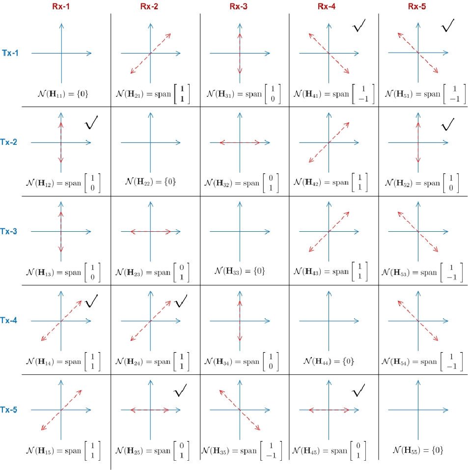
Consider a $2\times 2$ , 5-pair interference network. Each Tx-Rx pair attempts to transmit 1 data stream (i.e. $d^{\max}_{n}=1$ , $\forall n\in\{1,2,3,4,5\}$ ). If the network is fully connected (all channel matrices are rank 2), the freedoms in each precoder $\mathbf{v}_{n}\in\mathbb{C}^{2\times 1}$ and decorrelator $\mathbf{u}_{m}\in\mathbb{C}^{1\times 2}$ is given by $\mbox{dim}(\mathcal{G}(1,2))=1$ , where the Grassmannian [16, 17] $\mathcal{G}(x,y)$ denotes the set of all $x$ -dimensional subspaces in $\mathbb{C}^{y}$ , and the number of constraints induced by each cross link ( $\mathbf{u}_{m}\mathbf{H}_{mn}\mathbf{v}_{n}=0$ , $n\neq m$ ) is 1. If we assign data streams to $k$ Tx-Rx pairs, there are in total $2k$ freedoms in the precoders and the decorrelators and $k(k-1)$ interference alignment constraints. Hence, from the IA feasibility condition [6], we have $k(k-1)\leq 2k\Rightarrow k\leq 3$ . In other words, the achievable DoF is upper bounded by 3.

Now suppose the network is partially connected such that the channel matrices of all cross links are rank 1 with null spaces given by the red arrows in Fig. 3. Then we have IA constraints (10), (11) are satisfied under the following policy: Assign data streams to Tx-Rx pairs 1,2,4,5 ( $\{1,2,...,K\}$ ={1,2,4,5}), with precoders $\mathbf{v}_{1}=\frac{\sqrt{2}}{2}\left[\begin{array}[]{c}1\\ -1\end{array}\right]$ , $\mathbf{v}_{2}=\left[\begin{array}[]{c}1\\ 0\end{array}\right]$ , $\mathbf{v}_{4}=\frac{\sqrt{2}}{2}\left[\begin{array}[]{c}1\\ 1\end{array}\right]$ , $\mathbf{v}_{5}=\left[\begin{array}[]{c}0\\ 1\end{array}\right]$ , and decorrelators $\mathbf{u}_{1}=(\left[\begin{array}[]{r@{\;\;}r}0&-1\\ 1&0\end{array}\right]\mathbf{H}_{15}\mathbf{v}_{5})^{T}$ , $\mathbf{u}_{2}=(\left[\begin{array}[]{r@{\;\;}r}0&-1\\ 1&0\end{array}\right]\mathbf{H}_{21}\mathbf{v}_{1})^{T}$ , $\mathbf{u}_{4}=(\left[\begin{array}[]{r@{\;\;}r}0&-1\\ 1&0\end{array}\right]\mathbf{H}_{42}\mathbf{v}_{2})^{T}$ , $\mathbf{u}_{5}=(\left[\begin{array}[]{r@{\;\;}r}0&-1\\ 1&0\end{array}\right]\mathbf{H}_{54}\mathbf{v}_{4})^{T}$ . Since 4 Tx-Rx pairs can have data streams simultaneously, 1 extra DoF is achieved compared to the fully connected case.

The example above illustrates how partial connectivity can contribute to network performance gains. However, as we shall explain below, there are various technical challenges to exploit the benefit of partial connectivity for general scenarios.

III-A2 The difficulty in exploiting the benefit of partial connection

•

Interference overlapping versus interference nulling: Classical interference alignment schemes [4] reduce interference dimension by “overlapping” the interferences from different Txs. However, when partial connectivity is considered, “overlapping” interferences is no longer the only method to reduce interference dimension. Part of the interference can also be eliminated by utilizing the null spaces of the channel states. For instance, in the previous example, by setting $\mathbf{v}_{1}=\frac{\sqrt{2}}{2}\left[\begin{array}[]{c}1\\ -1\end{array}\right]$ , we eliminate the interference from Tx 1 to Rx 4 and 5 by utilizing the null space of $\mathbf{H}_{41}$ and $\mathbf{H}_{51}$ . In practice, we should dynamically combine these two approaches in order to better exploit the nulling opportunities as well as alignment opportunities in a partially connected interference network. However, a combined design may depend heavily on the specific realization of the connection topology and a combination criteria that can work for general connection topologies is not yet clear.
•

Freedoms versus constraints: Another perspective of the technical challenges is on the feasibility conditions in quasi-static MIMO interference networks. In [6], a symmetrical MIMO interference system is feasible if and only if the number of freedoms in transceiver design is no less than the number of independent constraints induced by interference alignment requirements. In order to reduce the number of the independent constraints in a partially connected network, we need to restrict the precoders and decorrelators to a lower rank subspace. On the other hand, restricting precoders and decorrelators to a lower rank subspace reduces the number of the freedoms in the precoders and decorrelators. The conflict between freedoms in transceiver design and independent constraints makes the subspace selection very challenging.
•

Exponential complexity in checking IA feasibility conditions: As revealed in [6], checking the IA feasibility condition requires comparison of freedoms versus constraints for every possible combination of the interference nulling constraints. This process involves $2^{K(K-1)}-1$ comparisons, where $K$ is the number of Tx-Rx pairs. Such a complexity is intolerable in practice. Hence, a low complexity algorithm for checking the feasibility condition on a real-time basis is needed.

III-B Dynamic Interference Mitigation Scheme for a 5-Pair 2 $\times$ 2 Partially Connected Interference Network

The following observation is the key insight of the proposed algorithm:

Observation: In a partially connected MIMO interference network, by properly restricting precoders $\mathbf{V}_{m}$ and decorrelators $\mathbf{U}_{n}$ to a lower rank subspace, we can eliminate “many” independent constraints at a cost of only a few “free variables” and hence extend the IA feasibility region.

In this section, we shall use the example of a 5-pair 2 $\times$ 2 partially connected interference network described in SectionIII-A1 to illustrate the main ideas of the proposed scheme.

•

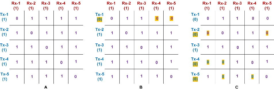
Step 1 Initialization: Note that all the 5 direct links have sufficient rank (rank $(\mathbf{H}_{nn})=2>1$ , $n\in\{1,2...,5\}$ ), initialize $\mathbb{D}=\{1,1,1,1,1\}$ to see if the network is feasible with all Tx-Rx pairs active.

After the initialization, the number of the freedoms in transceiver design and the number of the IA constraints is illustrated in Fig. 4A. The numbers in red and blue denote the freedoms in the corresponding decorrelators and precoders, respectively, and the numbers in purple denote the number of the IA constraints.
•

Step 2 Find out the common subspaces in partial connectivity: As indicated by the“ $\surd$ ” signs in Fig. 3, from Tx 1 to Rx 4 and 5, there is a one dimensional common subspace in partial connectivity state: $\mathcal{N}(\mathbf{H}_{41})=\mathcal{N}(\mathbf{H}_{51})=\mbox{span}\left[\begin{array}[]{c}1\\ -1\end{array}\right]$ . Similarly, from Tx 2 to Rx 1 and 5, from Tx 4 to Rx 1 and 2, from Tx 5 to Rx 2 and 4, there are common null spaces.
•

Step 3 Select subspaces to reduce the number of IA constraints: Set $\mathbf{v}_{1}=\left[\begin{array}[]{c}\frac{\sqrt{2}}{2}\\ -\frac{\sqrt{2}}{2}\end{array}\right]$ , we have $\mathbf{H}_{m1}\mathbf{v}_{1}=\mathbf{0}$ , $m\in\{4,5\}$ . Hence, as indicated by the highlight parts in Fig. 4B, we reduce 2 constraints at a cost of 1 freedom. Similarly, as indicated by the highlight parts in Fig. 4C, since Tx 2,4,5 each has two cross links with overlapping null spaces, we can reduce 2 constraints at a cost of 1 freedom by setting the precoder vectors to be the basis vectors of the corresponding null spaces.
•

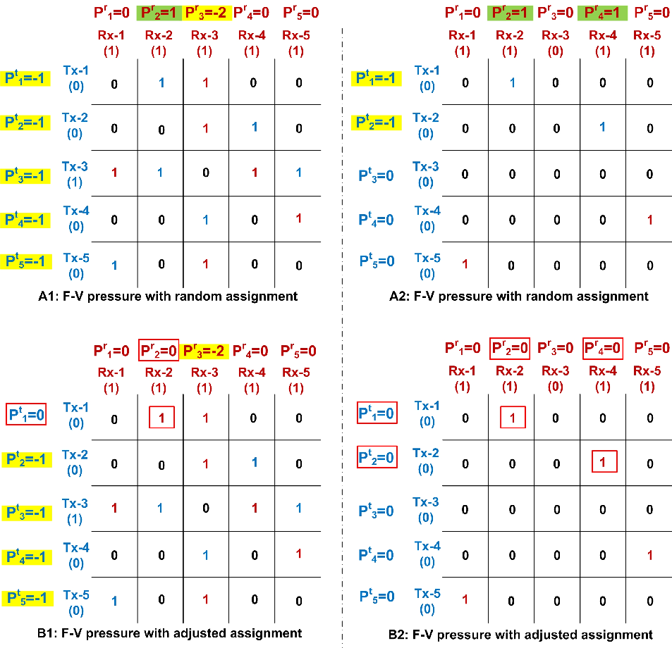
Step 4 Check the feasibility conditions: The number of the remaining freedoms and constraints after step 3 is illustrated in Fig. 4C. Randomly assign the constraints to the corresponding Txs or Rxs (as indicated by the color of the numbers, deep-blue and deep-red indicate the number is assigned to the Tx or the Rx, respectively), we get Fig. 5A1. In this figure, some nodes are “overloaded” in the sense that the number of freedoms at this node minus the number of constraints assigned to this node is negative (highlighted using yellow) while some nodes still have extra freedoms (highlighted using green). Hence, as illustrated in Fig. 5A2, we can reassign the constraints so that we can have less overloaded nodes (the changes are highlighted using red boxes). However, in Fig. 5A2, there are still some overloaded nodes while no nodes have extra freedoms, hence the network is not feasible.
•

Step 5 Turn off the most “constraint demanding” stream: As illustrated in Fig. 5A2, if we remove Tx-Rx pair 1 from the active set $\{1,2,...,K\}$ , we reduce 1 freedom (the freedom in $\mathbf{v}_{1}$ ) and 4 constraints (link Tx 1 to Rx 2,3 and Tx 3,5 to Rx 1). Hence, the freedom-constraint gain by removing Tx-Rx pair 1 is $(-1)-(-4)=3$ . Similarly, the freedom-constraint gains by removing Tx-Rx pair 2,4,5 are also $3$ , whereas the gain by removing Tx-Rx pair 3 is $(-2)-(-8)=6$ . Since $6>3$ , we remove the stream of Tx-Rx pair 3, i.e. let $\mathbb{D}=\{1,1,0,1,1\}$ and return to Step 3.
•

Repeat Step 3 $\sim$ 4: After removing the stream of Tx-Rx pair 3, repeat Step 3 $\sim$ 4 and the number of the remaining freedoms and constraints after subspace selection is illustrated in Fig. 5B1. As revealed by Fig. 5B2, the IA constraints can be assigned properly so that no node is overloaded, the network is feasible. Continue to Step 6.
•

Step 6 Precoder and decorrelator determination: Based on the results given in Steps 1 $\sim$ 5, use the minimum interference leakage iteration [7] to determine the precoders and decorrelators and we get the policy proposed in Section III-A1.

Remark III.1 (Low Complexity IA Feasibility Checking in Step 4)

To avoid the exponential complexity in IA feasibility checking, we have proposed a low complexity method, namely the freedom-constraint assignment with worst case complexity $\mathcal{O}(K^{3})$ only. Furthermore, we shall formally prove in Appendix D that this method is indeed a necessary and sufficient condition of the IA feasibility conditions (14) in the general case. ∎

III-C Dynamic Interference Mitigation Scheme - General Case

Inspired by the example above, we shall propose a two-stage algorithm, namely stream assignment and subspace determination stage and precoder / decorrelator determination stage. The first stage algorithm (which corresponds to Step 1 $\sim$ 5 in the example illustrated above) determines the stream assignment pattern $\mathbb{D}=\{d_{1},d_{2},...,d_{K}\}$ and the subspaces for the precoders $\mathbb{S}^{t}_{n}$ and decorrelators $\mathbb{S}^{r}_{m}$ for $n,m\in\{1,2,...,K\}$ based on the partial connectivity state $\{{\mathcal{N}(\mathbf{H}_{mn})},{\mathcal{N}^{H}(\mathbf{H}_{mn})}\}$ , $m,n\in\{1,2,...,K\}$ . Based on the outputs of the stage I algorithm and the channel state, the stage II algorithm (which corresponds to Step 6 in the example illustrated above) determines the precoders/decorrelators. In the next two subsections, we shall elaborate the details of the stage I and stage II algorithms, respectively.

III-C1 Stage I: Stream Assignment and Subspace Determination

Suppose the row vectors in precoder $\mathbf{V}_{n}$ and the column vectors in decorrelator $\mathbf{U}_{m}$ are constrained to the linear spaces $\mathbb{S}^{t}_{n}\subseteq\mathbb{C}^{N_{t}\times 1}$ and $\mathbb{S}^{r}_{m}\subseteq\mathbb{C}^{1\times N_{r}}$ , respectively. Denote $S^{t}_{n}=|\mathbb{S}^{t}_{n}|$ , $S^{r}_{m}=|\mathbb{S}^{r}_{m}|$ , where $|\mathbb{X}|$ denotes the rank of linear space $\mathbb{X}$ . Then (10) and (11) can be rewritten as:

	$\displaystyle\mbox{rank}(\mathbf{U}_{n}\mathbf{H}_{nn}\mathbf{V}_{n})=\mbox{rank}(\mathbf{U}^{\prime}_{n}\mathbf{S}^{r}_{n}\mathbf{H}_{nn}\mathbf{S}^{t}_{n}\mathbf{V}^{\prime}_{n})$	$\displaystyle=$	$\displaystyle d_{n}$		(12)
	$\displaystyle\mathbf{U}_{m}\mathbf{H}_{mn}\mathbf{V}_{n}=\mathbf{U}^{\prime}_{m}\mathbf{S}^{r}_{m}\mathbf{H}_{mn}\mathbf{S}^{t}_{n}\mathbf{V}^{\prime}_{n}$	$\displaystyle=$	$\displaystyle\mathbf{0}$		(13)

where the column vectors of the $N_{t}\times S^{t}_{n}$ matrix $\mathbf{S}^{t}_{n}$ and the $S^{r}_{m}\times N_{r}$ matrix $\mathbf{S}^{r}_{m}$ span the spaces $\mathbb{S}^{t}_{n}$ and $\mathbb{S}^{r}_{m}$ , respectively. Note that the constrained precoder $\mathbf{V}^{\prime}_{n}$ and the constrained decorrelator $\mathbf{U}^{\prime}_{m}$ are $S^{t}_{n}\times d_{n}$ and $d_{m}\times S^{r}_{m}$ matrices, respectively.

Before we elaborate the details of the stage I processing, we shall first define the notion of a proper MIMO interference system.

Definition III.1 (Proper MIMO Interference Systems for the General Case)

The MIMO interference system is proper for interference alignment if:

	$\displaystyle\sum_{(n,m)\in\mathbb{G}}\min\left(d_{m},\|\mathbb{S}^{r}_{m}\cap(\mathcal{N}^{H}(\mathbf{H}_{mn}))^{\bot}\|\right)\cdot\min\left(\|\mathbb{S}^{t}_{n}\cap\mathcal{N}(\mathbf{H}_{mn})^{\bot}\|,d_{n}\right)$
	$\displaystyle\leq\sum_{n\in\mathbb{G}_{T}}d_{n}(S^{t}_{n}-d_{n})+\sum_{m\in\mathbb{G}_{R}}d_{m}(S^{r}_{m}-d_{m})$		(14)

$\forall\mathbb{G}_{T},\mathbb{G}_{R}\subseteq\{1,2,...,K\}$ , $\mathbb{G}=(\mathbb{G}_{R}\times\mathbb{G}_{T})\backslash\{(n,n)$ $,n\in\mathbb{G}_{R}\cap\mathbb{G}_{T}\}$ , where “ $\times$ ” denotes Cartesian product. ∎

Remark III.2 (Physical Meaning of Definition III.1)

As proved in Appendix B, the left hand side of (14) represents the total number of interference alignment constraints of the links from a Tx in set $\mathbb{G}_{n}$ to a Rx in set $\mathbb{G}_{m}$ , and the first and second term on the right hand side of (14) represent the sum of the free variables in $\mathbf{V}^{\prime}_{n}$ , $n\in\mathbb{G}_{n}$ and $\mathbf{U}^{\prime}_{m}$ , $m\in\mathbb{G}_{m}$ , respectively. Hence, (14) means that for any subset of Tx-Rx combination $\mathbb{G}_{n}\oplus\mathbb{G}_{m}\subseteq\{1,2,...,K\}\oplus\{1,2,...,K\}$ , the number of constraints is no more than the number of free variables. ∎

The main steps of the Stage I processing algorithm for the general $K$ -pair partially connected interference network is illustrated below. Steps 1 $\sim$ 5 below corresponds to the Steps 1 $\sim$ 5 for the 5-Pair example.

Stage 1 (Stream Assignment and Subspace Determination)

•

Step1 Initialization: Initialize the number of stream assigned to each Tx-Rx pair to be the minimum of the rank of the direct link and the number of streams claimed by this Tx-Rx pair, i.e. $d_{n}=\min(\mbox{rank }(\mathbf{H}_{nn}),d^{\max}_{n})$ , $\forall n\in\{1,2,...,K\}$ .
•
Step2 Calculate the common null spaces¹¹ 1 The worst case complexity of this step is $\mathcal{O}(K2^{K^{\prime}-1})$ , where $K^{\prime}=\max_{n}(\max(|\mathbb{K}^{t}_{n}|,|\mathbb{K}^{r}_{n}|))$ . In practice, due to path loss, $K^{\prime}$ usually does not scale with $K$ . Hence, the $2^{K^{\prime}-1}$ term is only a moderate constant which does not scale with the size of the network in most of the interesting scenarios. : For every Tx-n, $n\in\{1,2,...,K\}$ , calculate the common subspaces of the null spaces of the cross links from this Tx within the effective subspace of the direct link , i.e. $\mathcal{N}(\{\mathbf{H}_{mn}:m\in\mathbb{K}_{sub}\})=\left(\cap_{m\in\mathbb{K}_{sub}}\mathcal{N}(\mathbf{H}_{mn})\right)\cap(\mathcal{N}(\mathbf{H}_{nn}))^{\perp}$ , $\mathbb{K}_{sub}\subseteq\{1,2,...,K\}$ as follows:
- –
  
  Denote $\mathbb{K}^{t}_{n}=\{m:m\in\{1,2,...,K\},\mathcal{N}(\mathbf{H}_{mn})\neq\mathbb{C}^{N_{t}\times 1}(\mbox{i.e. }\mathbf{H}_{nm}\neq\mathbf{0})\}$ , Initialize $\mathcal{N}(\emptyset)=(\mathcal{N}(\mathbf{H}_{nn}))^{\perp}$ , $\mathcal{N}(\{\mathbf{H}_{mn}\})=\mathcal{N}(\mathbf{H}_{mn})\cap(\mathcal{N}(\mathbf{H}_{nn}))^{\perp}$ , $\forall m\in\mathbb{K}^{t}_{n}$ , and subset cardinality parameter $C=2$ .
- –
  
  For every $\mathbb{K}_{sub}\subseteq\mathbb{K}^{t}_{n}$ with $|\mathbb{K}_{sub}|=C$ , if all the subsets of $\mathbb{K}_{sub}$ with cardinality $(C-1)$ are not $\{0\}$ , calculate $\mathcal{N}(\{\mathbf{H}_{mn}:m\in\mathbb{K}_{sub}\})=\mathcal{N}(\{\mathbf{H}_{mn}:m\in\mathbb{K}_{sub}\backslash\{m^{\prime}\}\}\cap\mathcal{N}(\mathbf{H}_{m^{\prime}n})$ , where $m^{\prime}$ is an arbitrary element in $\mathbb{K}_{sub}$ . Update $C=C+1$ . Repeat this process until $\mathcal{N}(\{\mathbf{H}_{mn}:m\in\mathbb{K}_{sub}\})=\{0\}$ , $\forall\mathbb{K}_{sub}\subseteq\mathbb{K}^{t}_{n}$ with $|\mathbb{K}_{sub}|=C$ or $C=|\mathbb{K}^{t}_{n}|$ .
- –
  
  For every $\mathbb{K}_{sub}\subseteq\mathbb{K}^{t}_{n}$ with $\mathcal{N}(\{\mathbf{H}_{mn}:m\in\mathbb{K}_{sub}\})\neq\{0\}$ , set $\mathcal{N}(\{\mathbf{H}_{mn}:m\in\mathbb{K}_{sub}\cup(\{1,2,...,K\}\backslash\mathbb{K}^{t}_{n})\})=\mathcal{N}(\{\mathbf{H}_{mn}:m\in\mathbb{K}_{sub}\})$ .
For every Rx-m, $m\in\{1,2,...,K\}$ , calculate $\mathcal{N}^{H}(\{\mathbf{H}_{mn}:n\in\mathbb{K}_{sub}\})=(\cap_{n\in\mathbb{K}_{sub}}\mathcal{N}^{H}(\mathbf{H}_{mn}))\cap(\mathcal{N}^{H}(\mathbf{H}_{mm}))^{\perp}$ , $\mathbb{K}_{sub}\subseteq\{1,2,...,K\}$ using a similar process.

•

Step3 Design Subspace constraints $\mathbb{S}^{t}_{n}$ and $\mathbb{S}^{r}_{m}$ : For every Tx $n$ , $n\in\{1,2,...,K\}$ , generate a series of potential subspace constraints $\mathbb{S}^{t}_{n}(d),d\in\{d_{n},d_{n}+1,...,N_{t}\}$ with $|\mathbb{S}^{t}_{n}(d)|=d$ , based on the principe that a subspace which has higher null space ‘‘weight”²² 2 The weight of $\mathcal{N}(\{\mathbf{H}_{mn}:m\in\mathbb{K}_{sub}\})$ is $\sum_{m\in\mathbb{K}_{sub}}d_{m}$ . From the left hand side of (14), this weight is the maximum number of IA constraints that one can mitigate by selecting a one dimensional subspace in $\mathcal{N}(\{\mathbf{H}_{mn}:m\in\mathbb{K}_{sub}\})$ . is selected with higher priority. Choose the subspace constraint $\mathbb{S}^{t}_{n}$ from the potential subspace constraints: $\mathbb{S}^{t}_{n}=\mathbb{S}^{t}_{n}(d^{*})$ , where:

	$\displaystyle d^{*}$	$\displaystyle=$	$\displaystyle\arg\max_{d\in\{d_{n},d_{n}+1,...,N_{t}-\|\mathcal{N}(\mathbf{H}_{nn})\|\}}d_{n}(d-d_{n})-$		(15)
			$\displaystyle\sum_{m\neq n}^{\{1,2,...,K\}}\min(d_{m},\|({\mathcal{N}^{H}(\mathbf{H}_{mn})})^{\bot}\|)\min(\|\mathbb{S}^{t}_{n}(d)\cap\mathcal{N}(\mathbf{H}_{mn})^{\bot}\|,d_{n}).$		(15)

For every Rx $m$ , $m\in\{1,2,...,K\}$ , use a similar process to generate $\mathbb{S}^{r}_{m}(d)$ , $d\in\{d_{m},d_{m}+1,...,N_{r}\}$ and set $\mathbb{S}^{r}_{m}=\mathbb{S}^{r}_{m}(d^{*})$ , where

	$\displaystyle d^{*}$	$\displaystyle=$	$\displaystyle\arg\max_{d\in\{d_{m},d_{m}+1,...,N_{r}-\|\mathcal{N}^{H}(\mathbf{H}_{mm})\|\}}d_{m}(d-d_{m})-$		(16)
			$\displaystyle\sum_{n\neq m}^{\{1,2,...,K\}}\mbox{min}(d_{m},\|\mathbb{S}^{r}_{m}(d)\cap(\mathcal{N}^{H}(\mathbf{H}_{mn}))^{\bot}\|)\min(\|\mathbb{S}^{t}_{n}\cap({\mathcal{N}(\mathbf{H}_{mn})})^{\bot}\|,d_{n}).$		(16)

•

Step4 Low complexity feasibility checking: Denote $v^{t}_{n},v^{r}_{m}$ , $n,m\in\{1,2,...,K\}$ as the number of the freedoms at Tx $n$ and Rx $m$ , respectively. Set $v^{t}_{n}=d_{n}(|\mathbb{S}^{t}_{n}|-d_{n})$ , $v^{r}_{m}=d_{m}(|\mathbb{S}^{r}_{m}|-d_{m})$ . Denote $c_{mn}$ , $n\neq m\in\{1,2,...,K\}$ as the number of constraints required to eliminate the interference from the Tx $n$ to the Rx $m$ . Set $c_{mn}=\min\left(d_{m},|\mathbb{S}^{r}_{m}\cap({\mathcal{N}^{H}(\mathbf{H}_{mn})})^{\bot}|\right)$ $\min\left(d_{n},|\mathbb{S}^{t}_{n}\cap{\mathcal{N}(\mathbf{H}_{mn})}^{\bot}|\right)$ and $c_{mm}=0$ , $\forall n\neq m\in\{1,2,...,K\}$ . Use freedom-constraint assignment to check if the system is proper (Please refer to Appendix C for details.) If the network is not proper, go to Step 5. Otherwise, let $\mathbb{D}^{*}=\{d^{*}_{1},d^{*}_{2},...,d^{*}_{K}\}=\mathbb{D}$ , $\mathbb{S}^{t*}_{n}=\mathbb{S}^{t}_{n}$ , $\mathbb{S}^{r*}_{m}=\mathbb{S}^{r}_{m}$ , $\forall n,m\in\{1,2,...,K\}$ , and exit the algorithm.

•

Step5 : Update $\mathbb{D}=\{d_{1},d_{2},...d_{\tilde{n}}-1,...,d_{K}\}$ and go back to Step 3, where $\tilde{n}$ is given by

\displaystyle\tilde{n}=\arg\max_{n\in\{1,2,...,K\}}\left(\sum_{m=1}^{K}(c_{mn}+c_{nm}-c^{\prime}_{mn}-c^{\prime}_{nm})-(v^{t}_{n}+v^{r}_{n}-{v^{t}_{n}}^{\prime}-{v^{r}_{n}}^{\prime})\right)

(17)

where $\{{v^{t}_{n}}^{\prime},{v^{r}_{n}}^{\prime}\}$ and $\{c^{\prime}_{mn},c^{\prime}_{nm}\}$ , $m\in\{1,2,...,K\}$ are the number of freedoms and IA constraints under updated subspace constraints ${\mathbb{S}^{t}_{n}}^{\prime}$ and ${\mathbb{S}^{r}_{n}}^{\prime}$ given by (15) and (16) with $d^{\prime}_{n}=d_{n}-1$ , respectively.

Remark III.3 (stream assignment and subspace design criterion in Stage I Algorithm)

As revealed in [6], the IA feasibility condition is the major limitation of the DoF performance achieved by MIMO interference networks. Hence, in order to enhance the network DoF performance, subspace constraints $\{\mathbb{S}^{t*}_{n},\mathbb{S}^{r*}_{m}\}$ and stream assignment $\mathbb{D}^{*}_{n}$ are designed to alleviate the IA feasibility condition as much as possible.

•

Recall (44), (46), we can see that (15), (16) choose the dimension of subspace constraints $d^{*}$ to maximize the difference between the number of freedoms in precoder (or decorrelator) design minus the number of IA constraints endued by the Tx (or Rx).
•

The right hand side of (17) represents the number of IA constraint - freedom in transceiver design saved by removing one stream from Tx-Rx pair $n$ . The higher this number, the more “constraint demanding” this stream is. Hence, it should be removed first so that the network can become IA feasible easier. ∎

Lemma 1 (Property of the low complexity IA feasibility checking)

A partially connected MIMO interference network with stream assignment $\mathbb{D}$ and potential signal subspace $\{\mathbb{S}^{t}_{n},\mathbb{S}^{r}_{m}\}$ policy is proper (i.e. satisfies (14)) if and only if it can pass the low complexity IA feasibility checking in Appendix C. Moreover, the worst case complexity of the proposed checking scheme is $\mathcal{O}(K^{3})$ .

Proof:

Please refer to Appendix D for the proof. ∎From Lemma 1, and Definition III.1, we have the following theorem:

Theorem III.1 (Property of $\{\mathbb{S}^{t}_{n},\mathbb{S}^{r}_{m}\}$ and $\mathbb{D}^{*}$ )

Under Assumption II.1, the potential signal subspace $\{\mathbb{S}^{t*}_{n},\mathbb{S}^{r*}_{m}\}$ , together with the stream assignment pattern $\mathbb{D}^{*}$ from Stage 1 form a proper system.

III-C2 Stage II: Precoder and Decorrelator Determination

In this section, we shall elaborate the stage II processing, which determines the precoders $\{\mathbf{V}_{n}\}$ and the decorrelators $\{\mathbf{U}_{m}\}$ under the subspace constraints determined in stage I. Specifically, since the subspace constraint can be represented by the constrained precoder and decorrelator as in (12), (13), the precoder and decorrelator design is given by the following optimization objective which minimizes the total interference leakage power in the network:

$\min_{\mathbf{U}^{\prime}_{m},\mathbf{V}^{\prime}_{n}}\sum_{n=1,d^{*}_{n}>0}^{K}\sum_{m=1,\neq n\atop d^{*}_{m}>0}^{K}\frac{P_{n}}{d^{*}_{n}}\mbox{trace}\left((\mathbf{U}^{\prime}_{m}\mathbf{S}^{r*}_{m}\mathbf{H}_{mn}\mathbf{S}^{t*}_{n}\mathbf{V}^{\prime}_{n})^{H}(\mathbf{U}^{\prime}_{m}\mathbf{S}^{r*}_{m}\mathbf{H}_{mn}\mathbf{S}^{t*}_{n}\mathbf{V}^{\prime}_{n})\right)$ .

The following algorithm is guaranteed to converge to a local optimum [7].

Stage 2 (Precoder and Decorrelator Determination)

Given $\{\mathbb{D}^{*},\mathbb{S}^{t*}_{n},\mathbb{S}^{r*}_{m}\}$ , determined by Stage I:

•

Step1 Initialization : Denote $\mathbf{S}^{r}_{m}$ and $\mathbf{S}^{t}_{n}$ as the structure matrices for decorrelators and precoders: $\mathbf{U}_{m}=\mathbf{U}^{\prime}_{m}\mathbf{S}^{r}_{m}$ , $\mathbf{V}_{n}=\mathbf{S}^{t}_{n}\mathbf{V}^{\prime}_{n}$ . Set $\mathbf{S}^{t*}_{n}$ and $\mathbf{S}^{r*}_{m}$ to be the aggregation of the basis vectors in $\mathbb{S}^{t}_{n}$ and $\mathbb{S}^{r}_{m}$ , respectively. Randomly generate $\mathbf{V}^{\prime}_{n}$ .
•

Step2 Minimize interference leakage at the receiver side: At each Rx $m$ , such that $d^{*}_{m}>0$ , update $\mathbf{U}^{\prime}_{m}$ : $\mathbf{u}^{\prime}_{m}(d)=\left(\nu_{d}\left[\sum_{n=1,\neq m\atop d^{*}_{n}>0}^{K}\frac{P_{n}}{d^{*}_{n}}(\mathbf{S}^{r*}_{m}\mathbf{H}_{mn}\mathbf{S}^{t*}_{n}\mathbf{V}^{\prime}_{n})(\mathbf{S}^{r*}_{m}\mathbf{H}_{mn}\mathbf{S}^{t*}_{n}\mathbf{V}^{\prime}_{n})^{H}\right]\right)^{H}$ , where $\mathbf{u}^{\prime}_{m}(d)$ is the $d$ -th row of $\mathbf{U}^{\prime}_{m}$ , $\nu_{d}[\mathbf{A}]$ is the eigenvector corresponding to the d-th smallest eigenvalue of $\mathbf{A}$ , $d\in\{1,2,...,{d^{*}_{m}}\}$ .
•

Step3 Minimize interference leakage at the transmitter side: At each Tx $n$ such that $d^{*}_{n}>0$ , update $\mathbf{V}^{\prime}_{n}$ : $\mathbf{v}^{\prime}_{n}(d)=\nu_{d}\left[\sum_{m=1,\neq n\atop d^{*}_{m}>0}^{K}\frac{P_{n}}{d^{*}_{n}}(\mathbf{U}^{\prime}_{m}\mathbf{S}^{r*}_{m}\mathbf{H}_{mn}\mathbf{S}^{t*}_{n})^{H}(\mathbf{U}^{\prime}_{m}\mathbf{S}^{r*}_{m}\mathbf{H}_{mn}\mathbf{S}^{t*}_{n})\right]$ , where $\mathbf{v}^{\prime}_{m}(d)$ is the $d$ -th column of $\mathbf{V}^{\prime}_{m}$ , $d\in\{1,2,...,{d^{*}_{n}}\}$ .
Repeat Step 2 and 3 until $\mathbf{V}^{\prime}_{n}$ and $\mathbf{U}^{\prime}_{m}$ converges. Set $\mathbf{V}^{*}_{n}=\mathbf{S}^{t}_{n}\mathbf{V}^{\prime}_{n}$ and $\mathbf{U}^{*}_{m}=\mathbf{U}^{\prime}_{m}\mathbf{S}^{r}_{m}$ , $\forall n,m\in\{1,2,...,K\}$ .

Remark III.4 (Backward Compatibility of the Proposed Scheme)

When the system is fully connected (i.e. $\mathcal{N}(\mathbf{H}_{mn})=\mathcal{N}^{H}(\mathbf{H}_{mn})=\{0\}$ , $\forall n,m\in\{1,2,...,K\}$ ), it is easy to check in Algorithm 1, $\mathbb{S}^{t*}_{n}=\mathbb{C}^{N_{t}\times 1}$ and $\mathbb{S}^{r*}_{m}=\mathbb{C}^{1\times N_{r}}$ ; this means that in fully connected quasi-static MIMO interference networks, the proposed scheme reduces to the conventional IA schemes proposed in [6] and [7]. When $N_{t}>N_{r}$ , the algorithm shall first utilize the null spaces on the Tx side and design $\mathbb{S}^{t*}_{n}$ to null off part of the interference, which is similar to [3]. However, given a general partial connectivity topology $\{\mathcal{N}(\mathbf{H}_{mn}),\mathcal{N}^{H}(\mathbf{H}_{mn})\}$ , the algorithm generalizes the conventional interference alignment by dynamically combining the interference alignment and interference nulling approaches. ∎

IV Performance Analysis

In this section, we shall derive the analytical DoF performance achieved by the proposed scheme in a symmetrical partially connected MIMO interference network. In fact, although the algorithm itself applies to general typologies, analyzing such cases can be prohibitively complicated. Since there are too many parameters in the general partial connectivity parameters $\{\mathcal{N}(\mathbf{H}_{mn}),\mathcal{N}^{H}(\mathbf{H}_{mn})\}$ , $m,n\in\{1,2,...,K\}$ in Section II-A, we shall focus on a symmetrical $K$ -pair partially connected MIMO interference network in which the partial connectivity is induced by both the path loss and the local scattering.

Definition IV.1 (Symmetrical Partially Connected MIMO Interference Channels)

Consider a $K$ -pair partially connected MIMO interference network with the following configuration. Each Tx has $N_{t}$ antennas and each Rx has $N_{r}$ antennas. Each Tx-Rx claims $d^{\max}_{n}=d_{f}$ data streams, $\forall n\in\{1,2,...,K\}$ . The partial connectivity states (elaborated below) are expressed in terms of three key parameters $L$ , $E_{1}$ and $E_{2}$ , which characterize the connection density, the rank of the direct links and the rank of the cross links, respectively. Please refer to Appendix E for the details.

	$\displaystyle\mathcal{N}(\mathbf{H}_{mn})=\left\{\begin{array}[]{l}\left(\mbox{span}(\mathbf{e}_{N_{t}}(q))\right)^{\perp},q\in\mathbb{E}_{1}\mbox{ if: }m=n\\ \left(\mbox{span}(\mathbf{e}_{N_{t}}(q))\right)^{\perp},q\in\mathbb{E}_{2}(n-m)\mbox{ if: }{0<\|n-m\|\leq L\mbox{ or }\|n-m\|\geq K-L}\\ \mathbb{C}^{N_{t}\times 1}\mbox{ otherwise}\end{array}\right.$
	$\displaystyle\mathcal{N}^{H}(\mathbf{H}_{mn})=\left\{\begin{array}[]{l}\left(\mbox{span}((\mathbf{A}_{R}\mathbf{h}^{ang}_{mn}(q))^{H})\right)^{\perp},q\in\mathbb{E}_{1}\mbox{ if: }m=n\\ \left(\mbox{span}((\mathbf{A}_{R}\mathbf{h}^{ang}_{mn}(q))^{H})\right)^{\perp},q\in\mathbb{E}_{2}(n-m)\mbox{ if: }\begin{array}[]{l}{0<\|n-m\|\leq L\mbox{ or }\|n-m\|}\\ {\geq K-L}\end{array}\\ \mathbb{C}^{1\times N_{r}}\mbox{ otherwise}\end{array}\right.$

where $\mathbf{H}^{ang}_{mn}$ , $\mathbf{A}_{R}$ and $\mathbf{e}_{N_{t}}(q)$ are defined in (2), (4) and (5), respectively. $\mathbf{h}^{ang}_{mn}(s)\in\mathbb{C}^{N_{r}\times 1}$ is the $s$ -th column of $\mathbf{H}^{ang}_{mn}$ . $\mathbb{E}_{1}$ and $\mathbb{E}_{2}(n-m)$ are subsets of $\{1,2,...,N_{t}\}$ , with $|\mathbb{E}_{1}|=E_{1}$ , $|\mathbb{E}_{2}(n-m)|=E_{2}$ , $\forall n,m$ . ∎

Theorem IV.1 (Performance of the Partially Connected $K$ -pair MIMO Systems)

The proposed algorithm could achieve $\mathbb{D}^{*}=\{d_{f},d_{f},...,d_{f}\}$ if

\displaystyle d_{f}\leq\max\left(\frac{E_{1}+\min(E_{1},N_{r})}{\min(K-1,2L)+2},\frac{\min(E_{1},N_{r})}{\min(K-1,2L)\frac{E_{2}}{N_{t}}+1}\right).

(28)

Proof:

Please refer to Appendix F for the proof. ∎

Remark IV.1 (Interpretation of the Results)

Note that the total DoF of the system is given by $Kd_{f}$ , using (28), the system can achieve a total DoF up to:

\displaystyle K{\left\lfloor\max\left(\frac{E_{1}+\min(E_{1},N_{r})}{\min(K-1,2L)+2},\frac{\min(E_{1},N_{r})}{\min(K-1,2L)\frac{E_{2}}{N_{t}}+1}\right)\right\rfloor}

(29)

where the first term and second term in the “max” operation are contributed by restricting the precoders and decorrelators in the subspaces $\mathbb{S}^{t*}_{n}$ and $\mathbb{S}^{r*}_{n}$ obtained in the stage I algorithm. In the following, we shall elaborate various insights regarding how the partial connectivity affects the gain of the system.

•

The gain due to partial connection: In a $K$ -pair fully connected quasi-static MIMO interference channel, the system sum DoF is upper bounded by $\frac{K(N_{t}+N_{r})}{K+1}$ . The partial connectivity improves this bound in two aspects: 1) Gain due to path loss: As path loss limits the maximum number of Rxs that each Tx may interfere, the total DoF of the system can grow on $\mathcal{O}(K)$ ; 2) Gain due to spatial correlation: When the spatial correlation in the cross link is strong (i.e. small $E_{2}$ ), a $\frac{N_{t}}{E_{2}}$ factor gain can be further observed.
•

Connection density versus system performance: For large $K$ , the DoF of the system (29) scales with $\sim\mathcal{O}(\frac{1}{L})$ , which shows that the network density is always a first order constraint on the system DoF.
•

Rank of the cross links versus system performance: The system sum DoF (29) is a (non-strictly) decreasing function of $E_{2}$ , which means system sum DoF grows when the rank of the cross links decrease. When $E_{2}=0$ , the achievable DoF in (29) is reduced to: $K\min(E_{1},N_{r})=K\mbox{rank}(\mathbf{H}_{nn})$ , which means that all Tx-Rx pairs are using all the dimensions of the direct link for transmission.
•

Rank of the direct links versus system performance: The system sum DoF (29) is a (non-strictly) increasing function of $E_{1}$ , which means that the system sum DoF increases when the rank of the direct links increase. High rank direct links help to increase system performance from two aspects: 1) They increase the DoF upper bound that Tx-Rx pairs may achieve. 2) They increase the maximum number of free variables in the precoders and the decorrelators.
•

Backward compatibility with previous results: When the network is fully connected, i.e. $E_{1}=E_{2}=N_{t}$ and $L\geq[\frac{K}{2}]$ , the inequality in (28) is reduced to: $d_{f}\leq\frac{N_{t}+N_{r}}{K+1}$ , which is consistent with the results in [6]. ∎

V Simulation Results

In this section, we shall illustrate the performance of the proposed scheme by simulation. To better illustrate how physical parameters such as the path loss and the scattering environment affect system performance, we consider the following simulation setup based on a randomized MIMO interference channel.

Definition V.1 (Randomized Partially Connected MIMO Interference Channels)

We have 32 Tx-Rx pairs distributed uniformly in a $10km\times 10km$ square as illustrated in Fig. 7. Each node has 12 antennas.³³ 3 We choose relatively large number of Tx-Rx pairs and antennas so that we can have a smooth system performance variation w.r.t. to partial connectivity parameters of the network such as $L$ and $S$ . Each Tx-Rx pair is trying to deliver 2 data streams. Each Tx is transmitting with power $P$ . Denote $D_{mn}$ as the distance between the Tx $n$ and Rx $m$ . The partial connectivity is contributed the following factors:

•

Path loss effect: If $D_{mn}>L$ , we assume the channel from the Tx $n$ to the Rx $m$ is not connected ( $\mathbf{H}_{mn}=\mathbf{0}$ ).
•

Local scattering effect: If $D_{mn}\leq L$ , then due to local scattering, the angular domain channel states $\mathbf{H}^{ang}_{mn}=\{h_{mn}(p,q)\},p,q\in\{1,2,...,12\}$ , has the following property: $h_{mn}(p,q)=0$ if $q$ satisfies (6), where $S$ is the radius of the local scattering otherwise $h_{mn}(p,q)\sim\mathcal{CN}(0,1)$ .

As a result, the partial connectivity parameters for the randomized model is given by

	$\displaystyle\mathcal{N}(\mathbf{H}_{mn})$	$\displaystyle=$	$\displaystyle\left\{\begin{array}[]{l}\mbox{span}(\mathbf{e}_{N_{t}}(q)),q\in\mathbb{Q}_{mn}\mbox{ if: }D_{mn}\leq L\\ \mathbb{C}^{12\times 1}\mbox{ otherwise.}\end{array}\right.$
	$\displaystyle\mathcal{N}^{H}(\mathbf{H}_{mn})$	$\displaystyle=$	$\displaystyle\left\{\begin{array}[]{l}\left(\mbox{span}((\mathbf{A}_{R}\mathbf{h}^{ang}_{mn}(q))^{H})\right)^{\perp},q\not\in\mathbb{Q}_{mn}\mbox{ if: }D_{mn}\leq L\\ \mathbb{C}^{1\times 12}\mbox{ otherwise.}\end{array}\right.$

where $\mathbf{H}^{ang}_{mn}$ , $\mathbf{A}_{R}$ and $\mathbf{e}_{N_{t}}(q)$ are defined in (2), (4) and (5), respectively. $\mathbf{h}^{ang}_{mn}(s)\in\mathbb{C}^{N_{r}\times 1}$ is the $s$ -th column of $\mathbf{H}^{ang}_{mn}$ , and $\mathbb{Q}_{mn}$ is the set of all the column indices $q\in\{1,2,...,12\}$ that satisfies (6). Note that $\mathbb{Q}_{mn}$ is a random set with randomness induced by the random positions of the Tx $n$ and Rx $m$ . ∎

Remark V.1 (Physical Meaning of the Parameters in Definition V.1)

There are two parameters in Definition V.1, $L$ and $S$ . As as illustrated in Fig. 7, $L$ is the maximum distance that a Tx can interfere (e.g. the big circle centered at Tx 1 in the figure) and hence reflects the connection density of the network. $S$ is the radius of the local scattering, from (6), if the direction of a beam from the Tx does not overlap with the local scattering area of a Rx, it cannot be received by the Rx. (e.g. The local scattering area for Rx 1 is the small circles centered at Rx 1. Beam 7, 8 cannot be received by Rx 1 as their direction does not overlap with this circle.) Hence, $S$ controls the rank (spatial correlation level) of the non-zero channels matrices. Larger $S$ corresponds to higher rank channel matrices. ∎

The proposed interference mitigation scheme is compared with 5 reference baselines below:

•

Conventional interference alignment (Baseline 1): The system directly adapts the precoder-decorrelator iteration proposed in [7].
•

Maximum rank signal subspace (Baseline 2): Each node selects a maximum rank subspace constraint, i.e. set $d^{*}$ to be $N_{t}-|\mathcal{N}(\mathbf{H}_{nn})|$ and $N_{r}-|\mathcal{N}^{H}(\mathbf{H}_{mm})|$ in (15) and (16), respectively in Stage I, then uses Stage II to determine the precoders and decorrelators.
•

Minimum rank signal subspace (Baseline 3): Each node selects a minimum rank subspace constraint, i.e. set $d^{*}$ to be $d_{n}$ and $d_{m}$ in (15) and (16), respectively in Stage I, in the stage I algorithm, then use the stage II algorithm to determine the precoders and decorrelators.
•

TDMA (Baseline 4) refers to the case where the Tx-Rx pairs use time division multiple access to avoid all interference.
•

Isotropic transmission (Baseline 5) refers to the case where the Tx and Rx sends and receives the data streams with random precoders and decorrelators without regard of the channel information.

V-A Performance w.r.t. SNR

Fig. 8 illustrates the throughput per Tx-Rx pair versus SNR ( $10\log_{10}(P)$ ). Here $L=5km$ and $S=3km$ . Conventional interference alignment (BL 1) saturates in the high SNR region as traditional IA is infeasible in this dense network. Both the proposed scheme and the Maximum/Minimum signal subspace methods (BL 2 and 3) can achieve throughputs that grow linearly with SNR since the on/off selection in the stage I algorithm guarantees that the system is feasible for IA. However, the proposed scheme achieves much higher DoF ( $\approx 57$ ) than BL 2 ( $\approx 44$ ) and 3 ( $\approx 46$ ), illustrating the importance of carefully designing the signal subspaces. Comparison of the proposed scheme and BL 1 shows that introducing subspace constraints can indeed enlarge the IA feasible region and enhance the system performance in both DoF and throughput sense. Moreover, note that for a $12\times 12$ , $2$ stream per Tx-Rx pair and fully connected interference network, at most total network $22$ DoF can be achieved, the performance of the proposed scheme (50 DoF) show that partial connectivity can indeed be exploit to significantly increase network total DoF.

V-B Performance w.r.t. Partial Connectivity Factors

To better illustrate how different partial connectivity factors such as path loss and spatial correlation affect system performance, we illustrate the sum throughput versus $L$ (the maximum distance that a Tx can interfere a Rx) and $S$ (the radius of the local scattering) under a fixed SNR (40dB) in Fig. 9 and Fig. 10, respectively. By comparing the performance of the proposed scheme with different partial connectivity parameters, we have that the performance of the proposed scheme scales $\mathcal{O}\left(\frac{1}{LS}\right)$ , which illustrates a consistent observation as in Remark IV.1 that weaker partial connectivity can indeed contribute to higher system performance. Moreover, comparison of the proposed algorithm with Baseline 2 and 3 illustrates how we should select signal subspaces $\mathbb{S}^{t*}_{n}$ and $\mathbb{S}^{r*}_{m}$ under different partial connectivity regions. For example, low rank subspace is more effective at high spatial correlation (small $S$ ) while high rank subspace is more effective at low spatial correlation (large $S$ ). Low rank subspace is also more effective compare to high rank subspace in dense networks (large $L$ ) and vice versa. By dynamically selecting signal subspace according to the partial connectivity state of the network, the proposed scheme obtains significant performance gain over a wide range of partial connectivity levels.

VI Conclusion

In this paper, we have investigated how the partial connection can be utilized to benefit the system performance in MIMO interference networks. We considers a general partial connection model which embraces various practical situations such as path loss effects and spatial correlations. We proposed a novel two-stage interference mitigation scheme. The stage I algorithm determines the stream assignment and the subspace constraints for the precoders and decorrelators based on the partial connectivity state. The stage II algorithm determines the precoders and decorrelators based on the stream assignment and the subspace constraints as well as the local channel state information. The signal spaces is designed to mitigate “many” IA constraints at a cost of only a “few” free-variables in precoders and decorrelator so as to extend the feasibility region of the IA scheme. Analysis shows the proposed algorithm can significantly increase system DoF in symmetric partially connected MIMO interference networks. We also compare the performance of the proposed scheme with various baselines and show via simulations that the proposed algorithms could achieve significant gain in system performance of randomly connected interference networks.

Appendix A Physical Interpretation for Virtual Angle Model in MIMO Channel

As has been observed in many previous works [14],[15] the statistical property of the channel states in a MIMO system is strongly affected by the physical propagation environment. For instance, in cellular MIMO systems, the Txs are positioned at high elevations above the scatterers while the Rxs are positioned at low altitude with rich scattering (Fig. 1A). Hence, only the scattering objects surrounding a Rx could effectively reflect signals from the Tx to the Rx as illustrated in Fig. 1B. Following an approach similar to [12, 13], we assume the double directional channel response from the $n$ -th Tx to the $m$ -th Rx ( $n,m\in\{1,2,...,K\}$ ): $\mathbf{H}_{mn}^{a}=\{h_{mn}^{a}(\theta_{t},\theta_{r}),\;\theta_{t},\theta_{r}\in[-{\pi,\pi})\}$ has the following property:

	$\displaystyle h_{mn}^{a}(\theta_{t},\theta_{r})$	$\displaystyle=$	$\displaystyle 0\mbox{ if }\|\theta_{t}\|>\frac{\alpha}{2};$		(36)
	$\displaystyle\mbox{where }\alpha$	$\displaystyle=$	$\displaystyle\left\{\begin{array}[]{l}2\arcsin(\frac{S}{d_{mn}})\;\;\mbox{when: }S\leq{d_{mn}}\\ 2\pi\;\;\;\mbox{else.}\end{array}\right.$

where $d_{mn}$ is the distance between Tx $n$ and to Rx $m$ , $S$ is the local effective scattering radius. Assume the Tx are equipped with uniform linear antenna array (ULA). Hence the virtual angular channel representation [11] is given by:

\displaystyle h^{v}_{mn}(p,q)=\int_{-\pi}^{\pi}\int_{-\pi}^{\pi}h_{mn}(\theta_{t},\theta_{r})f_{N_{r}}\left(\frac{\sin(\theta_{r}-\varphi_{mn})r}{\lambda}-\frac{p}{N_{r}}\right)f_{N_{t}}\left(\frac{\sin(\theta_{t}-\theta_{mn})r}{\lambda}-\frac{q}{N_{t}}\right)d\theta_{r}d\theta_{t}

(40)

where $r$ is the antenna separation, $\lambda$ is the wavelength, $\theta_{mn}$ is the angle between the transmit array normal direction and the direction from Tx $n$ to Rx $m$ , $\varphi_{mn}$ is the angle between receive array normal direction and the direction from Tx $n$ to Rx $m$ , assume the antenna array is critically spaced, i.e. $\frac{r}{\lambda}=\frac{1}{2}$ . $f_{N}(\omega)={\mathbf{e}^{H}_{N}(0)}\mathbf{e}_{N}(\omega)=\frac{1}{N}e^{-j\pi\omega(N-1)}\frac{\sin(\pi N\omega)}{\sin(\pi\omega)}$ .

As illustrated in Fig. 2A, $f_{N}(\omega)$ represents the radiation pattern of ULA [18]. Note that the main-lobes dominate in the radiation pattern (e.g. when $N=8$ , the power of the main-lobes occupy $91\%$ of that in the whole radiation pattern). Hence, as illustrated in Fig. 2B, for simplicity, we use the main-lobe to approximate the radiation pattern, i.e. we use

\displaystyle f^{\prime}_{N}(\omega)=\left\{\begin{array}[]{l}f_{N}(\omega),\mbox{ if: }\omega-\lfloor\omega\rfloor\leq\frac{1}{N}\mbox{ or }\geq\frac{N-1}{N}\\ 0,\mbox{ otherwise.}\end{array}\right.

to replace $f_{N}(\omega)$ in (40). Hence, combining (36), (A) and (40), we have (6).

Appendix B The Number of Freedoms and IA Constraints in Equations (12) and (13)

The freedoms in $\mathbf{V}^{\prime}_{n}$ and $\mathbf{U}^{\prime}_{m}$ of (12) and (13) are given by:

\displaystyle\mbox{dim}(\mathcal{G}(d_{n},S^{t}_{n}))=d_{n}(S^{t}_{n}-d_{f}),\mbox{ and }\mbox{dim}(\mathcal{G}(d_{m},S^{r}_{m}))=d_{m}(S^{r}_{m}-d_{m}),\mbox{ respectively.}

(44)

where the Grassmannian $\mathcal{G}(x,y)$ [16, 17] denotes the set of all $x$ -dimensional subspaces in $\mathbb{C}^{y}$ .

Then consider the number of independent constraints in (13). Consider the singular value decomposition of $\mathbf{H}_{mn}=\mathbf{U}_{mn}\mbox{diag}(s_{1},s_{2},...,s_{N})\mathbf{V}^{H}_{mn}$ , where $\mathbf{U}_{mn},\mathbf{V}_{mn}$ are $N_{r}\times N_{r}$ and $N_{t}\times N_{t}$ unitary matrices, respectively, $N=\min(N_{t},N_{r})$ , $s_{1}\sim s_{N}$ are the singular values of $\mathbf{H}_{mn}$ in descending order. Suppose $\mbox{rank}(\mathbf{H}_{mn})=r$ , then we have: $\mathbf{H}_{mn}=[\mathbf{U}^{1}_{mn},\mathbf{U}^{2}_{mn}]$ $\left[\begin{array}[]{c@\;c}\mbox{diag}(s_{1},s_{2},...,s_{r})&\mathbf{0}\\ \mathbf{0}&\mathbf{0}\end{array}\right][\mathbf{V}^{1}_{mn},\mathbf{V}^{2}_{mn}]^{H}$ , where $\mathbf{U}^{1}_{mn}$ and $\mathbf{V}^{1}_{mn}$ are $N_{r}\times r$ and $N_{t}\times r$ matrices, respectively. Note that

\displaystyle\mathbf{U}^{\prime}_{m}\mathbf{S}^{r}_{m}\mathbf{H}_{mn}\mathbf{S}^{t}_{n}\mathbf{V}^{\prime}_{n}=\mathbf{0}\Leftrightarrow\mathbf{U}^{\prime}_{m}\mathbf{S}^{r}_{m}\mathbf{U}^{1}_{mn}\mbox{diag}(s_{1},s_{2},...,s_{r})(\mathbf{V}^{1}_{mn})^{H}\mathbf{S}^{t}_{n}\mathbf{V}^{\prime}_{n}=\mathbf{0}

(45)

and $\mbox{span}(\mathbf{V}^{1}_{mn})=(\mbox{span}(\mathbf{V}^{2}_{mn}))^{\bot}=(\mathcal{N}(\mathbf{H}_{mn}))^{\bot}$ , $\mbox{span}^{H}(\mathbf{U}^{1}_{mn})=(\mbox{span}^{H}(\mathbf{U}^{2}_{mn}))^{\bot}=(\mathcal{N}^{H}(\mathbf{H}_{mn}))^{\bot}$ , where $\mbox{span}(\mathbf{X})$ , $\mbox{span}^{H}(\mathbf{X})$ denote the linear space spanned by the columns of $\mathbf{X}$ and the rows of $\mathbf{X^{H}}$ , respectively. Hence, the number of independent constraints in (13) is given by:

\displaystyle\mbox{rank}(\mathbf{U}^{\prime}_{m}\mathbf{S}^{r}_{m}\mathbf{U}^{1}_{mn})\cdot\mbox{rank}(\mathbf{V}^{1}_{mn}\mathbf{S}^{t}_{n}\mathbf{V}^{\prime}_{n})=\min\left(d_{m},|\mathbb{S}^{r}_{m}\cap(\mathcal{N}^{H}(\mathbf{H}_{mn}))^{\bot}|\right)\min\left(|\mathbb{S}^{t}_{n}\cap\mathcal{N}(\mathbf{H}_{mn})^{\bot}|,d_{n}\right)

(46)

Appendix C Low Complexity Feasibility Checking Algorithm in Step 4 of Stage 1

•

Initialize the constraint assignment: Randomly generalize a constraint assignment policy, i.e. $\{c^{t}_{mn},c^{r}_{mn}\}$ such that: $c^{t}_{nm},c^{r}_{mn}\in\mathbb{N}\cup\{0\}$ , $c^{t}_{nm}+c^{r}_{mn}=c_{mn}$ , $m,n\in\{1,2,...,K\}$ (Note that in the subscripts of $\{c^{t}_{nm}\}$ , transmitter indexes come first). Calculate the variable - assigned constraint pressure, i.e. $\{P^{t}_{n},P^{r}_{m}\}$ , where

\displaystyle P^{t}_{n}=v^{t}_{n}-\sum_{m\in\{1,2,...,K\}}c^{t}_{nm},\mbox{ and }P^{r}_{m}=v^{r}_{m}-\sum_{n\in\{1,2,...,K\}}c^{r}_{mn}.

(47)

•
Update the constraint assignment: While there exist “overloaded nodes”, i.e. $P^{t}_{n}<0$ or $P^{r}_{m}<0$ , $m,n\in\{1,2,...,K\}$ , do the following to update constraint assignment $\{c^{t}_{mn},c^{r}_{mn}\}$ :
- –
  
  A. Initialization: Select an “overloaded node” with negative pressure, without losing generality, assume this node is Tx-n, $P^{t}_{n}<0$ . Set $P^{t}_{n}$ to be the root node of the “pressure transfer tree”, which is variation of the tree data structure, with its nodes storing the pressures at the Txs and Rxs, its link strengths storing the maximum number of constraints that can be reallocated between the parent nodes and the child nodes. Please refer to Fig. 6 for an example.
- –
  
  B. Add Leaf nodes to the pressure transfer tree:
  For every leaf nodes (i.e. nodes without child nodes) $P^{x}_{n}$ ( $x\in\{t,r\}$ , $n\in\{1,2,...,K\}$ ) with depths equal to the height of the tree (i.e. the nodes at the bottom in Fig. 6):
  - For every $m\in\{1,2,...,K\}$ : If $c^{\overline{x}}_{nk}>0$ , add $P^{\overline{x}}_{m}$ as a child node of $P^{x}_{n}$ with link strength $c^{\overline{x}}_{nk}$ , where $\overline{x}$ is the element in $\{t,r\}$ other than $x$ .
- –
  
  C. Transfer pressure from root to leaf nodes: For every leaf node just added to the tree in Step B with positive pressure, transfer pressure from root to these leafs by updating the constraint assignment policy $\{c^{t}_{mn},c^{r}_{mn}\}$ . For instance, as illustrated in Fig. 6B, $P^{t}_{n_{1}}\xrightarrow{c^{t}_{n_{1}m_{1}}}P^{r}_{m_{1}}\xrightarrow{c^{r}_{m_{1}n_{2}}}P^{t}_{n_{2}}$ is a root-to-leaf branch of the tree (red lines). Transfer pressure from $P^{t}_{n_{1}}$ to $P^{t}_{n_{2}}$ by updating: $(c^{t}_{n_{1}m_{1}})^{\prime}=c^{t}_{n_{1}m_{1}}-\epsilon$ , $(c^{r}_{m_{1}n_{1}})^{\prime}=c^{r}_{m_{1}n_{1}}+\epsilon$ , $(c^{r}_{m_{1}n_{2}})^{\prime}=c^{r}_{m_{1}n_{2}}-\epsilon$ , $(c^{t}_{n_{2}m_{1}})^{\prime}=c^{t}_{n_{2}m_{1}}+\epsilon$ . Hence we have $(P^{t}_{n_{1}})^{\prime}=P^{t}_{n_{1}}-\epsilon$ and $(P^{t}_{n_{2}})^{\prime}=P^{t}_{n_{2}}+\epsilon$ , where $\epsilon$ is the minimum of the absolute value of the root pressure, leaf pressure, and all the strengths of the links, i.e. $\epsilon=\min\left(-P^{t}_{n_{1}},P^{t}_{n_{2}},c^{t}_{n_{1}m_{1}},c^{r}_{m_{1}n_{2}}\right)$ , $A^{\prime}$ denotes the value of $A$ after update. Similarly, this operation can also be done for the green lines in Fig. 6B.
- –
  D. Remove the “depleted” links and “neutralized” roots:
  - *
    
    If the strength of a link become 0 after Step C: Separate the subtree rooted from the child node of this link from the original pressure transfer tree.
  - *
    
    If the root of a pressure transfer tree (including the subtrees just separated from the original tree) is nonnegative, remove the root and hence the subtrees rooted from each child node of the root become new trees. Repeat this process until all roots are negative. For each newly generated pressure transfer tree, repeat Steps B $\sim$ D (Please refer to Fig. 6C for an example).
- –
  
  E. Exit Conditions: Repeat Steps A $\sim$ D until all trees become empty (hence the network is IA feasible) or no new leaf node can added for any of the non-empty trees in Step B (hence the network is IA infeasible). Exit the algorithm.

Appendix D Proof for Lemma 1

We shall first prove the “if” side. From Step 4 in Stage 1 and the Initialization step in Appendix C, (14) can be rewritten as:

\displaystyle\sum_{(n,m)\in\mathbb{G}}(c^{t}_{nm}+c^{r}_{mn})=\sum_{(n,m)\in\mathbb{G}}c_{mn}\leq\sum_{n\in\mathbb{G}_{n}}v^{t}_{n}+\sum_{m\in\mathbb{G}_{m}}v^{r}_{m}

(48)

$\forall\mathbb{G}_{n},\mathbb{G}_{m}\subseteq\{1,2,...,K\}$ , $\mathbb{G}=\mathbb{G}_{m}\oplus\mathbb{G}_{n}$ . From the exit condition (Step E) of low complexity IA feasibility checking algorithm, we have $P^{t}_{n}\geq 0$ , $P^{r}_{m}\geq 0$ , $\forall n,n\in\{1,2,...,K\}$ . Hence we have:

$\displaystyle\sum_{n\in\mathbb{G}_{n}}v^{t}_{n}+\sum_{m\in\mathbb{G}_{m}}v^{r}_{m}-\sum_{(n,m)\in\mathbb{G}}(c^{t}_{nm}+c^{r}_{mn})$	$\displaystyle=$	$\displaystyle\sum_{n\in\mathbb{G}_{n}}(v^{t}_{n}-\sum_{m\in\mathbb{G}_{m}}c^{t}_{nm})+\sum_{m\in\mathbb{G}_{m}}(v^{r}_{m}-\sum_{n\in\mathbb{G}_{n}}c^{r}_{mn})$	(49)
	$\displaystyle\geq$	$\displaystyle\sum_{n\in\mathbb{G}_{n}}(v^{t}_{n}-\sum_{m\in\{1,\atop 2,...,K\}}c^{t}_{nm})+\sum_{m\in\mathbb{G}_{m}}(v^{r}_{m}-\sum_{n\in\{1,\atop 2,...,K\}}c^{r}_{mn})$
	$\displaystyle=$	$\displaystyle\sum_{n\in\mathbb{G}_{n}}P^{t}_{n}+\sum_{m\in\mathbb{G}_{m}}P^{r}_{m}\geq 0$

$\forall\mathbb{G}_{n},\mathbb{G}_{m}\subseteq\{1,2,...,K\}$ , $\mathbb{G}=\mathbb{G}_{m}\oplus\mathbb{G}_{n}$ . This completes the “if” side proof.

Then we turn to the “only if” side. We shall try to prove the converse-negative proposition of the original statement. If the network cannot pass the low complexity IA feasibility test, from the exit condition (Step E), there must exists a non-empty pressure transfer tree such that:

•

Root node has negative pressure.
•

All other nodes are non-positive. This is because positive nodes are either “neutralized” by the root in Step C if the strength of the links from the root to these nodes are sufficient or separated from the tree in Step D if one of the link strength is not sufficient.
•

No other nodes can be added to the tree, which implies $c^{r}_{mn}=0$ and $c^{t}_{m^{\prime}n^{\prime}}=0$ for any Tx-n, Rx-m’ in the tree and Rx-m, Tx-n’ not in the tree.

Hence, set $\mathbb{G}_{n},\mathbb{G}_{m}$ in (48) to be the indexes of the Txs and Rxs that are in the remaining pressure transfer tree, we have:

	$\displaystyle\sum_{n\in\mathbb{G}_{n}}(v^{t}_{n}-\sum_{m\in\mathbb{G}_{m}}c^{t}_{nm})+\sum_{m\in\mathbb{G}_{m}}(v^{r}_{m}-\sum_{n\in\mathbb{G}_{n}}c^{r}_{mn})=\sum_{n\in\mathbb{G}_{n}}(v^{t}_{n}-\sum_{m\in\{1,2,...,K\}}c^{t}_{nm})+$
	$\displaystyle\sum_{m\in\mathbb{G}_{m}}(v^{r}_{m}-\sum_{n\in\{1,2,...,K\}}c^{r}_{mn})=\sum_{n\in\mathbb{G}_{n}}P^{t}_{n}+\sum_{m\in\mathbb{G}_{m}}P^{r}_{m}<0$		(50)

Hence, the network does not satisfy (48). This completes the “only if” side proof.

Finally, let us consider the complexity of the checking algorithm. Since there are only $2K$ nodes, the algorithm can at most generate $2K$ trees. For each tree, since each cross link can be added into the tree once, there are at most $K(K-1)$ times of adding node operation. Hence the worst case complexity is $\mathcal{O}(K^{3})$ .

Appendix E Detail Modeling of Symmetric Partially Connected MIMO Interference Network in Definition IV.1

•

Partial Connectivity due to Path Loss: If $L<|n-m|<K-L$ assume $\mathbf{H}_{mn}=\mathbf{0}$ .
•

Partial Connectivity due to Local Scattering (Direct Link): If $n=m$ , assume due to local scattering, $\mathbf{h}_{mn}^{ang}(p)=\mathbf{0}$ if: $p\not\in\mathbb{E}_{1}$ , otherwise $\mathbf{h}_{mn}^{ang}(p)\sim\mathcal{CN}^{1\times N_{t}}$ , where $\mathbf{h}_{mn}^{ang}(p)$ is the $p$ -th column of the angular representation of the channel state $\mathbf{H}^{ang}_{mn}$ (defined in (2)), $p\in\{0,1,...,N_{t}-1\}$ , $\mathbb{E}_{1}\subseteq\{0,1,...,N_{t}-1\}$ are the indices of the “good” angles. Denote $|\mathbb{E}_{1}|=E_{1}$ .
•

Partial Connectivity due to Local Scattering (Cross Link): If $0<|n-m|\leq L$ or $|n-m|\geq K-L$ and $n\neq m$ , assume due to local scattering: $\mathbf{h}_{mn}^{ang}(p)=\mathbf{0}$ if: $p\not\in\mathbb{E}_{2}^{\triangle n}$ , otherwise $\mathbf{h}_{mn}^{ang}(p)\sim\mathcal{CN}^{1\times N_{t}}$ , where $\triangle n=n-m\in\{-L,-L+1,...L\}$ , $\mathbb{E}_{2}^{\triangle n}$ are random subsets of $\{0,1,...,N_{t}-1\}$ which satisfy $|\mathbb{E}_{2}^{\triangle n}|=E_{2}$ , $\forall\triangle n$ . $0\leq E_{2}\leq N_{t}$ .

Appendix F Proof for Theorem IV.1

Due to the symmetry property of the system, when $\mathbb{D}^{*}=\{d_{f},d_{f},...,d_{f}\}$ : $\mathbb{S}^{t*}_{n}=\mathbb{S}^{t*}_{m}$ , $\mathbb{S}^{r*}_{n}=\mathbb{S}^{r*}_{m}$ , $\forall n,m\in\{1,2,...,K\}$ and hence the system satisfies (14) if and only if:

	$\displaystyle\sum_{n=1}^{K}\sum_{m\neq n}^{K}\min\left(\|\mathbb{S}^{r}_{m}\cap(\mathcal{N}^{H}(\mathbf{H}_{mn}))^{\bot}\|,d_{f}\right)\min\left(\|\mathbb{S}^{t}_{n}\cap\mathcal{N}(\mathbf{H}_{mn})^{\bot}\|,d_{f}\right)$	(51)
	$\displaystyle\leq\sum_{n=1}^{K}d_{f}(S^{t}_{n}-d_{f})+\sum_{m=1}^{K}d_{f}(S^{r}_{m}-d_{f})$
$\displaystyle\Leftrightarrow$	$\displaystyle\sum_{m=2}^{K}\min\left(S^{r}-\|\mathbb{S}^{r}\cap\mathcal{N}^{H}(\mathbf{H}_{m1})\|,d_{f}\right)\min\left(S^{t}-\|\mathbb{S}^{t}\cap\mathcal{N}(\mathbf{H}_{m1})\|,d_{f}\right)$
	$\displaystyle\leq d_{f}(S^{t}+S^{r}-2d_{f})$

where $\mathbb{S}^{t*}=\mathbb{S}^{t*}_{n}$ , $\mathbb{S}^{r*}=\mathbb{S}^{r*}_{n}$ , $\forall n\in\{1,2,...,K\}$ , ${S}^{t*}=|\mathbb{S}^{t*}|$ , ${S}^{r*}=|\mathbb{S}^{r*}|$ .

In general, due to the randomness in $\mathcal{N}^{H}(\mathbf{H}_{m1})$ and $\mathcal{N}(\mathbf{H}_{m1})$ it is hard to obtain optimal ${S}^{t*}$ and ${S}^{r*}$ . To obtain a fundamental insight, we shall consider two extreme policies: ${S}^{t*}=d_{f},{S}^{r*}=\min(N_{r},E_{1})$ (smallest subspace dimension on the Tx side and largest subspace dimension on the Rx side) and $S^{t*}=E_{1},{S}^{r*}=\min(N_{r},E_{1})$ (largest subspace dimension on both the Tx and the Rx side). On the receiver side, when ${S}^{r*}=\min(N_{r},E_{1})$ , $\mathbb{S}^{r*}=(\mathcal{N}^{H}(\mathbf{H}_{11}))^{\perp}$ . On the transmitter side, from (IV.1), the $\mathbb{S}^{t}_{n}(d)$ obtained in Step 3A, Algorithm 1 shall have the following form: $\mathbb{S}^{t}_{n}(d)=\mbox{span}\left(\mathbf{e}_{N_{t}}(\frac{p_{1}}{N_{t}}),\mathbf{e}_{N_{t}}(\frac{p_{2}}{N_{t}}),...\mathbf{e}_{N_{t}}(\frac{p_{d}}{N_{t}})\right)$ , where $p_{d}$ is the p-th index in $\mathbb{P}=\{0,1,...,N_{t}-1\}$ , in which the elements are ordered w.r.t to the metric $\sum_{m=2}^{K}\mathbf{1}(\mathbf{e}_{N_{t}}(\frac{p}{N_{t}})\in\mathcal{N}(\mathbf{H}_{1m}))$ in descending order. When $S^{t*}=d_{f}$ , (51) become:

	$\displaystyle\sum_{m=2}^{K}d_{f}-\|\mathbb{S}^{r*}\cap\mathcal{N}^{H}(\mathbf{H}_{m1})\|\leq\min(N_{r},E_{1})-d_{f}$	(52)
$\displaystyle\Leftrightarrow$	$\displaystyle d_{f}(K-1)-\sum_{d=1}^{d_{f}}\sum_{m=2}^{K}\mathbf{1}(\mathbf{e}_{N_{t}}(\frac{p_{d}}{N_{t}})\in\mathcal{N}(\mathbf{H}_{1m}))\leq\min(N_{r},E_{1})-d_{f}$
$\displaystyle\Leftarrow$	$\displaystyle d_{f}(K-1)-\frac{d_{f}}{N_{t}}\sum_{d=1}^{N_{t}}\sum_{m=2}^{K}\mathbf{1}(\mathbf{e}_{N_{t}}(\frac{p_{d}}{N_{t}})\in\mathcal{N}(\mathbf{H}_{1m}))\leq\min(N_{r},E_{1})-d_{f}$
$\displaystyle\Leftarrow$	$\displaystyle d_{f}\left(\min(K-1,2L)\frac{E_{2}}{N_{t}}\right)\leq\min(E_{1},N_{r})-d_{f}$

When $d^{*}=E_{1}$ , (51) is simplified to:

			$\displaystyle\min(K-1,2L)\cdot\min(E_{2},d_{f})\leq E_{1}+\min(E_{1},N_{r})-2d_{f}$		(53)
		$\displaystyle\Leftarrow$	$\displaystyle\min(K-1,2L)\cdot d_{f}\leq E_{1}+\min(E_{1},N_{r})-2d_{f}$		(53)

From (52) and (53), (28) is obtained, which completes the proof.

References

[1] M. A. Maddah-Ali, A. S. Motahari, and A. K. Khandani, “Signaling over MIMO multi-base systems-combination of multi-access and broadcast schemes”, in Proc. of IEEE ISIT, Page(s) 2104-2108, 2006.
[2] M. A. Maddah-Ali, A. S. Motahari, and A. K. Khandani, “Communication over MIMO X channels: Interference alignment, decomposition, and performance analysis”, IEEE Trans. on Information Theory, Vol. 54, no. 8, Page(s) 3457-3470, Aug. 2008.
[3] Cadambe, V.R.; Jafar, S.A.; “Interference alignment and the degrees of freedom of wireless $X$ networks”, IEEE Trans. on Information Theory Vol. 55, Issue 9, Sept. 2009 Page(s) 3893-3908.
[4] Cadambe, V.R.; Jafar, S.A.; Shamai, S.; “Interference alignment and degrees of freedom of the K-user interference channel”, IEEE Trans. on Information Theory Vol. 54, No. 8, Aug. 2008.
[5] Nazer, B. ; Jafar, S.A. ; Gastpar, M. ; Vishwanath, S.; “Ergodic interference alignment” in Proc. ISIT 2009 Jun. 28 2009-July 3, 2009, Page(s) 1769-1773.
[6] Cenk M. Yetis; Jafar,S.A.; Ahmet H. Kayran; “Feasibility Conditions for Interference Alignment”, Proceedings of IEEE GLOBECOM 2009.
[7] Krishna Gomadam, Cadambe V.R.; Jafar S.A.; “Approaching the capacity of wireless networks through distributed interference alignment” IEEE GLOBECOM 2008 Nov. 30 2008-Dec. 4 2008 Page(s) 1-6.
[8] Namyoon Lee; Dohyung Park; Young-Doo Kim; “Degrees of freedom on the K-user MIMO interference channel with constant channel coefficients for downlink communications”, IEEE GLOBECOM 2009, Page(s) 1-6.
[9] Tresch, R.; Guillaud, M.; Riegler, E.; “On the achievability of interference alignment in the K-user constant MIMO interference channel”, IEEE/SP 15th Workshop on Statistical Signal Processing, 2009, Page(s) 277-280.
[10] D. Tse and P.Viswanath, “Fundamentals of wireless communication”. Cambridge University Press, 2005.
[11] Akbar M. Sayeed “Deconstructing multi antenna fading channels”, IEEE Trans. on Signal Processing, Vol. 50, No. 10, Oct. 2002.
[12] J. Fuhl, A. F. Molisch, and E. Bonek, “Unified channel model for mobile radio systems with smart antennas”, Proc. Inst. Elect. Eng., Radar, Sonar Navig., Vol. 145, Page(s) 32-41, Feb. 1998.
[13] D. Aszt¨¦ly, B. Ottersten, and A. L. Swindlehurst, “Generalized array manifold model for wireless communication channels with local scattering”, Proc. Inst. Elect. Eng., Radar, Sonar Navig., Vol. 145, Page(s) 51-57, Feb. 1998.
[14] Martin Steinbauer; Andreas F. Molisch; Ernst Bonek; “The double-directional radio channel”, IEEE Antennas and Propagation Magazine Vol. 43, No. 4, Aug. 2001.
[15] Dayu Huang; Raghavan, V.; Poon, A.S.Y.; Veeravalli, V.V.; “Angular domain processing for MIMO wireless systems with non-uniform antenna arrays”, 42nd Asilomar Conference on Signals, Systems and Computers, 26-29 Oct. 2008, Page(s) 2043-2047.
[16] L. Zheng and D. N. C. Tse, “Communication on the Grassmann manifold: A geometric approach to the noncoherent multiple-antenna channel”, IEEE Trans. Inf. Theory, Vol. 48, No. 2, Page(s) 359-383, Feb. 2002.
[17] J. H. Conway, R. H. Hardin, and N. J. A. Sloane, “Packing lines, planes, etc.: Packings in Grassmannian spaces”, Exper. Math., Vol. 5, Page(s) 139-159, 1996.
[18] D.K. Cheng and M.T. Ma, “A new mathematical approach for linear array analysis”, IRE Trans. on Antennas and Propagation, Vol. 8, Issue 3, Page(s) 255-259, 1960.

Refer to caption — Fig. 1: Illustration of *local scattering* effect: The asymmetric propagation environment leads to spatial channel correlation.

	$\displaystyle\sum_{n=1}^{K}\sum_{m\neq n}^{K}\min\left(\|\mathbb{S}^{r}_{m}\cap(\mathcal{N}^{H}(\mathbf{H}_{mn}))^{\bot}\|,d_{f}\right)\min\left(\|\mathbb{S}^{t}_{n}\cap\mathcal{N}(\mathbf{H}_{mn})^{\bot}\|,d_{f}\right)$	(51)
	$\displaystyle\leq\sum_{n=1}^{K}d_{f}(S^{t}_{n}-d_{f})+\sum_{m=1}^{K}d_{f}(S^{r}_{m}-d_{f})$
$\displaystyle\Leftrightarrow$	$\displaystyle\sum_{m=2}^{K}\min\left(S^{r}-\|\mathbb{S}^{r}\cap\mathcal{N}^{H}(\mathbf{H}_{m1})\|,d_{f}\right)\min\left(S^{t}-\|\mathbb{S}^{t}\cap\mathcal{N}(\mathbf{H}_{m1})\|,d_{f}\right)$
	$\displaystyle\leq d_{f}(S^{t}+S^{r}-2d_{f})$

Dynamic Interference Mitigation for Generalized Partially Connected Quasi-static MIMO Interference Channel

Abstract

I Introduction

II System Model

II-A General KK-pair Partially Connected Quasi-static MIMO Interference Channels

Assumption II.1 (General Partially Connected Model)

II-B Example Scenarios of Partially Connected Systems

II-B1 Path Loss and Shadowing

II-B2 Unequal Transmit and Receive Antennas

II-B3 Spatial Correlation

III Algorithm Description

III-A Motivations: A Dynamic Interference Mitigation Scheme for General Partially Connected MIMO Interference Channel

III-A1 The potential benefit of partial connectivity

III-A2 The difficulty in exploiting the benefit of partial connection

III-B Dynamic Interference Mitigation Scheme for a 5-Pair 2×\times2 Partially Connected Interference Network

Remark III.1 (Low Complexity IA Feasibility Checking in Step 4)

III-C Dynamic Interference Mitigation Scheme - General Case

III-C1 Stage I: Stream Assignment and Subspace Determination

Definition III.1 (Proper MIMO Interference Systems for the General Case)

Remark III.2 (Physical Meaning of Definition III.1)

Stage 1 (Stream Assignment and Subspace Determination)

Remark III.3 (stream assignment and subspace design criterion in Stage I Algorithm)

Lemma 1 (Property of the low complexity IA feasibility checking)

Proof:

Theorem III.1 (Property of {𝕊nt∗,𝕊mr∗}\{\mathbb{S}^{t*}_{n},\mathbb{S}^{r*}_{m}\} and 𝔻∗\mathbb{D}^{*})

III-C2 Stage II: Precoder and Decorrelator Determination

Stage 2 (Precoder and Decorrelator Determination)

Remark III.4 (Backward Compatibility of the Proposed Scheme)

IV Performance Analysis

Definition IV.1 (Symmetrical Partially Connected MIMO Interference Channels)

Theorem IV.1 (Performance of the Partially Connected KK-pair MIMO Systems)

Proof:

Remark IV.1 (Interpretation of the Results)

V Simulation Results

Definition V.1 (Randomized Partially Connected MIMO Interference Channels)

Remark V.1 (Physical Meaning of the Parameters in Definition V.1)

V-A Performance w.r.t. SNR

V-B Performance w.r.t. Partial Connectivity Factors

VI Conclusion

Appendix A Physical Interpretation for Virtual Angle Model in MIMO Channel

Appendix B The Number of Freedoms and IA Constraints in Equations (12) and (13)

Appendix C Low Complexity Feasibility Checking Algorithm in Step 4 of Stage 1

Appendix D Proof for Lemma 1

Appendix E Detail Modeling of Symmetric Partially Connected MIMO Interference Network in Definition IV.1

Appendix F Proof for Theorem IV.1

References

II-A General $K$ -pair Partially Connected Quasi-static MIMO Interference Channels

III-B Dynamic Interference Mitigation Scheme for a 5-Pair 2 $\times$ 2 Partially Connected Interference Network

Theorem III.1 (Property of $\{\mathbb{S}^{t}_{n},\mathbb{S}^{r}_{m}\}$ and $\mathbb{D}^{*}$ )

Theorem IV.1 (Performance of the Partially Connected $K$ -pair MIMO Systems)