Constructing and Characterising Solar Structure Models for Computational Helioseismology
Abstract
In local helioseismology, numerical simulations of wave propagation are useful to model the interaction of solar waves with perturbations to a background solar model. However, the solution to the linearised equations of motion include convective modes that can swamp the helioseismic waves we are interested in. In this paper, we construct background solar models that are stable against convection, by modifying the vertical pressure gradient of Model S (Christensen-Dalsgaard et al., 1996, Science, 272, 1286) relinquishing hydrostatic equilibrium. However, the stabilisation affects the eigenmodes that we wish to remain as close to Model S as possible. In a bid to recover the Model S eigenmodes, we choose to make additional corrections to the sound speed of Model S before stabilisation. No stabilised model can be perfectly solar-like, so we present three stabilised models with slightly different eigenmodes. The models are appropriate to study the f and p1 to p4 modes with spherical harmonic degrees in the range from 400 to 900. Background model CSM has a modified pressure gradient for stabilisation and has eigenfrequencies within 2% of Model S. Model CSM_A has an additional 10% increase in sound speed in the top 1 Mm resulting in eigenfrequencies within 2% of Model S and eigenfunctions that are, in comparison with CSM, closest to those of Model S. Model CSM_B has a 3% decrease in sound speed in the top 5 Mm resulting in eigenfrequencies within 1% of Model S and eigenfunctions that are only marginally adversely affected. These models are useful to study the interaction of solar waves with embedded three-dimensional heterogeneities, such as convective flows and model sunspots. We have also calculated the response of the stabilised models to excitation by random near-surface sources, using simulations of the propagation of linear waves. We find that the simulated power spectra of wave motion are in good agreement with an observed SOHO/MDI power spectrum. Overall, our convectively stabilised background models provide a good basis for quantitative numerical local helioseismology. The models are available for download from http://www.mps.mpg.de/projects/seismo/NA4/.
keywords
Solar models; Helioseismology; Numerical methods1 Introduction
Introduction
Numerical simulations are an important tool to study the effects of surface and subsurface solar structures (sunspots, flows, etc.) on solar oscillations. Since the wave amplitudes are small compared to the unperturbed background, the equations of motion can be linearised about a background solar model containing the solar structure being studied. One requirement of linear simulations is that the medium through which the waves propagate must be stable against convection to prevent unstable modes, which grow exponentially and quickly dominate the solution. A commonly used approach is to consider polytropic background models which are convectively stable by construction (Cally and Bogdan, 1993, e.g.). However, the Sun is not a polytrope.
This work is motivated to satisfy the need to have convectively stable background models with eigenmodes similar to those of Model S (Christensen-Dalsgaard et al., 1996). We note that Model S is not a perfect model of the Sun, however it has the advantage that it has been extensively tested and used in helioseismology.
This article is divided into the following sections: Section 2 specifies the problem: the geometry, the equations of motion, the wave attenuation model, boundary conditions, and the condition for stability. Section 3 outlines the strategy for constructing the models and measuring the eigenfrequencies and eigenfunctions. Sections 4 through to 7 give a detailed description and characterisation of the eigenmodes of each of the background models that we obtain. In Section 8 we implement a model of random wave excitation in the Semi-spectral Linear MHD (SLiM) code (Cameron, Gizon, and Daiffallah, 2007) and compute the azimuthally averaged power spectra for CSM_A and CSM_B. The power spectra are compared to an observed power spectrum from the Michelson Doppler Imager onboard the Solar and Heliospheric Observatory (SOHO/MDI) (Scherrer et al., 1995). We conclude with a short discussion of the models and their foreseen uses.
2 Specifications of the Problem
2.1 Geometry
geom In this work we are interested in modelling a relatively small portion of the Sun near the solar surface which extends from 25 Mm below the surface to Mm above and Mm in each of the horizontal directions. We define the height [] to be negative below the surface and positive above, with given by Model S (Christensen-Dalsgaard et al., 1996). The region is large enough that we can study high-degree low-order () modes. Relative to the entire spherical Sun, however, the size of the region is small. Therefore, in the horizontal direction we can use Cartesian geometry, rather than spherical, so that the problem may be solved more efficiently in (horizontal) spectral space. We retain the spherical treatment in the radial direction. In this approximation, the operators of the problem, where is any scalar field and is any vector field, defined in Section \iref\thearticlelwe are given explicitly by
| (1) | |||||
| (2) |
where the horizontal wave vector is given by . We note here that is equal to the radial distance from the centre of the Sun.
2.2 Linearised Wave Equation
lwe We want to solve for waves propagating through a solar background model in the absence of a flow or magnetic field. For adiabatic oscillations the ideal hydrodynamic equations linearised about an arbitrary, inhomogeneous, background, can be written as (Lynden-Bell and Ostriker, 1967, e.g.,):
| (3) |
where is the displacement vector, and , , , and are the background sound speed, pressure, density, and gravitational acceleration respectively. The operators are specified by Equations (\iref\thearticleeqn:A1) and (\iref\thearticleeqn:A2). Waves in the Sun are attenuated by turbulent convection. We model this by implementing an attenuation parameter, as described in Section \iref\thearticlesecatt, into Equation \iref\thearticleeqn:F0 in the following way:
| (4) |
We have modelled the attenuation so that it operates both on the displacement and velocity. This assumes that turbulence in the Sun redistributes the displacement perturbations throughout the atmosphere without necessarily involving the macroscopic (observable) velocity. This leads us to use as the observable velocity as in Cameron, Gizon, and Duvall (2008).
In this article the SLiM code is used to solve Equation (\iref\thearticleeqn:F) (Cameron, Gizon, and Daiffallah, 2007) for two types of simulations: to propagate wave-packets and to simulate the stochastically excited wave field of the Sun. The simulations use 1098 uniformly spaced ( Mm) grid points in the vertical direction and 100 modes in each of the horizontal directions.
2.3 Damping Layers and Wave Attenuation
secatt We retain the boundary conditions of Cameron, Gizon, and Daiffallah (2007) where the box is periodic in the horizontal direction and the top boundary condition is a free surface (the Lagrangian pressure perturbation is zero). In addition, at the top and bottom boundaries, “sponge” layers are implemented that artificially reduce the energy of the waves to minimise reflection.
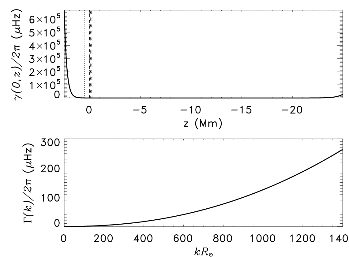
Waves in the Sun are attenuated by granulation and have a finite lifetime. We model the frequency full width at half maximum of the f-mode power using , where Hz and (Gizon and Birch, 2002). The LHS of Equation (\iref\thearticleeqn:F) uses , whereas Gizon and Birch (2002) use . Therefore, the attenuation coefficient used in our equation of motion is half of that used in Gizon and Birch (2002). The full form of the damping, , shown in Figure \iref\thearticlesponge, is given by
The top damping layer introduces a frequency dependence to the eigenmode solutions. High frequency waves have significant energy in the vicinity of the top damping layer and are affected more than the low frequency waves that have less energy at these heights. Any damping layers will affect the eigenfrequencies and lifetimes of the mode, but in this case the lifetimes are predominantly dictated by . The parameters for the damping layers were guesses which were shown to empirically damp the reflected waves sufficiently and not noticeably affect the eigenfrequencies or lifetimes of the modes. The damping layer parameters are not optimised and other forms have also been found to work (Hanasoge, Duvall, and Couvidat, 2007, e.g.). By using the boundary value problem (BVP) solver in Appendix \iref\thearticleapp2 we find that the difference in the eigenfrequencies between having and not having the sponge layers is less than for the f, p1, and p2 modes and a little higher for the p3 and p4 modes (see Appendix \iref\thearticleapp3, Figure \iref\thearticlebvpfigd). If we adjust the range of the top damping layer to Mm we see a maximum 0.5% reduction but only for the p4-modes at high frequencies (see Appendix \iref\thearticleapp3, Figure \iref\thearticlebvpfigf).
2.4 Initial Background Model
We begin with Model S as our background model (starting from any other standard solar model would also be possible). Model S extends to 0.5 Mm above the surface, however our computational domain extends up to 2.5 Mm so that the boundary conditions are sufficiently far from the surface. We extend Model S above Mm in the following way:
| (5) | |||||
| (6) | |||||
| (7) |
where the subscript “S” refers to Model S, the subscript “0” is the extended model. The denominators in the exponents are the scale heights of the density and pressure respectively at . The only requirement for the extension of the background was that it should not increase the wavespeed since we aim to damp the waves at these heights to minimise reflection. Thus, the sound speed was held constant and the pressure and density smoothly extended. The extension is not meant to represent a realistic solar chromosphere and at this height the waves will be artificially damped to prevent reflection.
2.5 Conditions for Convective Stability
convecstab
We want to simulate perturbations superimposed on a background model assuming that the evolution is linear. Part of Model S, and therefore the extended Model S described above, is super-adiabatically stratified and convectively unstable. This instability is a real property of the Sun resulting in modes that, in a linear calculation, grow exponentially in time and will eventually dominate the solution. Therefore, we stabilise the background model against convection to satisfy the condition . We do this by altering the pressure gradient. The reason for choosing to modify the pressure gradient is that it affects the eigenmodes of the model less than changes to the sound speed and/or density (Cameron, Gizon, and Duvall, 2008). We set the pressure gradient in the stabilised model as:
where cgs (at the surface this is ). This formulation was arrived at by empirically testing the stability of the simulation with small values of . An additional constraint was that it should also remain stable with an embedded perturbation (Cameron, Gizon, and Duvall, 2008, e.g. a sunspot as in ). This was the smallest value that was found to satisfy these conditions. The derivatives, here, are evaluated numerically as
| and | ||||
to achieve a greater numerical accuracy. We have tested that this criterion is effective in maintaining stability for simulations for up to ten solar days.
The stabilisation forfeits hydrostatic equilibrium and introduces gravity modes into the solution. The gravity modes all have low frequencies and can easily be excluded from any subsequent analyses. The lack of hydrostatic equilibrium is likely to be more consequential. There are different formulations of the oscillation equations, those that incorporate the assumption of hydrostatic equilibrium and those that do not. We stress that everything presented in this article applies to the formulation presented in Equation \iref\thearticleeqn:F which was derived from the equations of continuity, energy and motion, respectively
(where the primed quantities are the perturbations), without assuming hydrostatic equilibrium. Also, the implications for seismic reciprocity (Dahlen and Tromp, 1998) have not been explored and may be important.
3 Strategy Outline
secstrategy
Now that we have set out the problem, we outline the strategy involved in developing the convectively stable background models presented in this article. It is described as follows:
- •
Begin with Extended Solar Model S.
- •
Convectively stabilise it by changing as described in Section \iref\thearticleconvecstab. This results in CSM.
- •
Compare the eigenfrequencies and eigenfunctions to those of Model S.
- •
We find that the eigenfunctions near the surface, where we are most interested in modelling, are not well matched and the eigenfrequencies have increased.
We are left with the choice to modify the sound speed and/or the density to try to correct the eigenmodes. Since modifying the density has a large effect on the f-mode energy density, we choose to change the sound speed only. Empirically, we found that increasing the sound speed near the surface improves the eigenfunctions:
- •
Begin with Extended Solar Model S.
- •
Increase the sound speed in the top 1 Mm by 10% (Equation \iref\thearticlecsa).
- •
Convectively stabilise the model. This results in CSM_A.
- •
Compare the eigenfrequencies and eigenfunctions to those of Model S.
- •
We find that the eigenfunctions are a better match with Model S than CSM and the eigenfrequencies are only slightly over-estimated.
We attempt to correct the eigenfrequencies by introducing a small decrease in sound speed in the top Mm, which will reduce the overall speed of the waves and thus reduce the eigenfrequencies:
- •
Begin with Extended Solar Model S.
- •
Take the sound speed profile of CSM_A and introduce an additional decrease in the sound speed of 3% in the top Mm (Equation \iref\thearticlecsb).
- •
Convectively stabilise the model.
- •
Compare the eigenfrequencies and eigenfunctions to those of Model S.
- •
We find the eigenfrequencies are closer to Model S and the eigenfunctions are only moderately further from Model S than CSM_A. This results in CSM_B.
For a smooth transition, a Gaussian function was selected for the sound speed changes. The particular parameters were determined by trial-and-error of a few guesses to empirically evaluate how they further affected the eigenmodes. The comparisons to the eigenmodes of Model S were judged by eye. We calculated the eigenmodes of the models in two ways. The first used the SLiM numerical simulations (see Appendix \iref\thearticleapp1) and the second used a BVP solver (see Appendix \iref\thearticleapp2).
As a quantitative measure of the difference between eigenfrequencies of Model S and the featured models, we compute the relative difference of the real part of the eigenfrequencies (determined from both SLiM and the BVP) to the real part of the Model S eigenfrequencies, . These particular Model S eigenfrequencies were calculated as in Birch, Kosovichev, and Duvall (2004) using a Cartesian geometry and constant gravity. For the modes we are interested in, the geometry and radially dependent gravity affect the eigenfrequencies by no more than 0.5% (see Appendix \iref\thearticleapp3). We measure the difference between the eigenfunctions of Model S and the stabilised model in two ways. The first, by calculating the relative difference in area under near the surface between Model S and the respective stabilised model. The second, by calculating the difference of the height [] of the uppermost peak of between Model S and the respective stabilised model for each eigenmode (Section \iref\thearticlesl).
4 Convectively Stable Model (CSM)
seccsm Figure \iref\thearticlecsm shows the relative difference between the stabilised pressure gradient of CSM and the pressure gradient of Model S, , which is as large as 35% near the surface. We now discuss the effect this change in the pressure gradient has on the eigenmodes.
Figure \iref\thearticlenocs_efunc shows , normalised so that , as a function of for f and p1 to p4 eigenmodes from Model S and CSM (derived using both SLiM and the BVP). Recall that the depth of our domain allows us to study only up to the p4 mode. The horizontal velocity component of the eigenfunctions, , was found to have a similar agreement with Model S.
We observe that the main effect of the stabilisation on the eigenfunctions is to decrease the amplitude of near the surface. Since this is where the stabilisation has the greatest effect on the pressure gradient, changes to the eigenfunctions in this region are not unexpected.
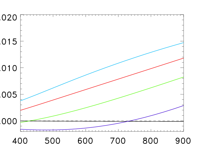
Figure \iref\thearticlecsmp shows the relative difference of the real part of the eigenfrequencies, , for each radial order as a function of wavenumber. The quantitative average over shows that the increase in the eigenfrequencies is less than 2%. The increase in f-mode eigenfrequencies compared to Model S can be attributed to the treatment of gravity and geometry of the operators (see Appendix \iref\thearticleapp3). The agreement between Model S and each of the convectively stable models will be quantified in Section \iref\thearticlesl.
Since it is a necessity to modify Model S, and therefore no subsequent model will have exactly the same eigenmodes, we attempt to correct the eigenmodes by modifying the sound speed. We found a trade-off between having eigenfunctions or eigenfrequencies closer to those of Model S. In model CSM_A (Section \iref\thearticleseccsma) we attempt to improve the eigenfunctions and in CSM_B we try to improve the eigenfrequencies without affecting the eigenfunctions too much (Section \iref\thearticleseccsmb).


5 Convectively Stable Model A (CSM_A)
seccsma
We follow the procedure set out in Section \iref\thearticlesecstrategy. We found that an increase in sound speed improved the match between the eigenfunctions of CSM and Model S near the surface. We chose
| (8) |
where the subscript “A” indicates CSM_A. Starting from Model S with specifying the sound speed, we then rederived the pressure gradient required for stability as set out in Section \iref\thearticleconvecstab. Figure \iref\thearticlesmsa shows the relative difference between CSM_A and Model S of the sound speed squared and the pressure gradient as a function of height. This change in sound speed was found to raise the height of the uppermost peak of . Figure \iref\thearticlesmsa_efunc shows for various eigenmodes from CSM_A for each radial order, f and p1 to p4. Particularly, the f-mode eigenfunctions are close to Model S. The p1 and p2 modes are also a better match, especially near the surface.
The real parts of the eigenfrequencies, shown in Figure \iref\thearticleefreqa, are not significantly affected: the average (over ) relative difference for each radial order is still less than 2% of Model S values. We have constructed a convectively stable model, CSM_A, with eigenfunctions closer to Model S than CSM and reasonably similar eigenfrequencies.


6 Convectively Stable Model B (CSM_B)
seccsmb
Starting from Model S and , we constructed a model with eigenfrequencies closer to Model S than CSM_A and reasonable eigenfunctions (as described in Section \iref\thearticlesecstrategy). The eigenfrequencies are related to the phase speed of the wave () and so we slowed the waves down by adding a broad reduction in sound speed of CSM_A. We chose
| (9) |
where subscript “B” indicates CSM_B. Figure \iref\thearticlesmsb shows the relative difference between CSM_B and Model S (a) sound speed squared and (b) pressure gradient as a function of height.

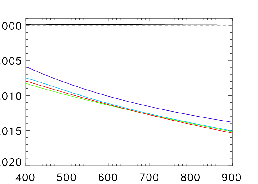
The eigenfunctions are slightly adversely affected as can be seen by comparing Figure \iref\thearticlesmsb_efunc with Figure \iref\thearticlesmsa_efunc, however they are still more solar-like than those of CSM (Figure \iref\thearticlenocs_efunc). The real parts of the eigenfrequencies (Figure \iref\thearticleefreqb) reduce to within 1% of Model S. We have not found a model which resulted in more similar eigenfrequencies without grossly changing the eigenfunctions. With this sound speed profile, we have arrived at a convectively stable model, CSM_B, with eigenfrequencies closer to those of Model S than CSM or CSM_A.


7 Comparison of Eigenfunctions
sl
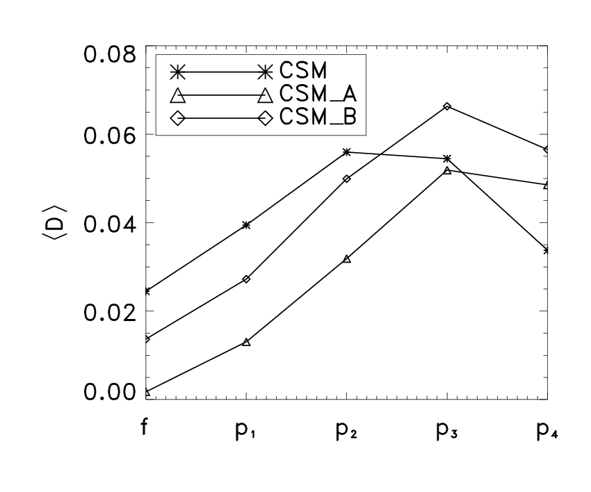
Quantitatively, we compare the eigenfunctions by finding the relative difference of the area under between Model S and each convectively stable background in the near-surface layers, Mm. The difference is defined by
| (10) |
This integration range was chosen because this is where the stabilisation has greatest effect. For each radial order we take the mean of over , giving a quantitative measure of the differences between the eigenfunctions of Model S and the stabilised model []. Figure \iref\thearticleavec shows that for the f, p1 and p2 modes CSM_A (triangle) has eigenfunctions closest to that of Model S, while CSM (asterisk) has those farthest from Model S.
avec

In addition, we measure the height of the uppermost peak, , of . Figure \iref\thearticlepken shows for each radial order and each model as indicated. From this we see that stabilising the background causes to drop in height (i.e. the difference between the solid and the long-dash curves). Increasing the sound speed in a narrow region close to the surface (CSM_A) pushes the peak back towards the surface (dotted curves). The broad decrease in sound speed added in CSM_B does not change the location of the peak too much (short-dash curves). The sudden transition to very high upper turning points at high wavenumber for Model S (particularly for the p1 and p2 modes) is due to the protuberance in the Model S eigenfunctions very close to the surface (for example, the f and p1-modes in Figure \iref\thearticlenocs_efunc) which is absent in the stable models. The protuberance is due to rapid changes in the density scale height close to the surface that disappears after the stabilisation (reduction of ).
We now have three convectively stable solar models each having similar, but slightly different, eigenfrequencies and eigenfunctions to Model S. Having models focused on achieving slight variations of the same goal (more similar eigenfunctions or eigenfrequencies) gives us the possibility of testing the sensitivity of helioseismic analysis techniques to the background properties.
8 Modelling the Random Wave Field
8.1 Random wave excitation model
rwem We model the random wave excitation by imposing a vertical force, , to the right-hand-side of Equation (\iref\thearticleeqn:F). The force is specified by
| (11) |
where is a horizontal wavevector, is an angular frequency, Mm is the width of the source, and the acceleration is a realisation of a complex Gaussian random variable with zero mean and variance where mHz (Gizon and Birch, 2004). The height of the sources is at Mm, which is close to the highly superadiabatic layer where solar waves are expected to be strongly excited (Nigam and Kosovichev, 1999). In reality, the sources in the Sun will also have a wavenumber dependence which we have not included. In practice, the sources are generated before the simulation commences and saved with a 30 second cadence. The forcing is applied at each time step (in cases herein this is approximately 0.13 solar seconds), with the value of the applied forcing changing every 30 solar seconds. We remark that we first tried to use a Lorentzian for the frequency dependence (Title et al., 1989; Gizon and Birch, 2002), corresponding to sources which decay exponentially in time. We found that the resulting power was too strong at high frequencies compared with observations, and that the Gaussian distribution produced a better agreement.
8.2 Azimuthally Averaged Power Spectra
In this section we used SLiM to investigate the response of CSM_A and CSM_B to the random wave excitation model as described in Section \iref\thearticlerwem. A total of 16 hours was simulated, however the first eight hours, during which the wave field is reaching a steady state, are discarded. To mimic SOHO/MDI observations, we save vertical-velocity data at a height of 0.2 Mm above the surface (the height at which SOHO/MDI observes, see Bruls (1993)) and account for the modulation transfer function of the instrument by multiplying the simulated power spectra by the modulation transfer function of Rabello-Soares, Korzennik, and Schou (2001).
To make a comparison with an observed power spectra, we took eight hours of Postel projected (centred at a longitude of and latitude of ) full-disk Doppler observations with a 60 second cadence from SOHO/MDI on 21 January 2002. The observations consist primarily of quiet Sun covering a surface area identical to the simulations.
We consider the azimuthally averaged (with bin size Mm]) power spectra of the observations, , and of the simulations with CSM_A and CSM_B, are shown in Figures \iref\thearticleOBSSPECTRA, \iref\thearticleASPECTRA, and \iref\thearticleBSPECTRA respectively. The dashed curves are the eigenfrequencies calculated from Model S for comparison. The straight solid line is where is equal to and Mm; as stated previously, modelling a higher would require a deeper box. There is some power evident in the low frequencies which are most likely g-modes introduced by stabilising the background. These are the artificial product of having a stable model. Thus, this region cannot be compared to solar observations. The remaining “comparable domain”: where is the lower curve shown in these figures, should contain modes which are comparable to those on the Sun. The azimuthally averaged power spectra are normalised to the mean power within a region defined by . By inspection, the power spectra of CSM_A (Figure \iref\thearticleASPECTRA) and CSM_B (Figure \iref\thearticleBSPECTRA) look qualitatively similar to the observed spectrum (Figure \iref\thearticleOBSSPECTRA). We now take a closer look at the properties.


8.3 Amplitudes of the Power Spectra
Figure \iref\thearticlepcut shows vertical cuts through the power spectra in Figures \iref\thearticleOBSSPECTRA, \iref\thearticleASPECTRA, and \iref\thearticleBSPECTRA as a function of frequency. The Model S eigenfrequencies (vertical lines) are larger than those of the observations (solid curve), while CSM_A (dash curve) and CSM_B (dot curve) eigenfrequencies are larger than those of Model S. It also shows that the maximum power and linewidths of the ridges agree with observations best at low frequency.

Figure \iref\thearticlepave shows the total power in the comparable range for the observations (solid curve), CSM_A (dash curve) and CSM_B (dot curve) as a function of (a) frequency and (b) . The maximum power in the simulations occurs at a larger wavenumber than in the observational power. Correcting this could be done by fine tuning the wave excitation model, and may be done in the future, however the results presented here are sufficiently close for a large number of studies.

8.4 Fitting the Power Spectra
We analyse the properties of the azimuthally averaged power spectra in Figures \iref\thearticleOBSSPECTRA, \iref\thearticleASPECTRA and \iref\thearticleBSPECTRA by fitting asymmetric Lorentzians (Duvall et al., 1993; Gizon, 2006, e.g.),
| (12) | |||
to cuts at fixed wavenumber as a function of frequency. In Equation (\iref\thearticlealor), the maximum power of the ridge is given by and is located at a frequency , the valley is at , the noise is , and the full-width-at-half-maximum (FWHM) of the asymmetric Lorentzian is . The fitting is done using a Levenberg-Marquardt algorithm for least squares curve fitting using the IDL mpfit package. The frequency range of the fit is from of the f-mode Model S eigenfrequency to of the p4-mode Model S eigenfrequency. We define the asymmetry parameter as (Gizon, 2006).

Figure \iref\thearticlepower shows the maximum power of each from fitting Equation (\iref\thearticlealor) to the power spectrum of the observations (top), CSM_A (middle) and CSM_B (bottom). The simulated power spectra have stronger power at high frequency than the observations. In addition, the maximum power of occurs at a lower frequency in the simulations than in the observations.

Figure \iref\thearticlefwhm shows the FWHM of the Lorentzian fit for each mode in the power spectrum of the observations (top), CSM_A (middle) and CSM_B (bottom). The FWHM of the ridges in the observations is consistent with Figure 2 in Antia and Basu (1999), keeping in mind that these are coarse measurements. The simulation ridges have larger FWHMs than the observations for f and p1 modes.

Figure \iref\thearticlefreq shows the relative difference of the central ridge frequencies to Model S for the observations (top), CSM_A (middle) and CSM_B (bottom). The results from the Lorentzian fitting are within 1% of the BVP solutions as shown in Figure \iref\thearticlefreqcomp.


Figure \iref\thearticlechi shows the asymmetries of the observations (top), CSM_A (middle) and CSM_B (bottom). We achieve the correct sign and comparable magnitude of the asymmetry for all the modes. The f-mode has negative asymmetries, and the value of the asymmetries increases with increasing mode number which is in agreement with Gizon (2006).
We have demonstrated the response of the numerical simulations of wave excitation in the Sun using two of the convectively stable background models, CSM_A and CSM_B. The eigenmodes of the background models and the parameters of the sources of acoustic wave oscillations are sufficient to be used as a foundation for quantitative solar-like simulations.
In addition, we have successfully implemented the stable background models into the framework of another code which also computes linear simulations of helioseismic wave propagation, the Seismic Propagation through Active Regions and Convection (SPARC) code (Hanasoge et al., 2006; Hanasoge, Duvall, and Couvidat, 2007).
9 Discussion
We have created three convectively stable solar models which, to slightly differing extents, have similar eigenmodes to those of Model S. We have also computed helioseismic simulations using a model for the random excitation of waves, which together with the stable solar models, reproduce the SOHO/MDI observed mode frequencies and asymmetries well for each of the f and p1 to p4 ridges. The linewidths of the ridges and the power distribution are reasonably similar to those of the Sun.
Although stabilising the background model is an important step in numerical studies of wave propagation (Parchevsky and Kosovichev, 2007; Cameron, Gizon, and Duvall, 2008; Shelyag, Fedun, and Erdélyi, 2008; Schunker, Cameron, and Gizon, 2010, and has been done before, e.g. by), its effects on the eigenfunctions and eigenfrequencies has received little attention. An optimal way to produce a convectively stable background model for numerical simulations has not been formulated, but nevertheless the models presented here should be useful for a range of studies. In particular, we envisage that these models will be used to study the propagation of solar waves through three-dimensional heterogeneities, such as convective flows, granulation and model sunspots (Cameron et al., 2011; Dombroski, Birch, and Braun, 2011, e.g.). Having three models with slightly different properties will enable us to quantitatively test the sensitivity of the results to the details of the models. The models and extra information from the analysis in this paper are available for download from the HELAS local helioseismology website (Schunker and Gizon, 2008, http://www.mps.mpg.de/projects/seismo/NA4/;).
Appendix A Calculating Eigenmodes Using Simulations
app1 The following procedure calculates the eigenmodes of the system using SLiM and is designed to be applied iteratively. We began by simulating the response of the system to a wave packet constructed from Model S eigenmodes of one radial order (as in Cameron, Gizon, and Duvall, 2008). The outputs, and , of a five hour long simulation were saved with a one minute cadence. We then took the Fourier transform of the velocity field in time, . From this we determined the eigenfrequencies from a linear fit in time to the phase with the wrap-around removed. The function we used to fit the phase, , is given by . The height of 200 km corresponds to the observation height of SOHO/MDI (Bruls, 1993). We determined the radial component by applying a broad ridge filter to isolate the appropriate radial order, centred on the improved (subscript ) estimate of the real part of the eigenfrequencies . The same filter was applied to the horizontal velocity to get . The velocities are then Fourier transformed from frequency space back to time.
The improved eigenmodes are then given by
Note that and the denominator are defined from the vertical velocity component, at km. From these eigenmodes we constructed a new wave packet initial condition and the simulation was re-computed with this wave packet. In practice we found that a single pass is sufficient and the improved eigenmodes from the first simulation were used to compare to Model S.
Appendix B Determining the Eigenmodes of the Boundary Value Problem
app2
The perturbations of a particular eigenmode with radial order of the Equation (\iref\thearticleeqn:F) have the form
| (13) | |||||
| (14) |
with .
After some manipulation (using the continuity equation, equation of motion and energy equation), our system of equations becomes
| (15) | |||
| (16) |
where .
Following the method of Birch, Kosovichev, and Duvall (2004), we substitute
into Equations (\iref\thearticlef1) and (\iref\thearticlef2) to get
| (17) |
and
| (18) |
Then multiplying Equation (\iref\thearticley2s) by and Equation (\iref\thearticley1s) by and rearranging, we get
| (19) |
and
| (20) |
where and . Equation (\iref\thearticleeighteen) and (\iref\thearticlenineteen) reduce to Equations (A10) and (A11) in Birch, Kosovichev, and Duvall (2004) in the case where the attenuation is not dependent on , the background is in hydrostatic equilibrium and the geometry is Cartesian.
The top boundary condition is a free surface such that the Lagrangian pressure perturbation [] is zero. This means that . The bottom boundary is specified by and . The boundary conditions translated to and are that at the top and and at the bottom.
We solve this boundary value problem using the Matlab program bvp4c. In order to be consistent with the eigenfunction solutions from the SLiM simulations, we do a similar normalisation of the eigenfunctions so that .
Appendix C Solutions to the BVP for Different Background Models
app3 We use the BVP solver outlined in Appendix \iref\thearticleapp2 to explore the effects on the eigenfrequencies by changing different parameters of the problem with CSM_A. To test the robustness of the BVP solver we added 1% noise to the eigenfrequency guess that results in a relative difference of less than as shown in Figure \iref\thearticlebvpfig (a). In Figure \iref\thearticlebvpfig (b) we do not apply any wave attenuation, i.e. . The eigenfrequencies decrease in value compared to the CSM_A eigenfrequencies, more so for the higher order modes. In Figure \iref\thearticlebvpfig (c) we have set a constant gravitational acceleration of . This mostly affects the f-mode, but the eigenfrequencies are also decreased for the p-modes. Removing the sponge layers, so that , give results, Figure \iref\thearticlebvpfig (d), that are similar to (b). Using the full Cartesian operators, as opposed to the spherical derivative in the radial direction as in Equation \iref\thearticleeqn:A2, affects the eigenfrequencies at low-wavenumber the greatest, as shown in Figure \iref\thearticlebvpfig (e). In Figure \iref\thearticlebvpfig (f) we have lowered the top damping layer to have Hz for Mm (retaining the bottom damping layer), which decreases the eigenfrequencies. These frequency shifts are small compared to the frequency shifts caused by the convectively stabilising the models.

\acknowledgementsname
This work is supported by ERC grant agreement 210949, “Seismic Imaging of the Solar Interior”, to PI L. Gizon (Milestone #4). We thank Aaron Birch for providing a set of Model S eigenmodes, Shravan Hanasoge for the SPARC code, and Cristina Rabello-Soares for the full-disk MDI point spread function. SOHO is a mission of international collaboration between ESA and NASA.
References
- Antia and Basu (1999) Antia, H.M., Basu, S.: 1999, High-Frequency and High-Wavenumber Solar Oscillations. ApJ 519, 400 – 406. doi:10.1086/307364.
- Birch, Kosovichev, and Duvall (2004) Birch, A.C., Kosovichev, A.G., Duvall, T.L. Jr.: 2004, Sensitivity of Acoustic Wave Travel Times to Sound-Speed Perturbations in the Solar Interior. ApJ 608, 580 – 600. doi:10.1086/386361.
- Bruls (1993) Bruls, J.H.M.J.: 1993, The formation of helioseismology lines. IV - The NI I 676.8 NM intercombination line. A&A 269, 509 – 517.
- Cally and Bogdan (1993) Cally, P.S., Bogdan, T.J.: 1993, Solar p-modes in a vertical magnetic field - Trapped and damped pi-modes. ApJ 402, 721 – 732. doi:10.1086/172172.
- Cameron, Gizon, and Daiffallah (2007) Cameron, R., Gizon, L., Daiffallah, K.: 2007, SLiM: a code for the simulation of wave propagation through an inhomogeneous, magnetised solar atmosphere. Astronom. Nach. 328, 313. doi:10.1002/asna.200610736.
- Cameron, Gizon, and Duvall (2008) Cameron, R., Gizon, L., Duvall, T.L. Jr.: 2008, Helioseismology of Sunspots: Confronting Observations with Three-Dimensional MHD Simulations of Wave Propagation. Sol. Phys. 251, 291 – 308. doi:10.1007/s11207-008-9148-1.
- Cameron et al. (2011) Cameron, R., Schunker, H., Gizon, L., Pietarila, A.: 2011, Semi-empirical sunspot models for helioseismology. Sol. Phys. 268, 293 – 308. doi:10.1007/s11207-010-9631-3.
- Christensen-Dalsgaard et al. (1996) Christensen-Dalsgaard, J., Dappen, W., Ajukov, S.V., Anderson, E.R., Antia, H.M., Basu, S., Baturin, V.A., Berthomieu, G., Chaboyer, B., Chitre, S.M., Cox, A.N., Demarque, P., Donatowicz, J., Dziembowski, W.A., Gabriel, M., Gough, D.O., Guenther, D.B., Guzik, J.A., Harvey, J.W., Hill, F., Houdek, G., Iglesias, C.A., Kosovichev, A.G., Leibacher, J.W., Morel, P., Proffitt, C.R., Provost, J., Reiter, J., Rhodes, E.J. Jr., Rogers, F.J., Roxburgh, I.W., Thompson, M.J., Ulrich, R.K.: 1996, The Current State of Solar Modeling. Science 272, 1286 – 1292.
- Dahlen and Tromp (1998) Dahlen, F.A., Tromp, J.: 1998, Theoretical global seismology, Princeton University Press, Princeton, New Jersey, 120.
- Dombroski, Birch, and Braun (2011) Dombroski, D., Birch, A., Braun, D.: 2011, Testing Helioseismic Holography Inversions for Supergranular Flows Using Synthetic Data. Sol. Phys., in prep.
- Duvall et al. (1993) Duvall, T.L. Jr., Jefferies, S.M., Harvey, J.W., Osaki, Y., Pomerantz, M.A.: 1993, Asymmetries of solar oscillation line profiles. ApJ 410, 829 – 836. doi:10.1086/172800.
- Gizon (2006) Gizon, L.: 2006, Line Profiles of Fundamental Modes of Solar Oscillation. Central Euro. Astrophys. Bull. 30, 1 – 9.
- Gizon and Birch (2002) Gizon, L., Birch, A.C.: 2002, Time-Distance Helioseismology: The Forward Problem for Random Distributed Sources. ApJ 571, 966 – 986. doi:10.1086/340015.
- Gizon and Birch (2004) Gizon, L., Birch, A.C.: 2004, Time-Distance Helioseismology: Noise Estimation. ApJ 614, 472 – 489. doi:10.1086/423367.
- Hanasoge, Duvall, and Couvidat (2007) Hanasoge, S.M., Duvall, T.L. Jr., Couvidat, S.: 2007, Validation of Helioseismology through Forward Modeling: Realization Noise Subtraction and Kernels. ApJ 664, 1234 – 1243. doi:10.1086/519070.
- Hanasoge et al. (2006) Hanasoge, S.M., Larsen, R.M., Duvall, T.L. Jr., De Rosa, M.L., Hurlburt, N.E., Schou, J., Roth, M., Christensen-Dalsgaard, J., Lele, S.K.: 2006, Computational Acoustics in Spherical Geometry: Steps toward Validating Helioseismology. ApJ 648, 1268 – 1275. doi:10.1086/505927.
- Lynden-Bell and Ostriker (1967) Lynden-Bell, D., Ostriker, J.P.: 1967, On the stability of differentially rotating bodies. MNRAS 136, 293.
- Nigam and Kosovichev (1999) Nigam, R., Kosovichev, A.G.: 1999, Source of Solar Acoustic Modes. ApJ 514, L53 – L56. doi:10.1086/311939.
- Parchevsky and Kosovichev (2007) Parchevsky, K.V., Kosovichev, A.G.: 2007, Three-dimensional Numerical Simulations of the Acoustic Wave Field in the Upper Convection Zone of the Sun. ApJ 666, 547 – 558. doi:10.1086/520108.
- Rabello-Soares, Korzennik, and Schou (2001) Rabello-Soares, M.C., Korzennik, S.G., Schou, J.: 2001, The determination of MDI high-degree mode frequencies. In: Pallé, W.. (ed.) SOHO 10/GONG 2000 Workshop: Helio- and Asteroseismology at the Dawn of the Millennium SP-464, ESA, Nordwijk, 129 – 136.
- Scherrer et al. (1995) Scherrer, P.H., Bogart, R.S., Bush, R.I., Hoeksema, J.T., Kosovichev, A.G., Schou, J., Rosenberg, W., Springer, L., Tarbell, T.D., Title, A., Wolfson, C.J., Zayer, I., MDI Engineering Team: 1995, The Solar Oscillations Investigation - Michelson Doppler Imager. Sol. Phys. 162, 129 – 188. doi:10.1007/BF00733429.
- Schunker and Gizon (2008) Schunker, H., Gizon, L.: 2008, HELAS Local Helioseismology Activities. Comm. in Asteroseis. 156, 93 – 105.
- Schunker, Cameron, and Gizon (2010) Schunker, H., Cameron, R., Gizon, L.: 2010, Convectively stabilised background solar models for local helioseismology. ArXiv e-prints: 1002.1969.
- Shelyag, Fedun, and Erdélyi (2008) Shelyag, S., Fedun, V., Erdélyi, R.: 2008, Magnetohydrodynamic code for gravitationally-stratified media. A&A 486, 655 – 662. doi:10.1051/0004-6361:200809800.
- Title et al. (1989) Title, A.M., Tarbell, T.D., Topka, K.P., Ferguson, S.H., Shine, R.A., SOUP Team: 1989, Statistical properties of solar granulation derived from the SOUP instrument on Spacelab 2. ApJ 336, 475 – 494. doi:10.1086/167026.