Consistency of Functional Learning Methods Based on Derivatives

We consider a pair of random variables $(X,Y)$ where $X$ takes values in a functional space $\cal X$ and $Y$ is either a real valued random variable (regression case) or a random variable taking values in $\{-1,1\}$ (binary classification case). From this, we are given a learning set $S_{n}=\{(X_{i},Y_{i})\}_{i=1}^{n}$ of $n$ independent copies of $(X,Y)$. Moreover, the functions $X_{i}$ are not entirely known but sampled according to a non random sampling grid of finite length, $\tau_{d}=(t_{l})_{l=1}^{|\tau_{d}|}$: we only observe $\mathbf{X}^{\tau_{d}}_{i}=(X_{i}(t_{1}),\ldots X_{i}(t_{|\tau_{d}|}))^{T}$, a vector of $\mathbb{R}^{|\tau_{d}|}$ and denote $S_{n,\tau_{d}}$ the corresponding learning set. Our goal is to construct:

1. 1.

   in the binary classification case: a classifier, $\phi_{n,\tau_{d}}$, whose misclassification probability

   $$L(\phi_{n,\tau_{d}})=\mathbb{P}\left(\phi_{n,\tau_{d}}(\mathbf{X}^{\tau_{d}})\neq Y\right)$$

   asymptotically reaches the Bayes risk

   $$L^{*}=\inf_{\phi:{\cal X}\rightarrow\{-1,1\}}\mathbb{P}\left(\phi(X)\neq Y\right)$$

   i.e., $\lim_{|\tau_{d}|\rightarrow+\infty}\lim_{n\rightarrow+\infty}\mathbb{E}\left(L(\phi_{n,\tau_{d}})\right)=L^{*}$ ;

2. 2.

   in the regression case: a regression function, $\phi_{n,\tau_{d}}$, whose $L^{2}$ error

   $$L(\phi_{n,\tau_{d}})=\mathbb{E}\left([\phi_{n,\tau_{d}}(\mathbf{X}^{\tau_{d}})-Y]^{2}\right)$$

   asymptotically reaches the minimal $L^{2}$ error

   $$L^{*}=\inf_{\phi:{\cal X}\rightarrow\mathbb{R}}\mathbb{E}\left([\phi{}(\mathbf{X}^{\tau_{d}})-Y]^{2}\right)$$

   i.e., $\lim_{|\tau_{d}|\rightarrow+\infty}\lim_{n\rightarrow+\infty}L(\phi_{n,\tau_{d}})=L^{*}$.

   This definition implicitly requires $\mathbb{E}\left(Y^{2}\right)<\infty$ and as a consequence, corresponds to a $L^{2}$ convergence of $\phi_{n,\tau_{d}}$ to the conditional expectation $\phi^{*}=\mathbb{E}\left(Y|X\right)$, i.e., to $\lim_{|\tau_{d}|\rightarrow+\infty}\lim_{n\rightarrow+\infty}\mathbb{E}\left([\phi_{n,\tau_{d}}(\mathbf{X}^{\tau_{d}})-\phi^{*}(X)]^{2}\right)=0$.

Such $\phi_{n,\tau_{d}}$ are said to be (weakly) consistent Devroye et al. (1996); Györfi et al. (2002). We have deliberately used the same notations for the (optimal) predictive performances in both the binary classification and the regression case. We will call $L^{*}$ the Bayes risk even in the case of regression. Most of the theoretical background of this paper is common to both the regression case and the classification case: the distinction between both cases will be made only when necessary.

As pointed out in the introduction, the main difficulty is to show that the performances of a model built on the $\mathbf{X}^{\tau_{d}}_{i}$ asymptotically reach the best performance achievable on the original functions $X_{i}$. In addition, we will build the model on derivatives estimated from the $\mathbf{X}^{\tau_{d}}_{i}$.

Our goal is to leverage the functional nature of the data by allowing differentiation operators to be applied to functions prior their submission to a more common classifier or regression function. Therefore we assume that the functional space $\cal X$ contains only differentiable functions. More precisely, $\cal X$ is the Sobolev space $\mathcal{H}^{m}=\Bigl\{h\in L^{2}([0,1])\mid\,\forall\,j=1,\ldots,m,\ D^{j}h\text{ exists in the weak sense,}\,\text{and }D^{m}h\in L^{2}([0,1])\Bigr\}$, where $D^{j}h$ is the $j$-th derivative of $h$ (also denoted by $h^{(j)}$) and for an integer $m\geq 1$. Of course, by a straightforward generalization, any bounded interval can be considered instead of $[0,1]$.

To estimate the underlying functions $X_{i}$ and their derivatives from sampled data, we rely on smoothing splines. More precisely, let us consider a deterministic function $x\in\mathcal{H}^{m}$ sampled on the aforementioned grid. A smoothing spline estimate of $x$ is the solution, $\widehat{x}_{\lambda,\tau_{d}}$, of

where $\lambda$ is a regularization parameter that balances interpolation error and smoothness (measured by the $L^{2}$ norm of the $m$-th derivative of the estimate). The goal is to show that a classifier or a regression function built on $\widehat{X}_{\lambda,\tau_{d}}^{(m)}$ is consistent for the original problem (i.e., the problem defined by the pair $(X,Y)$): this means that using $\widehat{X}_{\lambda,\tau_{d}}^{(m)}$ instead of $X$ has no dramatic consequences on the accuracy of the classifier or of the regression function. In other words, asymptotically, no information loss occurs when one replaces $X$ by $\widehat{X}_{\lambda,\tau_{d}}^{(m)}$.

The proof is based on the following steps:

1. 1.

   First, we show that building a classifier or a regression function on $\widehat{X}_{\lambda,\tau_{d}}^{(m)}$ is approximately equivalent to building a classifier or a regression function on $\mathbf{X}^{\tau_{d}}=(X(t_{l}))_{l=1}^{|\tau_{d}|}$ using a specific metric. This is done by leveraging the Reproducing Kernel Hilbert Space (RKHS) structure of $\mathcal{H}^{m}$. This part serves one main purpose: it provides a solution to work with estimation of the derivatives of the original function in a way that preserves all the information available in $\mathbf{X}^{\tau_{d}}$. In other words, the best predictive performances for $Y$ theoretically available by building a multivariate model on $\mathbf{X}^{\tau_{d}}$ are equal to the best predictive performances obtained by building a functional model on $\widehat{X}_{\lambda,\tau_{d}}^{(m)}$.

2. 2.

   Then, we link $\mathbb{E}\left(Y|\widehat{X}_{\lambda,\tau_{d}}\right)$ with $\mathbb{E}\left(Y|X\right)$ by approximation results available for smoothing splines. This part of the proof handles the effects of sampling.

3. 3.

   Finally, we glue both results via standard $\mathbb{R}^{|\tau_{d}|}$ consistency results.

As we want to work on derivatives of functions from $\mathcal{H}^{m}$, a natural inner product for two functions of $\mathcal{H}^{m}$ would be $(u,v)\rightarrow\int_{0}^{1}u^{(m)}(t)v^{(m)}(t)dt$. However, we prefer to use an inner product of $\mathcal{H}^{m}$ ($\int_{0}^{1}u^{(m)}(t)v^{(m)}(t)dt$ only induces a semi-norm on $\mathcal{H}^{m}$) because, as will be shown later, such an inner product is related to an inner product between the sampled functions considered as vectors of $\mathbb{R}^{|\tau_{d}|}$.

This can be done by decomposing $\mathcal{H}^{m}$ into $\mathcal{H}^{m}=\mathcal{H}^{m}_{0}\oplus\mathcal{H}^{m}_{1}$ Kimeldorf and Wahba (1971), where $\mathcal{H}^{m}_{0}=\textrm{Ker}D^{m}=\mathbb{P}^{m-1}$ (the space of polynomial functions of degree less or equal to $m-1$) and $\mathcal{H}^{m}_{1}$ is an infinite dimensional subspace of $\mathcal{H}^{m}$ defined via $m$ boundary conditions. The boundary conditions are given by a full rank linear operator from $\mathcal{H}^{m}$ to $\mathbb{R}^{m}$, denoted $B$, such that $\textrm{Ker}B\cap\mathbb{P}^{m-1}=\{0\}$. Classical examples of boundary conditions include the case of “natural splines” (for $m=2$, $h(0)=h(1)=0$) and constraints that target only the first values of $h$ and its derivatives at a fixed position, for instance the conditions: $h(0)=\ldots=h^{(m-1)}(0)=0$. Other boundary conditions can be used Berlinet and Thomas-Agnan (2004); Besse and Ramsay (1986); Craven and Wahba (1978), depending on the application.

Once the boundary conditions are fixed, an inner product on both $\mathcal{H}^{m}_{0}$ and $\mathcal{H}^{m}_{1}$ can be defined:

is an inner product on $\mathcal{H}^{m}_{1}$ (as $h\in\mathcal{H}^{m}_{1}$ and $D^{m}h\equiv 0$ give $h\equiv 0$). Moreover, if we denote $B=(B^{j})_{j=1}^{m}$, then $\langle u,v\rangle_{0}=\sum_{j=1}^{m}B^{j}uB^{j}v$ is an inner product on $\mathcal{H}^{m}_{0}$. We obtain this way an inner product on $\mathcal{H}^{m}$ given by

where $\mathcal{P}^{m}_{i}$ is the projector on $\mathcal{H}^{m}_{i}$.

Equipped with $\langle.,.\rangle_{\mathcal{H}^{m}}$, $\mathcal{H}^{m}$ is a Reproducing Kernel Hilbert Space (RKHS, see e.g. Berlinet and Thomas-Agnan (2004); Heckman and Ramsay (2000); Wahba (1990)). More precisely, it exists a kernel $k:[0,1]^{2}\rightarrow\mathbb{R}$ such that, for all $u\in\mathcal{H}^{m}$ and all $t\in[0,1]$, $\langle u,k(t,.)\rangle_{\mathcal{H}^{m}}=u(t)$. The same occurs for $\mathcal{H}^{m}_{0}$ and $\mathcal{H}^{m}_{1}$ which respectively have reproducing kernels denoted by $k_{0}$ and $k_{1}$. We have $k=k_{0}+k_{1}$.

In the most common cases, $k_{0}$ and $k_{1}$ have already been explicitly calculated (see e.g., Berlinet and Thomas-Agnan (2004), especially chapter 6, sections 1.1 and 1.6.2). For example, for $m\geq 1$ and the boundary conditions $h(0)=h^{\prime}(0)=\ldots=h^{(m-1)}(0)=0$, we have:

and

We need now to compute to $\widehat{x}_{\lambda,\tau_{d}}$ starting with $\mathbf{x}^{\tau_{d}}=(x(t))_{t\in\tau_{d}}^{T}$. This can be done via a theorem from Kimeldorf and Wahba (1971). We need the following compatibility assumptions between the sampling grid $\tau_{d}$ and the boundary conditions operator $B$:

Then $\widehat{x}_{\lambda,\tau_{d}}$ and $\mathbf{x}^{\tau_{d}}=(x(t))_{t\in\tau_{d}}^{T}$ are linked by the following result:

The first important consequence of Theorem 1 is that building a model on $\widehat{X}_{\lambda,\tau_{d}}$ or on $\mathbf{X}^{\tau_{d}}$ leads to the same optimal predictive performances (to the same Bayes risk). This is formalized by the following corollary:

The second important consequence of Theorem 1 is that the inner product $\langle.,.\rangle_{\mathcal{H}^{m}}$ is equivalent to a specific inner product on $\mathbb{R}^{|\tau_{d}|}$ given in the following corollary:

The corollary is a direct consequence of equations (2) and (3).

In practice, the corollary means that the euclidean space $\left(\mathbb{R}^{|\tau_{d}|},\langle.,.\rangle_{\mathbf{M}_{\lambda,\tau_{d}}}\right)$ is isomorphic to $\left(\mathcal{I}_{\lambda,\tau_{d}},\langle.,.\rangle_{\mathcal{H}^{m}}\right)$, where $\mathcal{I}_{\lambda,\tau_{d}}$ is the image of $\mathbb{R}^{|\tau_{d}|}$ by $\mathcal{S}_{{\lambda},\tau_{d}}$. As a consequence, one can use the Hilbert structure of $\mathcal{H}^{m}$ directly in $\mathbb{R}^{|\tau_{d}|}$ via $\mathbf{M}_{\lambda,\tau_{d}}$: as the inner product of $\mathcal{H}^{m}$ is defined on the order $m$ derivatives of the functions, this corresponds to using those derivatives instead of the original functions.

More precisely, let $\mathbf{Q}_{\lambda,\tau_{d}}$ be the transpose of the Cholesky triangle of $\mathbf{M}_{\lambda,\tau_{d}}$ (given by the Cholesky decomposition $\mathbf{Q}_{\lambda,\tau_{d}}^{T}\mathbf{Q}_{\lambda,\tau_{d}}=\mathbf{M}_{\lambda,\tau_{d}}$). Corollary 2 shows that $\mathbf{Q}_{\lambda,\tau_{d}}$ acts as an approximate differentiation operation on sampled functions.

Let us indeed consider an estimation method for multivariate inputs based only on inner products or norms (that are directly derived from the inner products), such as, e.g., Kernel Ridge Regression Saunders et al. (1998); Shawe-Taylor and Cristianini (2004). In this latter case, if a Gaussian kernel is used, the regression function has the following form:

where $(U_{i},T_{i})_{1\leq i\leq n}$ are learning examples in $\mathbb{R}^{p}\times\{-1,1\}$ and the $\alpha_{i}$ are non negative real values obtained by solving a quadratic programming problem and $\gamma$ is a parameter of the method. Then, if we use Kernel Ridge Regression on the training set $\{(\mathbf{Q}_{\lambda,\tau_{d}}\mathbf{X}^{\tau_{d}}_{i},Y_{i})\}_{i=1}^{n}$ (rather than the original training set $\{(\mathbf{X}^{\tau_{d}}_{i},Y_{i})\}_{i=1}^{n}$), it will work on the norm in $L^{2}$ of the derivatives of order $m$ of the spline estimates of the $X_{i}$ (up to the boundary conditions). More precisely, the regression function will have the following form:

In other words, up to the boundary conditions, an estimation method based solely on inner products, or on norms derived from these inner products, can be given modified inputs that will make it work on an estimation of the derivatives of the observed functions.

From the sampled random function $\mathbf{X}^{\tau_{d}}=(X(t_{1}),\ldots,X(t_{|\tau_{d}|}))$, we can build an estimate, $\widehat{X}_{\lambda,\tau_{d}}$, of $X$. To ensure consistency, we must guarantee that $\widehat{X}_{\lambda,\tau_{d}}$ converges to $X$. In the case of a deterministic function $x$, this problem has been studied in numerous papers, such as Craven and Wahba (1978); Ragozin (1983); Cox (1984); Utreras (1988); Wahba (1990) (among others). Here we recall one of the results which is particularly well adapted to our context.

Obviously, the sampling grid must behave correctly, whereas the information contained in $\mathbf{X}^{\tau_{d}}$ will not be sufficient to recover $X$. We need also the regularization parameter $\lambda$ to depend on $\tau_{d}$. Following Ragozin (1983), a sampling grid $\tau_{d}$ is characterized by two quantities:

One way to control the distance between $X$ and $\widehat{X}_{\lambda,\tau_{d}}$ is to bound the ratio $\overline{\Delta}_{\tau_{d}}/\underline{\Delta}_{\tau_{d}}$ so as to ensure quasi-uniformity of the sampling grid.

More precisely, we will use the following assumption:

Then we have:

This result is a rephrasing of Corollary 4.16 from Ragozin (1983) which is itself a direct consequence of Theorem 4.10 from the same paper.

Convergence of $\widehat{x}_{\lambda,\tau_{d}}$ to $x$ is then obtained by the following simple assumptions:

The next step consists in relating the optimal predictive performances for the regression and the classification problem $(X,Y)$ to the performances associated to $(\widehat{X}_{\lambda_{d},\tau_{d}},Y)$ when $d$ goes to infinity, i.e., relating $L^{*}$ to

1. 1.

   binary classification case:

   $$L^{*}_{d}=\inf_{\phi:\mathcal{H}^{m}\rightarrow\{-1,1\}}\mathbb{P}\left(\phi(\widehat{X}_{\lambda_{d},\tau_{d}})\neq Y\right),$$

2. 2.

   regression case:

   $$L^{*}_{d}=\inf_{\phi:\mathcal{H}^{m}\rightarrow\mathbb{R}}\mathbb{E}\left([\phi(\widehat{X}_{\lambda_{d},\tau_{d}})-Y]^{2}\right)$$

Two sets of assumptions will be investigated to provide the convergence of the Bayes risk $L^{*}_{d}$ to $L^{*}$:

The first assumption (A4a) requires an additional smoothing property for the predictor functional variable $X$ and is only valid for a binary classification problem whereas the second assumption (A4a) requires an additional property for the sampling point series: they have to be growing sets.

Theorem 2 then leads to the following corollary:

Let us now consider any consistent classification or regression scheme for standard multivariate data based either on the inner product or on the Euclidean distance between observations. Examples of such classifiers are Support Vector Machine Steinwart (2002), the kernel classification rule Devroye and Krzyżak (1989) and $k$-nearest neighbors Devroye and Györfi (1985); Zhao (1987) to name a few. In the same way, multilayer perceptrons Lugosi and Zeger (1990), kernel estimates Devroye and Krzyżak (1989) and $k$-nearest neighbors regression Devroye et al. (1994) are consistent regression estimators. Additional examples of consistent estimators in classification and regression can be found in Devroye et al. (1996); Györfi et al. (2002).

We denote $\psi_{\mathcal{D}}$ the estimator constructed by the chosen scheme using a dataset $\mathcal{D}=\{(U_{i},T_{i})_{1\leq i\leq n}\}$, where the $(U_{i},T_{i})_{1\leq i\leq n}$ are $n$ independent copies of a pair of random variables $(U,T)$ with values in $\mathbb{R}^{p}\times\{-1,1\}$ (classification) or $\mathbb{R}^{p}\times\mathbb{R}$ (regression).

The proposed functional scheme consists in choosing the estimator $\phi_{n,\tau_{d}}$ as $\psi_{\mathcal{E}_{n,\tau_{d}}}$ with the dataset $\mathcal{E}_{n,\tau_{d}}$ defined by:

As pointed out in Section 3.4, the linear transformation $\mathbf{Q}_{\lambda_{d},\tau_{d}}$ is an approximate multivariate differentiation operator: up to the boundary conditions, an estimator based on $\mathbf{Q}_{\lambda_{d},\tau_{d}}\mathbf{X}^{\tau_{d}}$ is working on the $m$-th derivative of $\widehat{X}_{\lambda_{d},\tau_{d}}$.

In more algorithmic terms, the estimator is obtained as follows:

1. 1.

   choose an appropriate value for $\lambda_{d}$

2. 2.

   compute $\mathbf{M}_{\lambda_{d},\tau_{d}}$ using Theorem 1 and Corollary 2;

3. 3.

   compute the Cholesky decomposition of $\mathbf{M}_{\lambda_{d},\tau_{d}}$ and the transpose of the Cholesky triangle, $\mathbf{Q}_{\lambda_{d},\tau_{d}}$ (such that $\mathbf{Q}_{\lambda_{d},\tau_{d}}^{T}\mathbf{Q}_{\lambda_{d},\tau_{d}}=\mathbf{M}_{\lambda_{d},\tau_{d}}$);

4. 4.

   compute $\mathbf{Q}_{\lambda_{d},\tau_{d}}\mathbf{X}^{\tau_{d}}_{i}$ to obtain the transformed dataset $\mathcal{E}_{n,\tau_{d}}$;

5. 5.

   build a classifier/regression function $\psi_{\mathcal{E}_{n,\tau_{d}}}$ with a multivariate method in $\mathbb{R}^{|\tau_{d}|}$ applied to the dataset $\mathcal{E}_{n,\tau_{d}}$;

6. 6.

   associate to a new sampled function $\mathbf{X}^{\tau_{d}}_{n+1}$ the prediction $\psi_{\mathcal{E}_{n,\tau_{d}}}(\mathbf{Q}_{\lambda,\tau_{d}}\mathbf{X}^{\tau_{d}}_{n+1})$.

Figure 1 illustrates the way the method performs: instead of relying on an approximation of the function and then on the derivation preprocessing of this estimates, it directly uses an equivalent metric by applying the $\mathbf{Q}_{\lambda_{d},\tau_{d}}$ matrix to the sampled function. The consistency result proved in Theorem 3 shows that, combined with any consistent multidimensional learning algorithm, this method is (asymptotically) equivalent to using the original function drawn at the top left side of Figure 1.

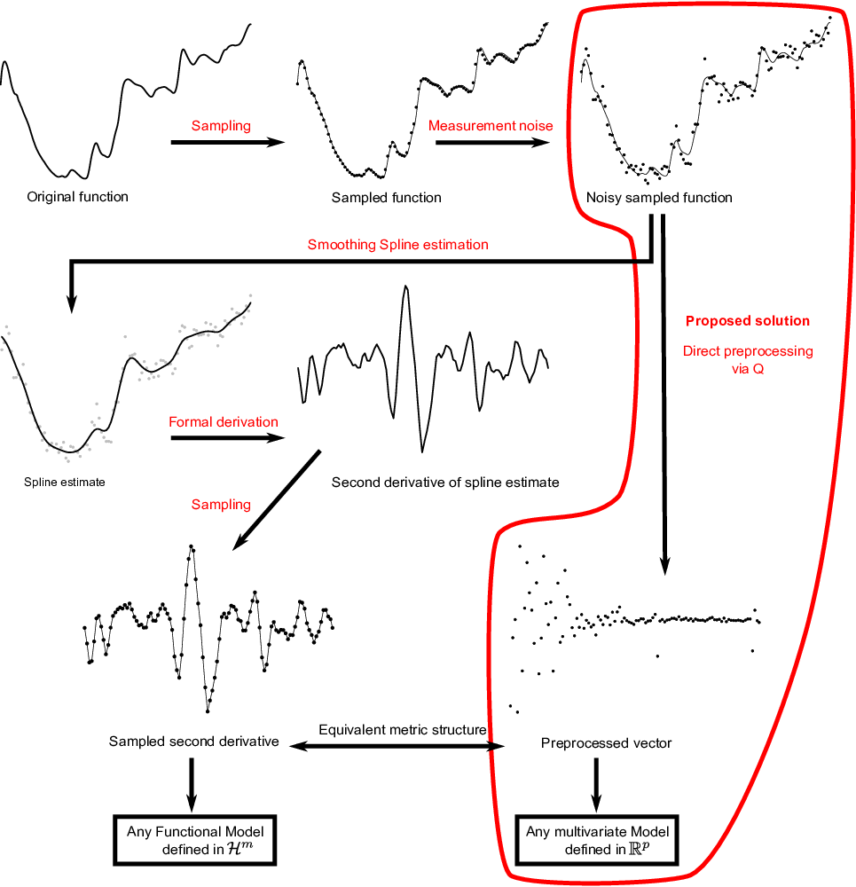
On a practical point of view, Wahba (1990) demonstrates that cross validated estimates of $\lambda$ achieve suitable convergence rates. Hence, steps 1 and 2 can be computed simultaneously by minimizing the total cross validated error for all the observations, given by

where $A$ is a $|\tau_{d}|\times|\tau_{d}|$ matrix called the influence matrix (see Wahba (1990)), over a finite number of $\lambda$ values.

Corollary 1 and Corollary 3 guarantee that the estimator proposed in the previous section is consistent:

While Theorem 3 is very general, it could be easily extended to cover special cases such as additional hypothesis needed by the estimation scheme or to provide data based parameter selections. We discuss briefly those issues in the present section.

It should first be noted that most estimation schemes, $\psi_{\mathcal{D}}$, depend on parameters that should fulfill some assumptions for the scheme to be consistent. For instance, in the Kernel Ridge Regression method in $\mathbb{R}^{p}$, with Gaussian kernel, $\psi_{\mathcal{D}}$ has the form given in Equation (7) where the $(\alpha_{i})$ are the solutions of

The method thus depends on the parameter of the Gaussian kernel, $\gamma$ and of the regularization parameter $\delta_{n}$. This method is known to be consistent if (see Theorem 9.1 of Steinwart and Christmann (2008)):

Additional conditions of this form can obviously be directly integrated in Theorem 3 to obtain consistency results specific to the corresponding algorithms.

Moreover, practitioners generally rely on data based selection of the parameters of the estimation scheme $\psi_{\mathcal{D}}$ via a validation method: for instance, rather than setting $\delta_{n}$ to e.g., $n^{-5}$ for $n$ observations (a choice which is compatible with theoretical constraints on $\delta_{n}$), one chooses the value of $\delta_{n}$ that optimizes an estimation of the performances of the regression function obtained on an independent data set (or via a re-sampling approach).

In addition to the parameters of the estimation scheme, functional data raise the question of the convenient order of the derivative, $m$, and of the sampling grid optimality. In practical applications, the number of available sampling points can be unnecessarily large (see Biau et al. (2005) for an example with more than 8 000 sampling points). The preprocessing performed by $\mathbf{Q}_{\lambda_{d},\tau_{d}}$ do not change the dimensionality of the data which means that overfitting can be observed in practice when the number of sampling points is large compared to the number of functions. Moreover, processing very high dimensional vectors is time consuming. It is there quite interesting in practice to use a down-sampled version of the original grid.

To select the parameters of $\psi_{D}$, the order of the derivative and/or the down-sampled grid, a validation strategy, based on splitting the dataset into training and validation sets, could be used. A simple adaptation of the idea of Berlinet et al. (2008); Biau et al. (2005); Laloë (2008); Rossi and Villa (2006) shows that a penalized validation method can be used to choose any combination of those parameters consistently. According to those papers, the condition for the consistency of the validation strategy would simply relate the shatter coefficients of the set of classifiers in $\mathbb{R}^{d}$ to the penalization parameter of the validation. Once again, this type of results is a rather direct extension of Theorem 3.

The methodology followed for the two illustrative datasets is roughly the same:

1. 1.

   the dataset is randomly split into a training set on which the model is estimated and a test set on which performances are computed. The split is repeated several times. The Tecator dataset (Section 6.2) is rather small (240 spectra) and exhibits a rather large variability in predictive performances between different random splits. We have therefore used 250 random splits. For the Yellow-berry dataset (Section 6.3), we used only 50 splits as the relative variability in performances is far less important.

2. 2.

   $\lambda$ is chosen by a global leave-one-out strategy on the spectra contained in training set (as suggested in Section 5.1). More precisely, a leave-one-out estimate of the reconstruction error of the spline approximation of each training spectrum is computed for a finite set of candidate values for $\lambda$. Then a common $\lambda$ is chosen by minimizing the average over the training spectra of the leave-one-out reconstruction errors. This choice is relevant as cross validation estimates of $\lambda$ are known to have favorable theoretical properties (see Craven and Wahba (1978); Utreras (1981) among others).

3. 3.

   for regression problems, a Kernel Ridge Regression (KRR) Saunders et al. (1998); Shawe-Taylor and Cristianini (2004) is then performed to estimate the regression function; this method is consistent when used with a Gaussian kernel under additional conditions on the parameters (see Theorem 9.1 of Steinwart and Christmann (2008)); as already explained, in the applications, Kernel Ridge Regression is performed both with a Gaussian kernel and with a linear kernel (in that last case, the model is essentially a ridge regression model). Parameters of the models (a regularization parameter, $\delta_{n}$, in all cases and a kernel parameter, $\gamma$ for Gaussian kernels) are chosen by a grid search that minimizes a validation based estimate of the performances of the model (on the training set). A leave-one-out solution has been chosen: in Kernel Ridge Regression, the leave-one-out estimate of the performances of the model is obtained as a by-product of the estimation process, without additional computation cost, see e.g. Cawley and Talbot (2004).
   Additionally, for a sake of comparison with a more traditional approach in FDA, Kernel Ridge Regression is compared with a nonparametric kernel estimate for the Tecator dataset (Section 6.2.1). Nonparametric kernel estimate is the first nonparametric approach introduced in Functional Data Analysis Ferraty and Vieu (2006) and can thus be seen as a basis for comparison in the context of regression with functional predictors. For this method, the same methodology as with Kernel Ridge Regression was used: the parameter of the model (i.e., the bandwidth) was selected on a grid search minimizing a cross-validation estimate of the performances of the model. In this case, a 4-fold cross validation estimate was used instead of a leave-one-out estimate to avoid a large computational cost.

4. 4.

   for the classification problem, a Support Vector Machine (SVM) is used Shawe-Taylor and Cristianini (2004). As KRR, SVM are consistent when used with a Gaussian kernel Steinwart (2002). We also use a SVM with a linear kernel as this is quite adapted for classification in high dimensional spaces associated to sampled function data. We also use a K-nearest neighbor model (KNN) for reference. Parameters of the models (a regularization parameter for both SVM, a kernel parameter, $\gamma$ for Gaussian kernels and number of neighbors K for KNN) are chosen by a grid search that minimizes a validation based estimate of the classification error: we use a 4-fold cross-validation to get this estimate.

5. 5.

   We evaluate the models obtained for each random split on the test set. We report the mean and the standard deviation of the performance index (classification error and mean squared error, respectively) and assess the significance of differences between the reported figures via paired Student tests (with level 1%).

6. 6.

   Finally, we compare models estimated on the raw spectra and on spectra transformed via the $\mathbf{Q}_{\lambda_{d},\tau_{d}}$ matrix for $m=1$ (first derivative) and $m=2$ (second derivative). For both values of $m$, we used the most classical boundary conditions ($x(0)=0$ and $Dx(0)=0$). Depending of the problem, other boundary conditions could be investigated but this is outside the scope of the present paper (see Besse and Ramsay (1986); Heckman and Ramsay (2000) for discussion on this subject). For the Tecator problem, we also compare these approaches with models estimated on first and second derivatives based on interpolating splines (i.e. with $\lambda=0$) and on first and second derivatives estimated by finite differences.
   Note that the kind of preprocessing used has almost no impact on the computation time. In general, selecting the parameters of the model with leave-one-out or cross-validation will use significantly more computing power than constructing the splines and calculating their derivatives. For instance, computing the optimal $\lambda$ with the approach described above takes less than 0.1 second for the Tecator dataset on a standard PC using our R implementation which is negligible compared to the several minutes used to select the optimal parameters of the models used on the prepocessed data.

The first studied dataset is the standard Tecator dataset Thodberg (1996) ¹¹ 1 Data are available on statlib at http://lib.stat.cmu.edu/datasets/tecator. It consists in spectrometric data from the food industry. Each of the 240 observations is the near infrared absorbance spectrum of a meat sample recorded on a Tecator Infratec Food and Feed Analyzer. Each spectrum is sampled at 100 wavelengths uniformly spaced in the range 850–1050 nm. The composition of each meat sample is determined by analytic chemistry and percentages of moisture, fat and protein are associated this way to each spectrum.

The Tecator dataset is a widely used benchmark in Functional Data Analysis, hence the motivation for its use for illustrative purposes. More precisely, in Section 6.2.1, we address the original regression problem by predicting the percentage of fat content from the spectra with various regression method and various estimates of the derivative preprocessing: this analysis shows that both the method and the use of derivative have a strong effect on the performances whereas the way the derivatives are estimated has almost no effect. Additionally, in Section 6.2.2, we apply a noise (with various variances) to the original spectra in order to study the influence of smoothing in the case of noisy predictors: this section shows the relevance of the use of a smoothing spline approach when the data are noisy. Finally, Section 6.2.3 deals with a classification problem derived from the original Tecator problem (in the same way as what was done in Ferraty and Vieu (2003)): conclusions of this section are similar to the ones of the regression study.

The goal of the last experiment is to predict the presence of yellow-berry in durum wheat (Triticum durum) kernels via a near infrared spectral analysis (see Figure 4). Yellow-berry is a defect of the durum wheat seeds that reduces the quality of the flour produced from affected wheat. The traditional way to assess the occurrence of yellow-berry is by visual analysis of a sample of the seed stock. In the current application, a quality measure related to the occurrence of yellow-berry is predicted from the spectrum of the seed.

The dataset consists in 953 spectra sampled at 1049 wavelengths uniformly spaced in the range 400–2498 nm. The dataset is split randomly into 600 learning spectra and 353 test spectra. Comparatively to the Tecator dataset, the variability of the results is smaller in the present case. We used therefore 50 random splits rather than 250 in the previous section.

The regression models were build via a Kernel Ridge Regression approach using a linear kernel and a Gaussian kernel. In both cases, the regularization parameter of the model is optimized by a leave-one-out approach. In addition, the width parameter of the Gaussian kernel is optimized via the same procedure at the same time.

The performance index is the mean squared error (M.S.E.). As a reference, the target variable has a variance of $0.508$. Results are summarized in Table 4 and Figure 5.

As in the previous section, we can rank the methods in increasing order of modelling error, we obtain the following result:

where G stands for Gaussian kernel and L for linear kernel (hence G-S2 stands for kernel ridge regression with gaussian kernel and smoothing splines with order 2 derivatives); $<$ corresponds to a significant difference (for a paired Student test with level 1%) and $\leq$ to a non significant one. For this application, there is a significant gain in using a non linear model (the Gaussian kernel). In addition, the use of derivatives leads to less contrasted performances that the ones obtained in the previous section but it still improves the quality of the non linear model in a significant way. In term of normalized mean squared error (mean squared error divided by the variance of the target variable), using a non linear model with the second derivatives of the spectra corresponds to an average gain of more than 5% (i.e., a reduction of the normalised mean squared error from 24% for the standard linear model to 18.6%).

In the original theorem (Lemma 3.1) in Kimeldorf and Wahba (1971), one has to verify that $(k_{0}(t_{l},.))_{l}$ spans $\mathcal{H}^{m}_{0}$ and that $(k_{1}(t_{l},.))_{l}$ are linearly independent. These are consequences of Assumption (A1).

First, $k_{0}(s,t)=\sum_{i,j=0}^{m-1}b_{ij}^{(-1)}s^{i}t^{j}$ where $\widetilde{B}=(b_{i,j}^{(-1)})_{i,j}$ is the inverse of $(\sum_{l=1}^{m}B^{l}s^{i}B^{l}t^{j})_{i,j}$ (see Heckman and Ramsay (2000)). Then $(k_{0}(t_{1},s),\ldots,k_{0}(t_{|\tau_{d}|},s))=(1,s,\ldots,s^{m-1})\widetilde{B}[V_{m-1}(t_{1},\ldots,t_{|\tau_{d}|})]^{T}$ where $V_{m-1}(t_{1},\ldots,t_{|\tau_{d}|})$ is the Vandermonde matrix with $m-1$ columns and $|\tau_{d}|$ rows associated to values $t_{1},\ldots,t_{|\tau_{d}|}$. If the $(t_{l})_{l}$ are distinct, this matrix is of full rank.

Moreover the reproducing property shows that $\sum_{l=1}^{|\tau_{d}|}a_{l}k_{1}(t_{l},.)\equiv 0$ implies $\sum_{l=1}^{|\tau_{d}|}a_{l}f(t_{l})\equiv 0$ for all $f\in\mathcal{H}^{m}_{1}$. Hence, $\mathcal{H}^{m}_{1}=\textrm{Ker}\left(B^{T},\sum_{l=1}^{\tau_{d}}a_{l}\zeta_{l}\right)^{T}$ where $\zeta_{l}$ denotes the linear form $h\in\mathcal{H}^{m}\rightarrow h(t_{l})$. As the co-dimension of $\mathcal{H}^{m}_{1}$ is $\textrm{dim}\mathcal{H}^{m}_{0}=m$ and as, by Assumption (A1), $B$ is linearly independent of $\sum_{l=1}^{\tau_{d}}a_{l}\zeta_{l}$, we thus have $\sum_{l=1}^{\tau_{d}}a_{l}\zeta_{l}\equiv 0$ (or $\textrm{codim}\,\textrm{Ker}\left(B^{T},\sum_{l=1}^{\tau_{d}}a_{l}\zeta_{l}\right)^{T}=\textrm{dim}\,\textrm{Im}\left(B^{T},\sum_{l=1}^{\tau_{d}}a_{l}\zeta_{l}\right)$ would be $m+1$). Thus, we obtain that $\sum_{l=1}^{|\tau_{d}|}a_{l}f(t_{l})\equiv 0$ for all $f$ in $\mathcal{H}^{m}$ and, as $(t_{l})$ are distinct, that $a_{l}=0$ for all $l$, leading to the independence conclusion for the $(k_{1}(t_{l},.))_{l}$.

References

- Bahlmann and Burkhardt (2004) Bahlmann, C., Burkhardt, H., 2004. The writer independent online handwriting recognition system frog on hand and cluster generative statistical dynamic time warping. IEEE Transactions on Pattern Analysis and Machine Intelligence 26, 299–310.
- Berlinet et al. (2008) Berlinet, A., Biau, G., Rouvière, L., 2008. Functional supervised classification with wavelets. Annales de l’ISUP 52, 61–80.
- Berlinet and Thomas-Agnan (2004) Berlinet, A., Thomas-Agnan, C., 2004. Reproducing Kernel Hilbert Spaces in Probability and Statistics. Kluwer Academic Publisher.
- Besse and Ramsay (1986) Besse, P., Ramsay, J., 1986. Principal component analysis of sampled curves. Psychometrika 51, 285–311.
- Biau et al. (2005) Biau, G., Bunea, F., Wegkamp, M., 2005. Functional classification in Hilbert spaces. IEEE Transactions on Information Theory 51, 2163–2172.
- Cardot et al. (1999) Cardot, H., Ferraty, F., Sarda, P., 1999. Functional linear model. Statistics and Probability Letters 45, 11–22.
- Cawley and Talbot (2004) Cawley, G., Talbot, N., 2004. Fast exact leave-one-out cross-validation of sparse least-squares support vector machines. Neural Networks 17, 1467–1475.
- Cox (1984) Cox, D., 1984. Multivariate smoothing splines functions. SIAM Journal on Numerical Analysis 21, 789–813.
- Craven and Wahba (1978) Craven, P., Wahba, G., 1978. Smoothing noisy data with spline functions. Numerische Mathematik 31, 377–403.
- Dauxois and Pousse (1976) Dauxois, J., Pousse, A., 1976. Les analyses factorielles en calcul des probabilités et en statistique : essai d’étude synthétique. Thèse d’État. Université Toulouse III.
- Dejean et al. (2007) Dejean, S., Martin, P., Baccini, A., Besse, P., 2007. Clustering time-series gene expression data using smoothing spline derivatives. EURASIP Journal on Bioinformatics and Systems Biology 2007, Article ID70561.
- Deville (1974) Deville, J., 1974. Méthodes statistiques et numériques de l’analyse harmonique. Annales de l’INSEE 15, 3–97.
- Devroye and Györfi (1985) Devroye, L., Györfi, L., 1985. Nonparametric Density Estimation: the view. John Wiley, New York.
- Devroye et al. (1994) Devroye, L., Györfi, L., Krzyżak, A., Lugosi, G., 1994. On the strong universal consistancy of nearest neighbor regression function estimates. The Annals of Statistics 22, 1371–1385.
- Devroye et al. (1996) Devroye, L., Györfi, L., Lugosi, G., 1996. A Probabilistic Theory for Pattern Recognition. Springer-Verlag, New York.
- Devroye and Krzyżak (1989) Devroye, L., Krzyżak, A., 1989. An equivalence theorem for convergence of the kernel regression estimate. Journal of Statistical Planning and Inference 23, 71–82.
- Faragó and Györfi (1975) Faragó, T., Györfi, L., 1975. On the continuity of the error distortion function for multiple-hypothesis decisions. IEEE Transactions on Information Theory 21, 458–460.
- Ferraty and Vieu (2003) Ferraty, F., Vieu, P., 2003. Curves discrimination: a non parametric approach. Computational and Statistical Data Analysis 44, 161–173.
- Ferraty and Vieu (2006) Ferraty, F., Vieu, P., 2006. NonParametric Functional Data Analysis. Springer.
- Ferré and Yao (2003) Ferré, L., Yao, A., 2003. Functional sliced inverse regression analysis. Statistics 37, 475–488.
- Györfi et al. (2002) Györfi, L., Kohler, M., Krzyżak, A., Walk, H., 2002. A Distribution-Free Theory of Nonparametric Regression. Springer, New York.
- Heckman and Ramsay (2000) Heckman, N., Ramsay, J., 2000. Penalized regression with model-based penalties. The Canadian Journal of Statistics 28, 241–258.
- James (2002) James, G., 2002. Generalized linear models with functional predictor variables. Journal of the Royal Statistical Society Series B 64, 411–432.
- James and Hastie (2001) James, G., Hastie, T., 2001. Functional linear discriminant analysis for irregularly sampled curves. Journal of the Royal Statistical Society, Series B 63, 533–550.
- James et al. (2000) James, G., Hastie, T., Sugar, C., 2000. Principal component models for sparse functional data. Biometrika 87, 587–602.
- James and Silverman (2005) James, G., Silverman, B., 2005. Functional adaptive model estimation. Journal of the American Statistical Association 100, 565–576.
- Kallenberg (1997) Kallenberg, O., 1997. Foundations of Modern Probability. Probability and its Applications, Spinger.
- Kimeldorf and Wahba (1971) Kimeldorf, G., Wahba, G., 1971. Some results on Tchebycheffian spline functions. Journal of Mathematical Analysis and Applications 33, 82–95.
- Laloë (2008) Laloë, T., 2008. A k-nearest neighbor approach for functional regression. Statistics and Probability Letters 78, 1189–1193.
- Lugosi and Zeger (1990) Lugosi, G., Zeger, K., 1990. Nonparametric estimation via empirical risk minimization. IEEE Transaction on Information Theory 41, 677–687.
- Mas and Pumo (2009) Mas, A., Pumo, B., 2009. Functional linear regression with derivatives. Journal of Nonparametric Statistics 21, 19–40. Submitted: under revision. Available at http://www.math.univ-montp2.fr/~mas/FLRD.pdf.
- Pollard (2002) Pollard, D., 2002. A User’s Guide to Measure Theoretic Probability. Cambridge University Press, Cambridge.
- Ragozin (1983) Ragozin, D., 1983. Error bounds for derivative estimation based on spline smoothing of exact or noisy data. Journal of Approximation Theory 37, 335–355.
- Ramsay and Dalzell (1991) Ramsay, J., Dalzell, C., 1991. Some tools for functional data analysis (with discussion). Journal of the Royal Statistical Society. Series B. Statistical Methodology 53, 539–572.
- Ramsay and Silverman (1997) Ramsay, J., Silverman, B., 1997. Functional Data Analysis. Springer Verlag, New York.
- Ramsay and Silverman (2002) Ramsay, J., Silverman, B., 2002. Applied Functional Data Analysis. Springer Verlag.
- Rossi and Conan-Guez (2005) Rossi, F., Conan-Guez, B., 2005. Functional multi-layer perceptron: a nonlinear tool for functional data anlysis. Neural Networks 18, 45–60.
- Rossi and Conan-Guez (2006) Rossi, F., Conan-Guez, B., 2006. Theoretical properties of projection based multilayer perceptrons with functional inputs. Neural Processing Letters 23, 55–70.
- Rossi et al. (2005) Rossi, F., Delannay, N., Conan-Guez, B., Verleysen, M., 2005. Representation of functional data in neural networks. Neurocomputing 64, 183–210.
- Rossi and Villa (2006) Rossi, F., Villa, N., 2006. Support vector machine for functional data classification. Neurocomputing 69, 730–742.
- Saunders et al. (1998) Saunders, G., Gammerman, A., Vovk, V., 1998. Ridge regression learning algorithm in dual variables, in: Proceedings of the Fifteenth International Conference on Machine Learning (ICML’98), Madison, Wisconsin, USA. pp. 515–521.
- Shawe-Taylor and Cristianini (2004) Shawe-Taylor, J., Cristianini, N., 2004. Kernel methods for pattern analysis. Cambridge University Press, Cambridge, UK.
- Steinwart (2002) Steinwart, I., 2002. Support vector machines are universally consistent. Journal of Complexity 18, 768–791.
- Steinwart and Christmann (2008) Steinwart, I., Christmann, A., 2008. Support Vector Machines. Information Science and Statistics, Springer.
- Thodberg (1996) Thodberg, H., 1996. A review of bayesian neural network with an application to near infrared spectroscopy. IEEE Transaction on Neural Networks 7, 56–72.
- Utreras (1981) Utreras, F., 1981. Optimal smoothing of noisy data using spline functions. SIAM Journal on Scientific Computing 2, 153–163.
- Utreras (1988) Utreras, F., 1988. Boundary effects on convergence rates for Tikhonov regularization. Journal of Approximation Theory 54, 235–249.
- Wahba (1990) Wahba, G., 1990. Spline Models for Observational Data. Society for Industrial and Applied Mathematics, Philadelphia, Pennsylvania.
- Williams et al. (2006) Williams, B., Toussaint, M., Storkey, A., 2006. Extracting motion primitives from natural handwriting data, in: In Proceedings of the International Conference on Artificial Neural Networks (ICANN).
- Zhao (1987) Zhao, L., 1987. Exponential bounds of mean error for the nearest neighbor estimates of regression functions. Journal of Multivariate Analysis 21, 168–178.