Optimal Decoding Algorithm for Asynchronous Physical-Layer Network CodingThanks: This work was partially supported by grants from the University Grants Committee of the Hong Kong Special Administrative Region, China (Project No. AoE/E-02/08; Project No. 2150537). This work was also supported by NSF of China (Project No. 60902016) and NSF of Guangdong (Project No. 10151806001000003).
Abstract
A key issue in physical-layer network coding (PNC) is how to deal with the asynchrony between signals transmitted by multiple transmitters. That is, symbols transmitted by different transmitters could arrive at the receiver with symbol misalignment as well as relative carrier-phase offset. In this paper, 1) we propose and investigate a general framework based on belief propagation (BP) that can effectively deal with symbol and phase asynchronies; 2) we show that for BPSK and QPSK modulations, our BP method can significantly reduce the SNR penalty due to asynchrony compared with prior methods; 3) we find that symbol misalignment makes the system performance less sensitive and more robust against carrier-phase offset. Observation 3) has the following practical implication. It is relatively easier to control symbol timing than carrier-phase offset. Our results indicate that if we could control the symbol offset in PNC, it would actually be advantageous to deliberately introduce symbol misalignment to desensitize the system to phase offset.
Index Terms:
physical-layer network coding, network coding, symbol synchronization, phase synchronizationI Introduction
Physical-layer network coding (PNC), first proposed in [1], is a subfield of network coding [2] that is attracting much attention recently. The simplest system in which PNC can be applied is the two-way relay channel (TWRC), where two end nodes exchange information with the help of a relay node in the middle, as illustrated in Fig. 1(a).
Compared with the conventional relay system, PNC doubles the throughput of TWRC by reducing the needed time slots from four to two. In PNC, in the first time slot, the two end nodes send signals simultaneously to the relay; in the second phase, the relay processes the superimposed signals and maps them to network-coded information for broadcast back to the end nodes. From the network-coded information, each end node then makes use of its self information to extract the information from the other end node.
A key issue in PNC is how to deal with the asynchrony between signals transmitted by multiple transmitters. That is, symbols transmitted by different transmitters could arrive at the receiver with symbol misalignment as well as relative carrier-phase offset.
Many previous works (e.g., [1, 3, 4]) found that symbol misalignment and carrier-phase offset will result in appreciable performance penalties. For BPSK modulation, [1] showed that the BER performance penalties due to the carrier phase asynchrony and symbol offset are both 3 dB in the worst case. For QPSK modulation, the penalty can be as large as 6 dB in the worst case when the carrier-phase offset is [4].
These earlier investigations led to a common understanding that near-perfect symbol and carrier-phase synchronization are important for good performance in PNC. We believe that this is a misconception, and that asynchronous PNC can have good performance if we use the right methods to deal with the asynchrony.
The study of BPSK PNC in [1, 3], for example, made use of suboptimal decoding methods at the relay for the asynchronous PNC case. Furthermore, the joint effect of symbol and phase asynchronies was not investigated. In this paper, we propose an optimal maximum-likelihood (ML) decoding method making use of a belief propagation (BP) algorithm that addresses symbol and phase asynchronies jointly. We find that the BER performance penalty can be reduced from 3 dB (using the method in [1, 3]) to less than 0.5 dB (using our method here) for the worst case.
In QPSK PNC, the penalty is larger than 6 dB [4] only when the symbols are perfectly aligned and when the phase offset is . We find that using our optimal BP decoding algorithm, when there is a 1/2 symbol misalignment, the penalty is less than 1 dB (compared with the case when symbol and phase are perfectly synchronized). Additionally, an interesting result is that with the 1/2 symbol misalignment, the spread of penalties under various carrier-phase offsets is no more than 0.5 dB. This means that symbol misalignment has the effect of desensitizing the performance of the system to carrier-phase offset. The practical implication is as follows:
In practice, it is easier to control symbol timing than carrier-phase offset because of the relative time scales involved. If we could control the symbol offset in PNC (e.g., [5] presented a method to synchronize symbols from different sources), it would actually be advantageous to deliberately introduce symbol misalignment so that the system is robust against uncontrollable phase offsets.
The remainder of this paper is organized as follows: Section II introduces the system model adopted by this paper. Section III classifies and defines synchronous PNC and asynchronous PNC. Section IV presents our BP ML decoding method for dealing with asynchrony in PNC. Numerical results are given in Section V. Finally, Section VI concludes this paper.
II System Model
We study the two-way relay channel as shown in Fig. 1, in which nodes A and B exchange information with the help of relay node R. We assume that all nodes are half-duplex, i.e., a node cannot receive and transmit simultaneously. We also assume that there is no direct link between nodes A and B.
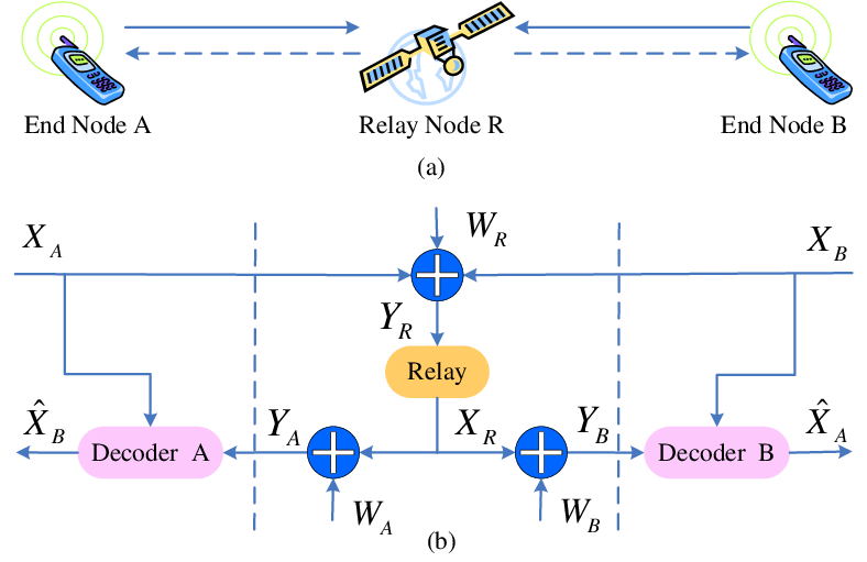
We consider a two-phase transmission scheme consisting of an uplink phase and a downlink phase. In the uplink phase, nodes A and B transmit packets to node R simultaneously. In the downlink phase, based on the overlapped signals received from A and B, R constructs a network-coded packet and broadcast the packet to A and B. Upon receiving the network-coded packet, A (B) then attempts to recover the original packet transmitted by B (A) in the uplink phase using self-information [1].
Consider the uplink phase again, if only A transmitted, then the received complex baseband signal at R (i.e., the received signal after down-conversion from the carrier frequency and low-pass filtering) would be
| (1) |
where is the received signal amplitude; are the symbols in the packet of A; is the pulse shaping function for the baseband signal; and is Gaussian noise with double-sided power spectral density for both the real and imaginary components within the baseband of interest. In the PNC set-up, A and B transmit simultaneously. In this case, the received complex baseband signal at R is
| (2) |
where ( is the relative phase offset between the signals from A and B due to phase asynchrony in their carrier-frequency oscillators, and difference in the delays of the two uplink channels); are the symbols in the packet of B; and is a time offset between the arrivals of the signals from A and B. Without loss of generality, we assume the signal of A arrives earlier than B. Furthermore, we assume is within one symbol period T. Thus, .11 1 If is more than one symbol period, we could generalize our treatment here so that is larger than the number of symbols in a packet. The packets will only be partially overlapping, with non-overlapping symbols at the front end and tail end. Essentially, our assumption of being within one symbol period implies that we are looking at the “worst case” with maximum overlapping between the two packets. When there are additional non-overlapping symbols at the front and tail ends, the decoding will have better error probability performance. We refer to and as the symbol and phase offsets (or misalignments) at R, respectively. Note that we have assumed a flat fading channel, and the channel gains stay constant within a packet duration. For simplicity, we assume power control so that . Furthermore, for convenience, we assume time is expressed in unit of symbol duration, so that . Then, we can rewrite (2) as
| (3) |
In general, the pulse shaping function can take different forms. To bring out the essence of our results in the simplest manner, throughout this paper, we assume the rectangular pulse shape: .
A critical design issue is how node R makes use of to construct a packet for broadcast to nodes A and B in the downlink phase. In this paper, we assume that R first oversamples to obtain signal samples. The signal samples will be used to construct an N-symbol packet for broadcast to A and B. The oversampling procedure is similar to that in [6] and described below. For
| (4) | ||||
| and | ||||
where , and (also ) and are a zero-mean complex Gaussian noise with variance and , respectively, for both the real and imaginary components.
Fig. 1(b) is a schematic diagram of our system. This paper adopts the following notation:
- •
denotes the source packet of node i, ;
- •
denotes the received packet (with the aforementioned oversampling) at relay node R;
- •
denotes the receiver noise at node R;
- •
denotes the network-coded packet at relay node R;
- •
denotes the received PNC packet at node i, ;
- •
denotes the receiver noise at node i, ;
- •
denotes the decoded source packet of node i, , at the other end node;
where is the number of source symbols. In the above, for BPSK, ; for QPSK, . In addition, .
III Synchronous vs. Asynchronous PNC
III-A Classification
Table I shows the four possible cases in PNC systems. Case 1 is the perfectly synchronized case studied in [1]; Case 2, in [3]; and Case 3, in [3, 8, 7]. This paper proposes a general scheme to tackle all four cases under one framework.
| (Case 1) | (Case 2) | |
| (Case 3) | (Case 4) |
III-B Review of Synchronous PNC (Case 1 in III-A)
Definition 1 (Synchronous PNC)
Synchronous PNC is the case where the two end nodes transmit their packets and in a synchronous manner so that the relay node R receives the combined signals with and . The received baseband packet at R is with N symbols. Node R then transforms into a network-coded packet for transmission in the downlink phase.
For this case, with reference to (4), since , the variance of the noise term is infinite, and the signal is contained only in the even terms . Thus, we can write
| (5) |
where , and is zero-mean Gaussian noise with variance for both the real and imaginary components.
For BPSK, . Only the real component of needs to be considered. For QPSK, since we are considering a synchronous system, the in-phase and quadrature-phase components in (5) are independent; it can therefore be considered as two parallel BPSK systems. In the following, we assume BPSK.
Let us consider a particular n, and omit the index n in our notation for simplicity. The a posteriori probability of the combination is given by
| (6) |
Let us use to represent bit 0 and to represent bit 1. Suppose that the downlink transmission also uses BPSK. For PNC output, , let us consider the XOR mapping: [1]. Then, if , and if . The following decision rule is used to map to :
| (7) |
III-C Asynchronous PNC (Case 2, 3 and 4 in III-A)
Definition 2 (Asynchronous PNC)
Asynchronous PNC is the case where the two end nodes transmit their packets and in an asynchronous manner so that the relay node R receives the combined signals with or . The received baseband packet at R is with symbols. Node R then transforms into a network-coded packet for transmission in the downlink phase.
The asynchronous case has been studied previously. However, suboptimal PNC mappings were considered. Refs. [1] and [3] argued that the largest BER performance penalty is 3 dB for BPSK modulation (for both phase and symbol asynchronies). These results, however, are based on suboptimal decoding methods. Ref. [4] mentioned that there is a maximum 6 dB BER performance penalty for QPSK modulation when and . To the best of our knowledge, no quantitative results and concrete explanation have been given for the QPSK case for general and .
Ref. [10] used an amplify-and-forward method in which the overlapped signals received at the relay are simply amplified and broadcasted back to the end nodes. This method does not require synchronization between the end nodes, but introduces some inefficiency, because the relay’s noise is forwarded along with the signal to the end nodes. Ref. [7] investigated systems in which symbols are aligned but phases are not. It uses QPSK for uplinks, but a higher order constellation map (e.g., 5QAM) for downlinks when the uplink phase offset is such that the use of QPSK will lead to poor performance. Ref. [11] investigated OFDM PNC. Because of the long duration of OFDM symbols in the frequency domain, the symbols from two end nodes can be considered as “almost aligned”. However, the phase offset is not addressed.
None of the prior methods attempt to look at the symbol and phase offset jointly. Furthermore, they try to “deal with” asynchrony, rather than to “exploit” asynchrony to gain performance advantage. As will be shown in this paper, we can exploit symbol asynchrony to gain robustness of the system against phase asynchrony.
IV A Belief Propagation PNC Decoding Scheme (BP-PNC)
This section presents a PNC decoding scheme based on belief propagation that deals with symbol and phase asynchronies jointly. We refer to the decoding method as BP-PNC. We make use of the oversampled symbols in (4) to construct a Tanner graph [9] as shown in Fig. 2. In the Tanner graph, denotes the evidence nodes, and there are such nodes; denotes the constraint nodes (also known as the compatibility or check nodes); and X denotes the source (or variable) nodes. We aim to decode the combination in . For simplicity, we use to denote . Note that the Tanner graph has a tree structure. This means that BP can find the exact solution for the a posteriori probability at each source node. Furthermore, the solution can be found after only one iteration of the message-passing algorithm (see [9]). From the decoded , we can then find the maximum a posteriori probability (MAP) XOR value, . In summary, BP can converge quickly and is MAP-optimal as far as the BER of is concerned. Note that the MAP optimal scheme is also ML optimal because each of the possible symbol values for and are equally likely (i.e., , where , and is the alphabet of modulated symbols.).
IV-1 BP-PNC Design
Let us now consider QPSK modulation, in particular, we define as the symbol set. With reference to (4), we have and , where . Define . Note that here, is computed based on only, and not on the whole . Also, is fixed and does not change throughout the message passing algorithm in the Tanner graph. and for are given as follows:
| (8) |
| (9) |
Note that except for the first and last symbols, each of and has 16 possible combinations (4 possibilities for and 4 possibilities for ). The first and last symbols have 4 possibilities, as follows: and
IV-2 Message Update Rules

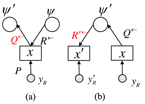
Given the evidence node values computed by (8) and (9), we now derive the message update rules for BP-PNC. Since the Tanner graph (in Fig. 2) for BP-PNC has a tree structure, the decoding of the joint probability can be done by passing the messages only once on each direction of an edge [12]. As described below, we could consider the right-bound messages first followed by the left-bound messages.
We represent messages on the edges with respect to the compatibility nodes in Fig. 2 by and . Specifically, () is the message connected to the right (left) of the k-th compatibility node. is a probability vector, where each component is the joint conditional probability of given of a particular combination. Similarly, and are also probability vectors, where and are probabilities and , respectively, for the right-bound messages as shown in the Step 1 (note here, for the left-bound message and are probabilities and correspondingly).
We omit the index k to avoid cluttering in the following discussion of message-update rules. We follow the principles and assumptions of the BP algorithm to derive the update equations, i.e., the output of a node should be consistent with the inputs while adopting a ‘sum of product’ format of the possible input combinations [12].
Step 1. Update of right-bound messages
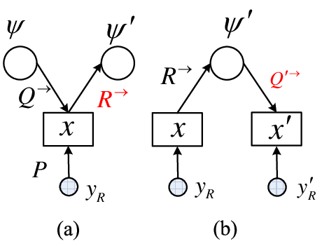


With reference to Fig. 4(a), we derive the update equations for the right-bound message based on the right-bound message and the fixed message from the evidence node . Based on the sum-product principle of the BP algorithm, we have
| (10) |
For the input message into the leftmost compatibility node, however, we should modify (10) with .
With reference to Fig. 4(b) we derive the update equations for the message based on the input message of the compatibility node. Note that for and , the common symbol overlapping in two adjacent samples is , thus we have
| (11) |
where and is a normalization factor to ensure that the sum of probabilities . If and , then the common symbol is . We have
| (12) |
where and is a normalization factor to ensure that the sum of probabilities .
We then update the next evidence node message based on the newly updated in Fig. 4(b) and in Fig. 4(a), and so on and so forth, until we reach rightmost node.
Step 2. Update of left-bound messages
With reference to Fig. 4(a) and (b), we use a similar procedure as in Step 1 to update the left-bound messages.
After steps 1 and 2 above, the values of the messages converge, thanks to the tree structure of the Tanner graph. We then compute the 4-tuple.
where . The maximum-likelihood is given by the that yields the largest element among the four elements. Note that we only use , and not , to obtain , because the information required to get is fully captured in .
V Numerical Results
This section presents simulation results for BP-PNC. We compare the performance of asynchronous PNC with that of the perfectly synchronized case [1], focusing on BPSK and QPSK modulations. For comparison purposes, the transmit amplitude per symbol in the QPSK case is made to be of that in the BPSK case so that they have the same energy per bit. In particular, is the energy per bit in the Fig. 6. The ideal synchronous QPSK curve therefore overlaps with the synchronous BPSK curve (because when symbols and phase are synchronized in QPSK, the system can be considered as two parallel BPSK systems).
V-A Summary of results
Our simulations yield the following findings:
- •
- •
For QPSK, the BER performance penalty due to phase asynchrony can be as high as 6-7 dB when the symbols are aligned, as can be seen from Fig. 6(a). However, with half symbol misalignment, our BP decoding algorithm can reduce the penalty to less than 1 dB, thanks to a “diversity and certainty propagation” effect (to be explained).
- •
Symbol misalignment makes the system more robust against phase asynchrony under our ML decoding method.
V-B Detailed description
Fig. 6 and Fig. 6 show the simulation results for BPSK and QPSK modulations, respectively. The x-axis is the average per-bit SNR of both end nodes, and the y-axis is the average .
For each data point, we simulate 10,000 packets of 2,048 bits. We use the synchronous PNC as a benchmark to evaluate BP-PNC. As can be seen from Fig. 6(a) and (b), the BER performance penalties due to phase and symbol asynchronies are less than 0.5 dB for all SNR regimes for BPSK. That is, for BPSK, BP-PNC reduces the BER performance penalty from 3dB in [1] to only 0.5 dB. Note that BP-PNC uses complex sampling that samples the 2-D information in the In-phase and Quadrature-phase components of the signal, whereas the scheme in [1] only samples in one dimension. For optimality, complex sampling is required in BPSK PNC because of the phase offset.
For QPSK with symbol synchrony but phase asynchrony, as can be seen from Fig. 6(a), the BER performance penalty can be as large as 6 to 7 dB. However, with half symbol misalignment, as can be seen from Fig. 6(b), BP-PNC reduces the penalty to within 1 dB (compared with the benchmark case where symbol and phase are perfectly synchronized). In other words, symbol asynchrony can ameliorate the penalty due to phase asynchrony. This can be explained by the “diversity and certainty propagation” effects elaborated in the next subsection. In addition, we note from Fig. 6(b) that when there is a half symbol offset, the phase offset effect becomes much less significant. Specifically, the spread of SNRs for a fixed BER under different phase offsets is less than 0.5 dB.
V-C Diversity and Certainty Propagation
In QPSK, each symbol has four possible values. Thus, the joint symbol from both sources has 16 possible values. The constellation map of the joint symbol varies according to the phase offset. Fig. 8 shows the constellation map of a joint symbol when the phase offset is , where the 16 diamonds corresponding to the 16 possibilities. For example, a point with value corresponds to the joint symbol in Fig. 7 due to the phase shift (i.e., ). In PNC, the 16 possibilities need to be mapped to four XOR possibilities for the PNC symbol. In Fig. 7, the diamonds are grouped into groups of four different colors. The diamonds of the same color are to be mapped to the same XOR PNC symbol according to . In this mapping process, some of the constellation points are more prone to errors than other constellation points, and the BER is dominated by these bad constellation points.

With reference to Fig. 7, the eight diamonds within the green circle are “bad constellation points”. Adjacent points among the 8 points are mapped to different XOR values, but the distances among two adjacent points are short. By contrast, the eight points outside the green circle are “good constellation points” because the distances among adjacent points are large. When symbols are synchronized (i.e., ), there are altogether joint symbols. On average, half of them will be bad constellation points with high BER.
Now, consider what if there is symbol asynchrony, say . We have joint symbols, out of which about will be good constellation points. A symbol from a source is combined with two symbols from the other sources to form two joint symbols received at the relay. Both the joint symbols have to be bad for poor performance. Thus, the diversity itself may give some improvement. In addition, there is a certainty propagation effect, as explained below.
Consider a good constellation point, say . For this point, we may be able to decode not just the XOR, but the individual values of and with high certainty. Now, suppose that the next joint symbol is a bad constellation point. But since we have good certainty about from the previous good constellation point, the uncertainly in can be reduced by the certainty propagated from with the BP algorithm. In other words, once is known, is not a bad constellation point anymore. Certainty can propagate along successive symbols from left to right, as well as from right to left, as shown in Fig. 8. Certainty propagation significantly reduces BER.

VI Conclusion and Future Work
This paper has proposed and investigated an optimal maximum likelihood (ML) decoding algorithm based on belief propagation, called BP-PNC, for asynchronous PNC. This method significantly improves the BER performance of the prior methods when there are symbol and phase asynchronies in the PNC system. In addition, we find that with symbol misalignment, BP-PNC desensitizes the BER performance to carrier-phase offset. In practice, it is relatively easier to control symbol timing than carrier-phase offset because of the relative time scales involved. Our results suggest that if we could control the symbol offset in PNC (e.g., using the method in [5]), it would actually be advantageous to deliberately introduce symbol misalignment so that the system is robust against uncontrollable phase offsets.
Prior to this work, it has often been thought that strict synchronization is needed for PNC. Our work, however, suggests that the penalty due to asynchrony can be nullified to a large extent with the BP-PNC decoding method. Our work is based on BPSK and QPSK modulations. We believe the same conclusion can be drawn for other modulations, particularly those with dense constellations. In addition, channel coding (with or without symbol offset in the system) also has the diversity and certainly propagation effects of symbol offset expounded in Section V-B. Thus, we believe that the incorporation of channel coding will also lessen the negative effect of asynchrony in PNC systems. These conjectures remain to be investigated in future work.
References
- [1] S. Zhang, S. C. Liew, and P. P. Lam. “Hot topic: physical layer network coding,” in Proc. 12th MobiCom, pp. 358-365, NY, USA, 2006.
- [2] R. Ahlswede, N. Cai, S.-Y. R. Li, and R. W. Yeung, “Network information flow,” IEEE Trans. on Information Theory, vol. 46, pp. 1204-1216, 2000.
- [3] S. Zhang, S. C. Liew, and P. P. Lam, “On the Synchronization of Physical-Layer Network Coding,” Information Theory Workshop, Oct 2006.
- [4] Y. Hao, D. Goeckel, Z. Ding, D. Towsley, and K. K. Leung, “Achievable rates for network coding on the exchange channel,” in Proc. of IEEE MILCOM, Orlando, Fla, USA, October 2007.
- [5] H. Rahul, H. Hassanieh, and D. Katabi, “SourceSync: A Cooperative Wireless Architecture for Exploiting Sender Diversity,” accepted by ACM SIGCOMM, 2010.
- [6] L. Lu, S. C. Liew, and S. Zhang, “Channel-coded Collision Resolution by Exploiting Symbol Misalignment,” in Proc. IEEE ICC 2010.
- [7] T. Koike-Akino, P. Popovski, and V. Tarokh, “Optimized constellations for two-way wireless relaying with physical network coding,” IEEE J. on Selected Areas in Comm., vol. 27, no. 5, pp. 773-787, June 2009.
- [8] S. Zhang, S. C. Liew, and L. Lu, “Physical Layer Network Coding Schemes over Finite and Infinite Fields,” in Proc. IEEE GLOBECOM 2008.
- [9] F. R. Kschischang, B. J. Frey, and H.-A. Loeliger, “Factor graphs and the sum-product algorithm,” IEEE Trans. on Inform. Theory, vol. 47, no. 2, Feb. 2001.
- [10] S. Katti, S. Gollakota, and D. Katabi, “Embracing Wireless Interference: Analog Network Coding,” ACM SIGCOMM, 2007.
- [11] Rossetto, F. and Zorzi, M., “On the design of practical asynchronous physical layer network coding,” IEEE 10th Workshop on SPAWC, 2009
- [12] J.S. Yedidia, W.T. Freeman, and Y. Weiss, “Understanding belief propagation and its generalizations,” Technical Report TR2001-22, MERL, 2001.