The chiral crossover, static-light and light-light meson spectra, and the deconfinement crossover
Abstract:
We study the chiral crossover, the spectra of light-light and of static-light mesons and the deconfinement crossover at finite temperature T. Our framework is the confining and chiral invariant quark model, related to truncated Coulomb gauge QCD. Since we are dealing with light quarks, where the linear potential dominates the quark condensate and the spectrum, we only specialize in the linear confining potential for the quark-antiquark interaction. We utilize T dependent string tensions previously fitted from lattice QCD data, and a fit of previously computed dynamically generated constituent quark masses. We scan the T effects on the constituent quark mass, on the meson spectra and on the polyakov loop.
January 24-28, 2011
Bormio, Italy
1 Introduction

Our main motivation is to contribute to understand the QCD phase diagram [1], for finite and . The QCD phase diagram is scheduled to be studied at LHC, RHIC and FAIR, and is sketched in Fig 1. Notice that, after enormous theoretical efforts, the analytic crossover nature of the finite-temperature QCD transition was finally determined by Y. Aoki et al. [2], utilizing Lattice QCD and physical quark, and reaching the continuum extrapolation with a finite volume analysis.
Here we utilize the Coulomb gauge hamiltonian formalism of QCD, presently the only continuum model of QCD able to microscopically include both a quark-antiquark confining potential and a vacuum condensate of quark-antiquark pairs. This model is able to address excited hadrons as in Fig. 2, and chiral symmetry at the same token, and we recently suggested that the infrared enhancement of the quark mass can be observed in the excited baryon spectrum at CBELSA and at JLAB [3, 4]. Thus the present work, not only addresses the QCD phase diagram, but it also constitutes the first step to allow us in the future to extend the computation of nay hadron spectrum, say the Fig. 2 computed in reference [3], to finite .

Both for the study of the hadron spectra, and for the study the QCD phase diagram, a finite quark mass is relevant. In the phase diagram, a finite current quark mass affects the position of the critical point between the crossover at low chemical potential and the phase transition at higher . Moreover the current quark mass affects the QCD vacuum energy density , relevant for the dark energy of cosmology. This all occurs in the dynamical generation of the quark mass . While the quark condensate is a frequently used order parameter for chiral symmetry breaking, the mass gap, i. e. the quark mass at vanishing momentum is another possible order parameter for chiral symmetry breaking.

Here we address the finite temperature string tension, the quark mass gap for a finite current quark mass and temperature, and the deconfinement and chiral restoration crossovers. We conclude on the separation of the critical point for chiral symmetry restoration from the critical point for deconfinement.

2 Fits for the finite T string tension from the Lattice QCD energy
At vanishing temperature , the confinement, due to the formation of chromo-electric and chromo-magnetic flux tubes as shown in Figs. 3 and 4, can be modelled by a string tension, dominant at moderate distances,
| (1) |
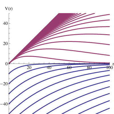
At short distances we have the Luscher or Nambu-Gotto Coulomb potential due to the string vibration plus the One Gluon Exchange Coulomb potential, however the Coulomb potential is not important for chiral symmetry breaking. At finite temperature the string tension should also dominate chiral symmetry breaking, and thus one of our crucial steps here is the fit of the string tension obtained from the Lattice QCD data for the quark-antiquark free energy of the Bielefeld Lattice QCD group, [5, 6, 7, 8, 9].
At finite temperature, the quark, or the quark-antiquark free energies, can be computed utilizing Polyakov loops, as in Fig. 5. The Polyakov loop is a gluonic path, closed in the imaginary time (proportional to the inverse temperature ) direction in a periodic boundary Euclidian Lattice discretization of QCD. They measures the free energy of one or more static quarks,
| (2) |
If we consider a single solitary quark in the universe, in the confining phase, his string will travel as far as needed to connect the quark to an antiquark, resulting in an infinite energy F. Thus the 1 quark Polyakov loop is a frequently used order parameter for deconfinement. With the string tension extracted from the pair of Polyakov loops we can also estimate the 1 quark Polyakov loop .
At finite , we use as thermodynamic potentials the free energy , computed in Lattice QCD with the Polyakov loops [5, 6, 7, 8, 9], and illustrated in Fig. 6. It is related to the static potential with adequate for isothermic transformations. In Fig. 7 we extract the string tensions from the free energy computed by the Bielefeld group, and we also include string tensions previously computed by the Bielefeld group [10].
We also find an ansatz for the string tension curve, among the order parameter curves of other physical systems related to confinement, i. e. in ferromagnetic materials, in the Ising model, in superconductors either in the BCS model or in the Ginzburg-Landau model, or in string models, to suggest ansatze for the string tension curve. We find that the order parameter curve that best fits our string tension curve is the spontaneous magnetization of a ferromagnet [11], solution of the algebraic equation,
| (3) |
In Fig. 8 we show the solution of Eq. 3 obtained with the fixed point expansion, and compare it with the string tensions computed from lattice QCD data.

3 The mass gap equation with finite and finite current quark mass .
Now, the critical point occurs when the phase transition changes to a crossover, and the crossover in QCD is produced by the finite current quark mass m0, since it affects the order parameters or , and the mass gap or the quark condensate . Moreover utilizing as order parameter the mass gap, i. e. the quark mass at vanishing moment, a finite quark mass transforms the chiral symmetry breaking from a phase transition into a crossover. For the study of the QCD phase diagram it thus is relevant to determine how the current quark mass affects chiral symmetry breaking, in particular we study in detail the effect of the finite current quark mass on chiral symmetry breaking, in the framework of truncated Coulomb gauge QCD with a linear confining quark-antiquark potential.


The most fundamental information for the quark-antiquark interaction in QCD comes from the Wilson loop in Lattice QCD, providing the confining quark-antiquark potential for a static quark-antiquark pair. This potential is consistent with the funnel potential, also utilized in the quark model to describe the quark-antiquark sector of meson spectrum, in particular to describe the linear behaviour of mesonic Regge trajectories. Notice that the short range Coulomb potential could also be included in the interaction, but here we ignore it since it only affects the quark mass through ultraviolet renormalization [12], which is assumed to be already included in the current quark mass. Here we specialize in computing different aspects of chiral symmetry breaking with linear confinement . Since we are interested in working at finite temperature we utilize a recent fit of lattice QCQ data with a temperature dependent string tension .

To address the light quark sector it is not sufficient to know the static quark-antiquark potential, we also need to know what Dirac vertex to use in the quark-antiquark-interaction. This vertex is necessary to study not only the meson spectrum but also the dynamical spontaneous breaking of chiral symmetry. To determine what vertex to use, we review how the quark-antiquark potential can be approximately derived from QCD, in two different gauges. In Coulomb gauge [13],
| (4) |
the interaction potential, as derived by Szczepaniak and Swanson [14, 15], is a density-density interaction, with Dirac structure . Another approximate path from QCD considers the modified coordinate gauge of Balitsky [16] and in the interaction potential for the quark sector, retains the first cumulant order, of two gluons [17, 18, 19]. This again results in a simple density-density effective confining interaction. As in QCD, this only has one scale, say , in the interaction, since both the quark condensate and the hadron spectrum turn out to be insensitive to any constant in the potential. Thus our framework is similar to an expansion of the QCD interaction, truncated to the leading density-density term, where the confining quark-antiquark potential is a linear potential.


While this is not exactly equivalent to QCD, our framework maintains three interesting aspects of non-pertubative QCD, a chiral invariant quark-antiquark interaction, the cancellation of infrared divergences [20, 21, 22, 23, 24, 25], and a quark-antiquark linear potential [26, 27, 28, 14, 29, 30]. Importantly, since our model is well defined and solvable, it can be used as a simpler model than QCD, and yet qualitatively correct, to address different aspects of hadronic physics. In particular here we study how chiral symmetry breaking occurs at finite temperature and chemical potential , in the realistic case of small but finite current quark masses. Thus we apply our framework to the phase diagram of QCD.
Our interaction potential for the quark sector is,
| (5) | |||||
where the density-density interaction includes just the linear confining potential together with an infrared constant, which may be possibly divergent.
The mass gap equation and the energy of a quark are determined from the Schwinger-Dyson equation at one loop order using the Hamiltonian of Eq. (5). for a recent derivation with all details see [31]. The interaction in the four momentum of the potential and quark propagator term includes an integral in the energy
| (6) |
which factorizes trivially from the vector momentum integral. Using spherical coordinates, the angular integrals can be performed analytically and finally only an integral in the modulus of the momentum remains to be computed numerically. We arrive at the mass gap equation in two equivalent forms, of a non-linear integral functional equation,
| (7) | |||||
and of a minimum equation of the energy density ,
| (8) | |||
where the functions and are angular integrals of the Fourier transform of the potential. In what concerns the one quark energy we get,
| (9) | |||||


In the chiral limit of massless current quarks, the breaking of chiral symmetry is spontaneous. But for a finite current quark mass, some dynamical symmetry breaking continues to add to the explicit breaking caused by the quark mass. The mass gap equation at the ladder/rainbow truncation of Coulomb Gauge QCD in equal time reads,
| (10) | |||
The mass gap equation (10) for the running mass is a non-linear integral equation with a nasty cancellation of Infrared divergences [32, 33, 34]. We devise a new method with a rational ansatz, and with relaxation [31], to get a maximum precision in the IR where the equation extremely large cancellations occur. Since the current quark masses of the six standard flavours span over five orders of magnitude from 1.5 MeV to 171 GeV, we develop an accurate numerical method to study the running quark mass gap and the quark vacuum energy density from very small to very large current quark masses. The solution is shown in Fig. 10 for a vanishing momentum .
At finite , one only has to change the string tension to the finite T string tension of Eq. (3), for different quark masses [35], and also to replace an integral in by a discrete sum in Matsubara Frequencies. Both are equivalent to a reduction in the string tension, and thus all we have to do is to solve the mass gap equation in units of . The results are depicted in Fig. 10. Thus at vanishing we have a chiral symmetry phase transition, and at finite we have a crossover, that gets weaker and weaker when increases. This is also sketched in Fig. 10.
4 Infrared regularization of the linear confining potential and the Matsubara sum
Notice that in the case of a linear potential, divergent in the infrared, the Fourier transform needs an infrared regulator eventually vanishing. We illustrate two possible infrared regularizations of the linear potential if Fig. 9.
A possible regularization of the linear potential is,
| (11) |
corresponding to a model of confinement where the quark-antiquark system has an infinite binding energy at the origin , is monotonous and only vanishes at an arbitrarily large distance. This potential has a simple three-dimensional Fourier transform,
| (12) | |||||
and this is the most common form of the linear potential in momentum space utilized in the literature. Notice that this is infrared divergent due to the infinite binding energy in the limit where the regulator .

If we want to avoid the infinite binding energy we should use a different regularization of the linear potential, also vanishing when but not monotonous since it grows linearly at the origin starting with ,
| (13) |
where the Fourier transform,
| (14) |
is such that the integrals in no longer diverge. For instance,
| (15) |
since this is proportional to . The new term in the potential is equal to in the limit , and this potential is infrared finite. Both the potentials in Eqs. (11) and (13) are illustrated in Fig. 9.
In the vanishing temperature limit the different regularizations lead to the same physical results since any constant term in a density-density interaction has no effect in the quark running mass or in the hadron spectrum [31]. The regularizations only contribute to the potential and the one-quark energy, but it occurs that these contributions exactly cancel in the chiral order parameters, and in the hadron spectrum.

However at the two different regularizations may lead to different physical results.
In the mass gap equation or Schwinger Dyson equation, we have the Minkowski space integral in of the quark propagator pole of Eq. (6) and this is equivalent to an integral in in Euclidian space after a Wick rotation in the Argand space,
| (16) |
real axis the path corresponds to and in the imaginary axis the path corresponds to .
Notice that the integral in Eq. (16) is only identical to the one in Eq. (6) if the one quark energy . If the integral of Eq. (16) changes sign, and this is consistent with the pole moving from the fourth quadrant to the third quadrant of the Argand plane. While the integral in Eq. (6) is insensitive to this translation of the pole, the Wick rotation leads to a pole correction. For simplicity, we choose to work with positive one quark energies only .
In finite temperature and density , the continuous euclidian space integration of eq. (16) is extended to the sum in Matsubara frequencies,
| (17) |
It is clear that in the vanishing temperature and density limit one gets back the initial Euclidean space integral of eq. (16), when the Matsubara sum approaches the continuum integration with .

Notice that at the results depend on the constant in the potential. Since the Matsubara sum depends on the one quark energy , and a constant shift of the potential added to the linear term, say , affects the energy by a , thus weakening the finite effects scaling like . On the other hand if the shift is small enough to produce at some a negative energy , at vanishing density , then the Matsubara sum could break down.
Thus we study here only one scenario for the constant potential shift , present anyway in the different possible infrared regularizations of the linear potential. Our scenario consists in a maximum energy, with as in the standard regularization of the linear potential of Eq. (11). In that case and the Matsubara sum is simply constant, producing always the result of . Our results are shown in Figs. 11 and 12.
We don’t explore this second possible scenario here, leaving it for a future study, consisting in having the minimal , closer to the regularization of the linear potential of Eq. (13), just sufficient to cancel the one quark energy at vanishing momentum . In that case the Matsubara sum makes a larger difference, interpolating between at vanishing momentum and at large momentum. But we expect that, whatever the contribution of the Matsubara sum is, the temperature dependence of the string tension is the dominant finite effect, and thus for a first exploration our first scenario is sufficient.
5 Chiral symmetry and confinement crossovers with a finite current quark mass
We now study whether the two main phase transitions in the QCD phase diagram, confinement and chiral symmetry breaking, have two different two critical points or a coincident one. Confinement drives chiral symmetry breaking, and at small density both transitions are a crossover, and not a first or second order phase transition due to the finite quark mass.
However the quark mass affects differently these two phase transitions in the QCD. In what concerns confinement, the linear confining quark-antiquark potential saturates when the string breaks at the threshold for the creation of a quark-antiquark pair. Thus the free energy of a single static quark is not infinite, it is the energy of the string saturation. The saturation energy is of the order of the mass of a meson i. e. of . For the Polyakov loop we get,
| (18) |
Thus at infinite we have a confining phase transition, while at finite we have a crossover, that gets weaker and weaker when decreases. This is sketched in Figs. 13 and 14.

Since the finite current quark mass affects in opposite ways the crossover for confinement and the one for chiral symmetry, we conjecture that at finite and there are not only one but two critical points (a point where a crossover separates from a phase transition). Since for the light and quarks the current mass is small, we expect the crossover for chiral symmetry restoration critical to be closer to the vertical axis, and the crossover for deconfinement to go deeper into the finite region of the critical curve in the QCD phase diagram depicted in Fig. 1.
We now compute the hadron spectrum, in particular the meson spectra. In what concerns the light meson masses are dominated by the linear confining potential. At , the string tension vanishes, the confining potential disappears, and thus all light hadrons decrease their mass until they melt at . Notice that chiral symmetry is not entirely restored because increases with . Nevertheless, with , the masses and wavefunctions do essentially scale with , and thus also essentially vanish at . This is sketched in Fig. 15. A comparable vanishing of light meson masses also occurs in the sigma model [36].
6 Outlook
We remark that the pure gauge string tension is well fitted by the condensed matter physics magnetization curve , and we utilize it.
We compute the dynamically generated quark mass , solving the mass gap equation both for finite current quark masses and for finite . The finite current quark masses turn both the confinement and the chiral symmetry phase transitions into two different crossovers.
We qualitatively study the full spectra of light hadrons at finite , including the excited spectra, and conclude that the light hadron masses essentially vanish at . The light hadrons all melt at , since the masses and wavefunctions essentially scale with .
We soon plan to complete the part of this work which is only sketched here, i. e. to compute the excited hadron spectrum at finite , continuing the work initiated with Tim Van Cauteren, Marco Cardoso, Nuno Cardoso and Felipe Llanes-Estrada [3], and to compute and compare the crossover curves for the chiral symmetry restoration and for the deconfinement at finite .
References
- [1] CBM Progress Report, publicly available at http://www.gsi.de/fair/experiments/CBM, (2009).
- [2] Y. Aoki, G. Endrodi, Z. Fodor, S. D. Katz and K. K. Szabo, Nature 443, 675 (2006) [arXiv:hep-lat/0611014].
- [3] P. Bicudo, M. Cardoso, T. Van Cauteren and F. J. Llanes-Estrada, Phys. Rev. Lett. 103, 092003 (2009) [arXiv:0902.3613 [hep-ph]].
- [4] P. Bicudo, Phys. Rev. D 81, 014011 (2010) [arXiv:0904.0030 [hep-ph]].
- [5] M. Doring, K. Hubner, O. Kaczmarek and F. Karsch, Phys. Rev. D 75, 054504 (2007) [arXiv:hep-lat/0702009].
- [6] K. Hubner, F. Karsch, O. Kaczmarek and O. Vogt, arXiv:0710.5147 [hep-lat].
- [7] O. Kaczmarek and F. Zantow, Phys. Rev. D 71, 114510 (2005) [arXiv:hep-lat/0503017].
- [8] O. Kaczmarek and F. Zantow, arXiv:hep-lat/0506019.
- [9] O. Kaczmarek and F. Zantow, PoS LAT2005, 192 (2006) [arXiv:hep-lat/0510094].
- [10] O. Kaczmarek, F. Karsch, E. Laermann and M. Lutgemeier, Phys. Rev. D 62, 034021 (2000) [arXiv:hep-lat/9908010].
- [11] R. Feynamn, R. Leighton, M. Sands, ”The Feynman Lectures on Physics”, Vol II, chap. 36 ”Ferromagnetism”, published by Addison Wesley Publishing Company, Reading, Massachussets, ISBN 0-201-02117-x (1964).
- [12] P. Bicudo, Phys. Rev. D 79, 094030 (2009) [arXiv:0811.0407 [hep-ph]].
- [13] T.D. Lee, Particle Physics and Introduction to Field Theory, (Harwood Academic Pub- lishers, New York, 1981).
- [14] A. Szczepaniak, E. S. Swanson, C. R. Ji and S. R. Cotanch, Phys. Rev. Lett. 76, 2011 (1996) [arXiv:hep-ph/9511422].
- [15] A. P. Szczepaniak and E. S. Swanson, Phys. Rev. D 55, 1578 (1997) [arXiv:hep-ph/9609525].
- [16] I. I. Balitsky, Nucl. Phys. B 254, 166 (1985).
- [17] H. G. Dosch, Phys. Lett. B 190, 177 (1987).
- [18] H. G. Dosch and Yu. A. Simonov, Phys. Lett. B 205, 339 (1988).
- [19] P. Bicudo, N. Brambilla, E. Ribeiro and A. Vairo, Phys. Lett. B 442, 349 (1998) [arXiv:hep-ph/9807460].
- [20] A. Le Yaouanc, L. Oliver, O. Pene, J. C. Raynal, Phys. Lett. 134B, 249 (1984).
- [21] A. Amer, A. Le Yaouanc, L. Oliver, O. Pene and J.-C. Raynal, Phys. Rev. Lett. 50, 87 (1983).
- [22] A. Le Yaouanc, L. Oliver, O. Pene and J.-C. Raynal, Phys. Rev. D 29, 1233 (1984);
- [23] A. Le Yaouanc, L. Oliver, S. Ono, O. Pène and J. C. Raynal, Phys. Rev. D 31, 137 (1985).
- [24] Y. L. Kalinovsky, L. Kaschluhn and V. N. Pervushin, Phys. Lett. B 231, 288 (1989).
- [25] P. Bicudo, J. E. Ribeiro, Phys. Rev. D 42, 1611 (1990); Phys. Rev. D 42, 1625 (1990); Phys. Rev. D 42, 1635 (1990).
- [26] S. L. Adler, A. C. Davis, Nucl. Phys. B 244, 469 (1984),
- [27] P. Bicudo, J. E. Ribeiro and J. Rodrigues, Phys. Rev. C 52, 2144 (1995).
- [28] R. Horvat, D. Kekez, D. Palle and D. Klabucar, Z. Phys. C 68, 303 (1995).
- [29] F. J. Llanes-Estrada, S. R. Cotanch, Phys. Rev. Lett. 84, 1102 (2000).
- [30] R. F. Wagenbrunn and L. Y. Glozman, Phys. Rev. D 75, 036007 (2007) [arXiv:hep-ph/0701039].
- [31] P. Bicudo, arXiv:1007.2044 [hep-ph].
- [32] S. L. Adler and A. C. Davis, Nucl. Phys. B 244, 469 (1984).
- [33] P. J. A. Bicudo and A. V. Nefediev, Phys. Rev. D 68, 065021 (2003) [arXiv:hep-ph/0307302].
- [34] F. J. Llanes-Estrada and S. R. Cotanch, Phys. Rev. Lett. 84, 1102 (2000) [arXiv:hep-ph/9906359].
- [35] P. Bicudo, Phys. Rev. D82, 034507 (2010). [arXiv:1003.0936 [hep-lat]].
- [36] E. Seel, S. Strüber, F. Giacosa, D. H. Rischke ”Chiral symmetry restoration in linear and nonlinear O(N) models within the auxiliary field method,” invited talk at Excited QCD 2011, Les Houches, France, February 2011.
- [37] P. Bicudo, M. Cardoso, P. Santos, J. Seixas, [arXiv:0804.4225 [hep-ph]].
- [38] P. Bicudo, J. Seixas, M. Cardoso, [arXiv:0906.2676 [hep-ph]].