Tail-induced spin-orbit effect in the gravitational radiation of compact binaries
Abstract
Gravitational waves contain tail effects which are due to the back-scattering of linear waves in the curved space-time geometry around the source. In this paper we improve the knowledge and accuracy of the two-body inspiraling post-Newtonian (PN) dynamics and gravitational-wave signal by computing the spin-orbit terms induced by tail effects. Notably, we derive those terms at 3PN order in the gravitational-wave energy flux, and 2.5PN and 3PN orders in the wave polarizations. This is then used to derive the spin-orbit tail effects in the phasing through 3PN order. Our results can be employed to carry out more accurate comparisons with numerical-relativity simulations and to improve the accuracy of analytical templates aimed at describing the whole process of inspiral, merger and ringdown.
pacs
04.30.-w, 04.25.-gI Introduction
I.1 Motivation
During the last ten years a network of ground-based laser-interferometer gravitational-wave detectors has been built and has taken data at design sensitivity. It is a worldwide network composed of the Laser Interferometer Gravitational wave Observatory (LIGO), Virgo, GEO-600, and TAMA and it has operated in the frequency range Hz. Coalescing binary systems composed of black holes and/or neutron stars are among the most promising sources for those detectors. By the gravitational-wave detectors will be upgraded to a sensitivity such that event rates for coalescing binary systems will increase by approximately a factor one thousand, thus making likely the first detection of gravitational waves from those systems. In the future, space-based detectors like LISA should detect supermassive black-hole binary systems in the low frequency band Hz.
The search for gravitational waves from coalescing binary systems and the extraction of source parameters are based on the matched-filtering technique, which requires a rather accurate knowledge of the waveform of the incoming signal. In particular, the detection and subsequent data analysis are made by using a bank of templates modeling the gravitational wave emitted by the source. The need of a faithful template bank has driven the development of accurate templates over the last thirty years.
The post-Newtonian (PN) expansion is the most powerful approximation scheme in analytical relativity capable of describing the two-body dynamics and gravitational-wave emission of inspiraling compact binary systems [1]. The PN expansion is an expansion in the ratio of the characteristic orbital velocity of the binary to the speed of light . However, as the black holes approach each other toward merger, we expect the PN expansion to lose accuracy because the velocity of the holes approaches the speed of light. At that point, numerical relativity (NR) [2, 3, 4] plays a crucial role providing us with the dynamics and gravitational-wave emission of the last cycles of inspiral, followed by the merger and ringdown phases. Furthermore, by properly combining PN predictions and NR results, it is possible to describe analytically and/or numerically with high accuracy, the full gravitational-wave signal [6, 7, 8, 5].
Black holes in binary systems can carry spin, and when spins are not aligned with the orbital angular momentum, spins induce precession of the orbital plane (see e.g. Ref. [9]). This adds substantial complexity to the gravitational waveforms, making it indispensable to include spin effects in templates used for the search. Moreover, as found long time ago [10, 11, 12, 13, 14, 15, 16, 18, 17], gravitational waves contain tail effects which are due to the back-scattering of linear waves in the curved space-time geometry around the source (and primarily generated by its mass). This causes the gravitational-wave signal to depend on the entire history of the binary system.
In this paper we improve the knowledge and accuracy of the two-body inspiraling dynamics and gravitational-wave signal by computing the spin-orbit (SO) terms induced by tail effects. This is the continuation of our previous work on spins [19, 20] where we obtained the next-to-leading 2.5PN SO contributions in the equations of motion and gravitational-wave energy flux. Here, we derive those SO terms at 3PN order in the gravitational-wave energy flux, where they are entirely due to tails. Furthermore we obtain the SO terms at 2.5PN and 3PN orders in the wave polarizations that are specifically due to tails, leaving aside other SO terms at these orders that come from instantaneous (non-tail) linear contributions and which will not be computed here.
We obtain the energy flux in two independent ways, first directly using the radiative multipole moments, and second by differentiating and squaring the gravitational-wave polarizations. To compute the SO tail effects in the wave polarizations we solve the two-body dynamics taking into account spin precession. Assuming quasi-circular adiabatic inspiral, we also compute the 3PN SO terms induced by tails in the gravitational-wave phasing. These results can be used to improve the accuracy of inspiraling templates, to carry out comparison with numerical-relativity predictions, and to improve the accuracy of effective-one-body and phenomenological templates [6, 7, 8, 5].
As an important check of our results we obtain the 3PN SO tail terms in the energy flux in the test-particle limit, and find perfect agreement with earlier PN computations based on black-hole perturbation induced by the motion of a test particle around a massive black hole [21].
This paper is organized as follows. In Sec. II we review the post-Newtonian multipole moment formalism and discuss relevant properties of tails. In Sec. III, we describe how spin effects are included in the PN formalism and derive the binary’s evolution equations when black holes carry spins. In Sec. IV we obtain the time evolution of the moving triad and solve the precessing dynamics at the relevant PN order. In Sec. V we compute the 2.5PN and 3PN SO tail effects in the gravitational waveform and polarizations. Restricting ourselves to quasi-circular adiabatic inspiral, we derive in Sec. VI the 3PN SO tail effects in the energy flux and in the gravitational phasing. Section VII contains our main conclusions. In Appendix A we check that the equations of motion do not contain physical SO effects at 3PN order. In Appendix B we investigate the secular evolution of the spins, and finally in Appendix C we give the explicit gravitational-wave polarizations.
I.2 Notation
In this paper we adopt the following notations. is the Newton constant and is the speed of light. As usual we refer to PN as the post-Newtonian terms with formal order relative to the Newtonian acceleration in the equations of motion, or to the lowest-order quadrupole-moment formalism for the radiation field. Greek indices are space-time indices, and Latin are space indices. The quantity denotes a multi-index composed of multipolar spatial indices ranging from 1 to 3. Similarly and ; is the product of spatial vectors (similarly for ). We indicate with and the product of partial derivatives . In the case of summed-up (dummy) multi-indices , we do not write the summations from 1 to 3 over their indices. Furthermore, the symmetric-trace-free (STF) projection is indicated using brackets, ; thus and for STF moments. For instance we write . The transverse-traceless (TT) projection operator is denoted where is the projector orthogonal to the unit direction of a radiative coordinate system . The quantity is the Levi-Civita antisymmetric symbol such that . Finally, we denote time derivatives with a superscript , and we indicate the symmetrization operation with round parentheses.
II Wave generation formalism
The gravitational waveform , generated by an isolated source described by a stress-energy tensor with compact support, and propagating in the asymptotic regions of the source, is the TT projection of the metric deviation at the leading-order in the distance to the source. It is parametrized by STF mass-type moments and current-type ones , which constitute the observables of the waveform at infinity from the source and are called the radiative moments [22]. The general expression of the TT waveform, in a suitable radiative coordinate system , reads, when neglecting terms of the order of or higher,
| (1) |
Here the radiative moments and are functions of the retarded time in the radiative coordinate system (we denote ). The integer refers to the multipolar order, and is the unit vector pointing from the source to the far away detector. The TT projection operator and other notations are defined in Sec. I.2. With and denoting two unit polarization vectors, orthogonal and transverse to the direction of propagation , the two “plus” and “cross” polarization states of the waveform read as
| (2a) | ||||
| (2b) | ||||
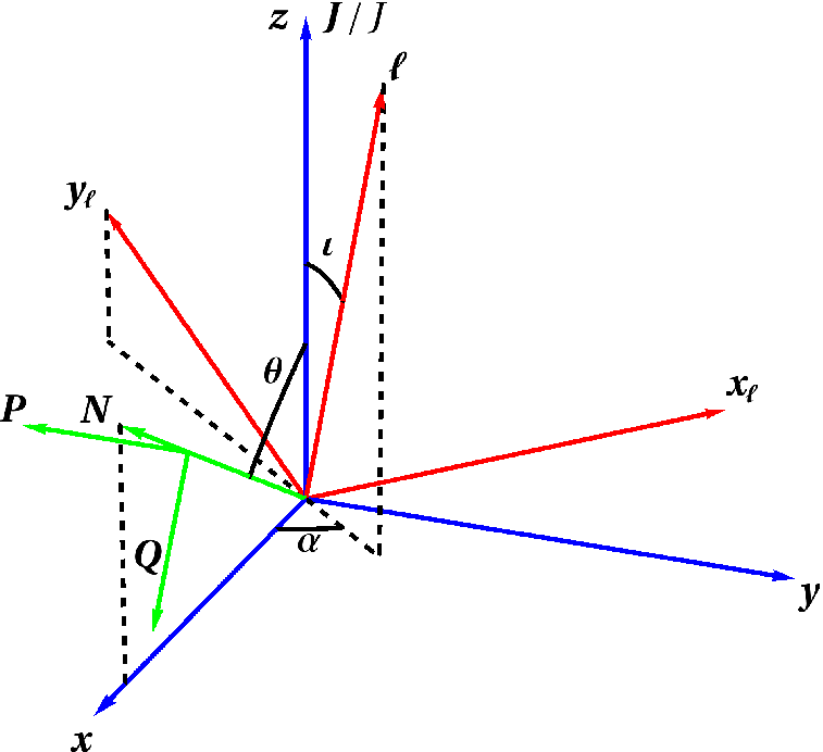
Our convention for the choice of the polarization vectors and in the case of binary systems will be specified in Fig. 2. Plugging Eq. (1) into the standard expression for the gravitational-wave energy flux we get [22]
| (3) |
II.1 Expression of the radiative moments
In the multipolar-post-Minkowskian formalism [13, 14, 15], the radiative moments are expressed in terms of two other sets of moments, referred to as the “canonical” moments , , and which are relevant to the description of the source’s near zone. The relation between the radiative moments , and the canonical ones , encodes all the non-linearities in the wave propagation between the source and the detector [15]. Those relations may be re-expanded in a PN way and are then seen to contain, at the leading 1.5PN order, the contribution of the so-called gravitational-wave tails, due to backscattering of linear waves onto the space-time curvature associated with the total mass of the source itself. The explicit expressions at 1.5PN order are [15, 23]
| (4a) | ||||
| (4b) | ||||
where is the Arnowitt-Deser-Misner (ADM) mass associated with the source. It also coincides with the mass monopole moment. The remainders in Eqs. (4) denote some correction terms which are at least of order 1.5PN and are instantaneous or contain the non-linear memory effect which will not be considered in the present computation. Here and denote some numerical constants given by [23]
| (5a) | ||||
| (5b) | ||||
The constant in Eqs. (4) is a freely specifiable time scale entering the relation between the radiative time and the corresponding retarded time in harmonic coordinates.
The canonical moments and are themselves linked to six sets of multipole moments characterizing the source, collectively called the “source” moments and denoted , , , , , . The point is that those source moments are known as explicit integrals extending over the pseudo-energy-momentum tensor of the matter fields and the gravitational field of the source [23, 24]. In the following we shall essentially need and which represent the main mass and current moments of the source. The other moments , , and play a little role because they are associated with a possible gauge transformation performed at linear order. It turns out that the difference between the canonical moments , and the source moments , arises only at the 2.5PN order:
| (6a) | |||
| (6b) | |||
For the present application it will be sufficient to consider the source mass moments at 1PN order and the current ones at Newtonian order (see the discussion in Sec. III.2). These are given by [25]
| (7a) | ||||
| (7b) | ||||
The other moments we shall need are the mass monopole moment and the monopole of the moment , which are given by
| (8a) | ||||
| (8b) | ||||
The mass, current and tensor densities , , in Eqs. (7)–(8), are defined as (where )
| (9) |
We recall that, e.g., in Eqs. (7) means taking -time derivatives.
The spin parts of the source moments in Eqs. (7) will come from the model we adopt for the stress-energy tensor appropriate to spinning compact binaries (see details in Sec. III). Importantly, we notice that for the accuracy required by our calculation of the spin effects due to tails all integrands in Eqs. (7) have compact support. This is in contrast with the spin effects at 2.5PN order which necessitate non-compact supported higher-order terms in the source moments [20]. (We also find that the second term in can be ignored in the present application to spins.)
II.2 Computing the tail integrals
The tail integrals in Eqs. (4) extend over the entire past of the evolving source and it is a priori a non trivial task to compute them. Here we recall, based on Refs. [15, 16], that the tails are actually very weakly sensitive (in a post-Newtonian sense) to the past history of the source, and can essentially be computed using the current dynamics, i.e. at current time , of the source.
We have to compute, e.g., the integral appearing in the radiative mass multipole moment (4a), in which we can replace, following (6a), the canonical moment by the source moment . Thus,
| (10) |
where we pose .
Let us introduce a constant time interval to split the integral (10) into some contribution coming from the “recent past”, and extending from the current time to , and the remaining contribution called the “remote past”, from to in the past. The recent past can be thought of as corresponding to the most recent orbital period of a compact binary system, while the remote past will include the details (eventually unknown) of the formation and early past evolution of the compact binary. However we shall prove that our result is independent of the chosen time scale .
To control the convergence of the tail integral (10) in the past we make a physical assumption regarding the behavior of the multipole moment when . We assume that at very early times the source was formed from a bunch of freely falling particles initially moving on some hyperbolic-like orbits, and forming at a later time a gravitationally bound system by emission of gravitational radiation. The gravitational motion of initially free particles is given by , where and denote constant vectors, and (see Ref. [26] for a proof; to simplify we consider the relative motion of two particles with total mass ). Here the Landau remainder -symbol satisfies . From that physical assumption we find that the multipole moment behaves when like
| (11) |
where , and are constant tensors. The time derivatives of the moment appearing in Eq. (10) are therefore dominantly like
| (12) |
which ensures that the integral (10) is convergent.
Next we integrate the “remote-past” integral (from to ) by parts and make use of our assumption (11)–(12) to arrive at (posing )
| (13) | |||||
At this stage it is convenient to perform a Fourier decomposition of the multipole moment, i.e.
| (14) |
(The Fourier coefficients satisfy since the moment is real.) Inserting (14) into (13) we obtain a closed-form result in the Fourier domain thanks to the mathematical formula [27]
| (15) |
where , with and denoting the sign and the absolute value, and being the Euler constant. Finally the result reads
| (16) |
We observe that the arbitrary time scale has cancelled from this result.
Later we shall apply this result to the computation of the waveform and energy flux of a spinning compact binary system. A priori, since the tail integral (10) depends on all the past history of the binary (with the current binary’s dynamics being the result of its long evolution by gravitational radiation emission), we expect that the binary’s continuous spectrum of frequencies should contain all orbital frequencies at any epoch in the past, say with , besides the current orbital frequency . However, it has been shown in the Appendix of Ref. [16] that one can actually compute the tail integral by considering only the current frequency . Indeed the error made by this procedure is small in a post-Newtonian sense, being of the order of , where denotes the adiabatic parameter associated with the gravitational radiation emission, and evaluated at the current time . In a PN expansion we have so the error made by replacing the past dynamics by the current one is of the order of and can be neglected. The proof given in Ref. [16] is based on a simple model of binary evolution in the past, where an always circular orbit is decaying by radiation following the lowest order quadrupole formula, and spins are neglected. In this paper we shall assume that this result remains valid for spinning binaries.
III Applications to spinning binaries
III.1 Spin vectors for point-like objects
Following our previous work [19, 20] we base our calculations on the model of point-particles with spins [28, 29, 30, 31, 32, 33, 34, 35, 36, 37, 38, 39, 40]. The stress-energy tensor of a system of spinning particles is the sum of a monopolar piece, made of Dirac delta-functions, plus the dipolar or spin piece, made of gradients of delta-functions:
| (17) |
where is the four-dimensional Dirac function, is the field point, is the world-line of particle , is the four-velocity, such that where denotes the metric at the particle’s location, is the linear momentum of the particle, and denotes its antisymmetric spin angular momentum. Our notation and conventions are the same as in Refs. [19, 20] which provide more details, except that here we shall denote using an overbar (i.e. ) the original spin variable used in [19, 20]. Note that with our convention the spin variable has the dimension of an angular momentum times .
In order to fix unphysical degrees of freedom associated with an arbitrariness in the definition of in the case of point particles (and associated with the freedom in the choice for the location of the center-of-mass worldline of extended bodies), we adopt the covariant supplementary spin condition also called Tulczyjew condition [33, 34]:
| (18) |
which allows the natural definition of the spin four-vector in such a way that
| (19) |
where is the four-dimensional antisymmetric Levi-Civita symbol (such that ). For the spin vector itself, we choose a four-vector that is purely spatial in the particle’s instantaneous rest frame, which means that in any frame
| (20) |
This choice is also adopted in Refs. [41, 42, 43, 44]. As a consequence of the condition (18), we can check that the mass defined by is constant along the trajectories, i.e. .
Important simplifications occur in the case of SO interactions, which are linear in the spins. Neglecting quadratic (spin-spin) interactions, the linear momentum is simply linked to the four velocity as , so the supplementary spin condition (18) reduces to , and the equation of evolution of the spins is given by
| (21) |
which means that the spin is parallely transported along the particle’s trajectory.
Following [19, 20] we adopt in a first stage as the vector spin variable the contravariant components of the vector , which are obtained by raising the index on by means of the spatial metric , denoting the inverse of the covariant spatial metric evaluated at point (i.e. such that ). Hence our initial spin variable is
| (22) |
This definition of the spin vector agrees with the choice already made in Refs. [43, 44].
At the leading SO approximation, the contravariant spin variables defined by Eq. (22) coincide with the spin variables with constant magnitude broadly used in the literature (see, e.g., Ref. [42]). At the next-to-leading order, the variables differ from constant magnitude spins and their relationship has been worked out at 2PN order in Eq. (7.4) of Ref. [20]. In the present paper we shall denote the constant magnitude spins by (although they were denoted in Refs. [19, 20]). We know that it is actually better when presenting final results to switch to the constant magnitude spins since they have a simpler precession equation (and turn out to be secularly conserved, i.e., over a radiation-reaction time scale; see Ref. [45] and Appendix B below).
For two bodies () the relationship between the constant magnitude spins and the original spin variables up to 1PN order is:
| (23) |
together with the relation for the other particle obtained by exchanging all particle labels. We denote by the coordinate velocity of the particle (with mass ) and by the relative distance. See Ref. [20] for more accurate formulas extending (23) to 2PN order. In the present paper we shall consistently work only with the constant magnitude spins .
In the case of binary systems it is convenient to pose
| (24a) | ||||
| (24b) | ||||
where and (with ). In addition we find it useful to occasionally use the dimensionless spin variables
| (25) |
III.2 Multipole moments with spin-orbit effects
The matter-source densities (9) depend on the components of the stress-energy tensor. At the leading PN order, the spin contribution therein (indicated by the subscript S) reduce to
| (26a) | ||||
| (26b) | ||||
| (26c) | ||||
where means the three-dimensional Dirac delta-function evaluated on the particle 1, and means the same quantity but corresponding to the particle 2.
In Ref. [20] the SO terms have been computed in the source mass quadrupole moment up to next-to-leading 2.5PN order and the source current quadrupole moment up to next-to-leading 1.5PN order. All the other source moments were computed at the leading SO order. Those results are sufficient for our purpose. Actually, to compute the specific contributions of tails we need only the moments at leading SO order, given for general by
| (27a) | ||||
| (27b) | ||||
Because the leading SO terms scale as in the mass source moments, and as in the current source moments, the number of non-linear terms needed in the radiative moments [Eqs. (60) below] is small. We refer to Sec. V of [20] for higher-order expressions of SO contributions of the source quadrupole moments.
III.3 Equations of motion with spin-orbit effects
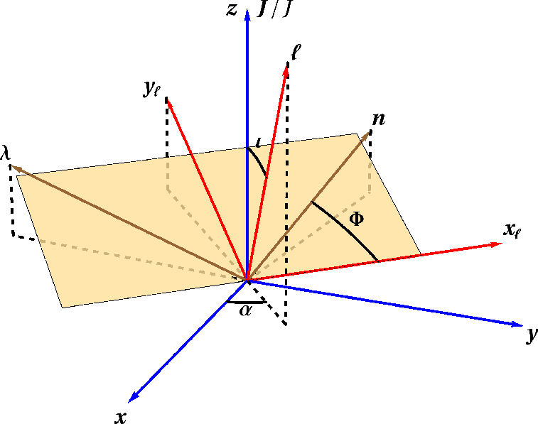
Here we investigate the case where the binary’s orbit is nearly circular, i.e., whose radius is constant apart from small perturbations induced by the spins (as usual we neglect the gravitational radiation damping at 2.5PN order). We denote by the relative position of the particles (and ). Following Ref. [42] we introduce an orthonormal moving triad defined by as before, where with denotes the Newtonian orbital angular momentum and the symmetric mass ratio, and . Those vectors are represented on Fig. 1, which shows the geometry of the system. The orbital frequency is defined for general, not necessarily circular orbits, by where represents the derivative of with respect to the coordinate time . It is also equal to the scalar product of and which we denote as . The components of the acceleration along the basis are then given by
| (28a) | ||||
| (28b) | ||||
| (28c) | ||||
We project out the spins on this orthonormal basis, defining and similarly for . Next we impose the restriction to quasi-circular precessing orbits which is defined by the conditions so that (neglecting radiation reaction damping terms). In this way we find [19] that the equations of the relative motion in the frame of the center-of-mass are
| (29) |
There is no component of the acceleration along . Comparing with Eqs. (28) in the case of circular orbits, we see that is indeed the orbital frequency, while what we call the “precessional frequency” is proportional to the variation of in the direction of the velocity . We know that is given by
| (30) |
where we denote and , where the spin variables are defined by Eq. (25). The PN parameter is and we have included only the 1PN non-spin term and the leading SO correction at 1.5PN order. On the other hand, we get [19]
| (31) |
where . At the leading 1.5PN SO order the orbital frequency (30), as well as , remain unchanged if we were to substitute some other variables to the spins , . However, when working at a higher PN approximation, it is more convenient to use the spin variables , , built from the constant magnitude spins. The main advantage of the spins is that they satisfy the usual-looking precession equations
| (32) |
showing that the spins precess around the direction of , and at the rate . The equation (32) could in principle be extended to any PN order (at the linear SO level). The precession’s angular-frequency vectors have been computed up to the 2PN order for circular orbits in Ref. [20]. Here, we shall only need the 1PN leading order:
| (33) |
To obtain we simply have to change into . Both precession frequencies are constant in magnitude and independent of the spins in the 1.5PN dynamics.
The equations of motion (29) and the precession equations (32) together leave invariant the total angular momentum,
| (34) |
where denotes the orbital angular momentum. For future reference we give the components of along the triad basis at 1PN order for non-spin effects and at the leading 1.5PN order for spin ones [19, 20]:
| (35a) | ||||
| (35b) | ||||
| (35c) | ||||
Note that the components and are due to spin effects arising at order . See Eq. (7.10) of Ref. [20].
IV Evolution of the triad
Using Eq. (29) the time derivatives of the three moving triad vectors can be expressed with respect to that triad basis as
| (36a) | ||||
| (36b) | ||||
| (36c) | ||||
Equivalently, introducing the orbital precession vector and spin precession vector , these equations can be written as
| (37a) | ||||
| (37b) | ||||
| (37c) | ||||
We recall that the spin precession frequency is given by Eq. (31) or equivalently
| (38) |
where we pose which defines a gauge-invariant PN parameter agreeing with at leading order.
We shall now solve the evolution equations for the moving triad at the 1.5PN order in the conservative dynamics (i.e., neglecting radiation reaction). We recall that the spin variables we use in this calculation are those with constant magnitude, denoted here .
It is convenient to introduce a fixed (inertial) orthonormal basis ; see Figs. 1 and 2. For a given value of the total angular momentum (a constant vector), and of the direction of the detector as seen from the source, a canonical choice of the basis vectors is as follows: (i) is defined to be the normalized value of , namely ; (ii) is orthogonal to the plane spanned by and and points to the direction that corresponds to the positive orientation of the acute angle , i.e. ; (iii) completes the triad. We see that , and are coplanar by construction. Then, we introduce the standard spherical coordinates with the inclination angle measured from the zenith direction and the azimuthal angle measured from . The spherical coordinates of and are denoted as and respectively, and since lies in the same plane as and , we have (see Fig. 2). Since is the angle between the total and orbital angular momenta, we have
| (39) |
The angles are referred to as the precession angles.
We now derive the time evolution of our triad vectors from that of the precession angles , and of an appropriate phase that specifies the position of with respect to some reference direction. Following Ref. [46], we introduce the unit vectors
| (40) |
such that is an orthonormal basis. The phase angle is defined by (see Fig. 1):
| (41) |
The rotation takes place in the instantaneous orbital plane spanned by and , and we have
| (42a) | ||||
| (42b) | ||||
from which we deduce
| (43) |
Combining (43) with (39) we also get
| (44) |
By identifying the right-hand sides of Eqs. (36) or (37) with the time-derivatives of the identities (42) we obtain the following system of equations for the variations of , and , equivalent to the system (36),
| (45a) | ||||
| (45b) | ||||
| (45c) | ||||
On the other hand, using the total angular momentum (34) together with the components of the orbital angular momentum given by Eqs. (35) — notably the fact that and are due to SO terms dominantly of order , we deduce that is a small quantity of order . From this fact, we conclude by direct integration of the sum of Eq. (45a) and Eq. (45c) that
| (46) |
in which we have defined the “carrier” phase as
| (47) |
with the value of the carrier phase at some arbitrary initial time . We recall that the orbital frequency (30) is constant in first approximation for circular motion.
The combination being known by Eq. (46), we can further express the precession angles and in first approximation in terms of the components and of the total spin . From (39) we find (discarding non-linear spin contributions)
| (48) |
where we recall that denotes the Newtonian orbital angular momentum. On the other hand, using also Eq. (44) and the relation (46) we obtain at leading order
| (49) |
It remains now to obtain the explicit time variation of the components of the individual spins , and . Using (48) and (49) [and also (46)] we shall then be able to obtain the explicit time variation of the precession angles and phase. Combining (32) and (36) we obtain the precession equations for the three unknowns , and in the form of the following first-order system (valid at any PN approximation)
| (50a) | ||||
| (50b) | ||||
| (50c) | ||||
where is the norm of the precession vector of the spin as given by (33), and the precession frequency is explicitly given by (38). Actually the terms involving in the right-hand sides of (50) can be neglected because they are quadratic in the spins. Thus, staying at the linear SO level, we find that the equations (50) can be decoupled and integrated as
| (51a) | ||||
| (51b) | ||||
| (51c) | ||||
Here and denote two constants for each spins , and agree with the projections (which are constant at the linear SO level) of the spins perpendicular and parallel to the direction of the orbital angular momentum . The phase of each of the spins is given by
| (52) |
where is the constant initial phase at time .
With those results we obtain an explicit solution for the precession angles by substituting Eqs. (51) into the results (48) and (49). We find that is given at the 0.5PN level by
| (53) |
where we recall that . Knowing we deduce from
| (54) |
The difference of spin phases readily follows from Eq. (52) and Eq. (33) at 1PN order as
| (55) |
Moreover, Eq. (44) can be written more explicitly at the 1.5PN level as
| (56) |
where is given at the 1.5PN order by
| (57) | ||||
and the 1PN orbital angular momentum is known from Eq. (35a).
As a check of the previous solution we observe that if we take the time derivative of Eq. (39), then evaluate the total angular momentum given by (34) together with the components of the orbital angular momentum provided in (35), and use the solution (50) for the evolution of the spin components, we obtain
| (58) |
Finally we express the triad vectors , and in terms of the precession angles and the carrier phase, and in terms of the initial triad and angles at the initial instant , modulo terms of order . To do this we notice that the triad at time is obtained from the inertial triad by the rotation associated with the three Euler angles , and . Similarly the initial triad at time is obtained by the rotation associated with , and . So, combining those two rotations we readily obtain in terms of . Using Eq. (46) to eliminate the phase in favor of the carrier phase — this introduces small remainder terms — and neglecting all terms quadratic in the spins, we get
| (59a) | ||||
| (59b) | ||||
| (59c) | ||||
Since we have found in Eqs. (53)–(54) an explicit solution for the precession angles and , the time dependence of , and is completely known. Note that in practical computations it is often more convenient to work not with and but with the complex null vector and its conjugate.
V Computation of the waveform
Here we shall compute the SO terms coming from all non-linear (i.e. of formal order ) contributions associated with tails consistent with the 2.5PN and 3PN orders in the waveform. We shall need only to focus on the tails entering the mass and current quadrupoles and (having ) and on the current octupole (). They indeed contain, when specialized to spinning compact binary systems, the SO contributions we are interested in. The reason is that the leading SO terms start at the 0.5PN order in the current moments, but only at the 1.5PN order in the mass moments [see Eqs. (27) above].
In addition to the tail integrals shown in Eq. (4), we shall also compute some terms of order at 2.5PN or 1.5PN order, but which are non-hereditary, i.e., merely depend on the instantaneous retarded time . Those corrections are given in full form by Eqs. (5.4)–(5.6) of Ref. [47], but here we shall need only, for the same reason as before, two terms involving the source current dipole moment or angular momentum ; the other terms will not contribute to the SO effect at 3PN order. Furthermore, we have to include some additional corrections of similar nature originating from the differences between the canonical and the source moments in Eqs. (6). Those are given in the general case by Eqs. (5.9)–(5.10) of Ref. [47], but we can check that only the contribution in the mass quadrupole a priori matters here.
The relevant contributions in the radiative moments, including only the terms needed for the applications below (see Ref. [47] for more complete expressions) read:
| (60a) | ||||
| (60b) | ||||
| (60c) | ||||
where we have replaced with which is valid at the dominant order. Moreover, we shall find that the terms in the right-hand side of Eq. (60a) which depend on the moment vanish at the considered order. Indeed, by inserting the value of from (26b) into the potential defined by (8b) and integrating by part, we find that the result is zero.
The corresponding gravitational-waveform, for which all three moments , and are important, is then given by
| (61) |
The main task consists in evaluating the tail integrals (10) whose Fourier transforms have already been obtained in Eq. (16). The result (16) heavily relied on a physical assumption concerning the system in the remote past, namely that it was formed by freely falling incoming particles, see Eq. (11).
We reviewed in Sec. II.2 that one can insert in the result (16) the binary’s current frequency spectrum, i.e. at time , modulo small error terms of the order of the adiabatic parameter of the inspiral, or, more precisely, of negligible order . In the case of spinning compact binaries this means that we have to include in the spectrum the current orbital frequency , and also the precession frequencies and of the two spins. This follows from the explicit solution of the triad and of the precession equations (see Sec. III).[Notice that the precession angles and always appear through the product given by equations such as (54).] Hence we can take for the Fourier components of the multipole moments
| (62) |
where the frequency modes are some . The result (16) then becomes
| (63) |
We recall from Eq. (33) that the precession frequencies and are small quantities of order 1PN. This means in particular that because of the explicit factor in Eq. (63) (which arises from taking the time derivatives of the multipole moment and integrating), the modes for which in tail integrals are very small, at least of order 4.5PN, and can be neglected.
The SO terms in the radiative tails originate primarily from the spins present in the sources of the integrals, i.e. appropriate derivatives of multipole moments as shown in Eqs. (60). The SO contributions in the source moments have been given in Eqs. (27). However there are other crucial SO terms which originate from the non-spin parts of the moments. They come from time differentiations of the triad vectors using the evolution equations (36), which produce spin terms contained in the precession frequency , and from time differentiations of spins themselves via the precession equations (32). SO contributions may also be generated by the tail integration itself due to the precession of the triad basis according to the formula (59). On the other hand, other SO terms come from the reduction to circular orbits when we eliminate the orbital separation in favor of a function of the orbital frequency obtained from inverting the relation (30). Note that the two latter corrections being of 1.5PN relative order, they cannot come from anywhere but the tail integral of the Newtonian quadrupole moment.
During the practical computation, we make explicit the time dependence of the derivatives of multipole moments, computed in the center-of-mass frame as functions of the relative position, the relative velocity and both spins. For circular orbits, and depend only on and , which are approximately constant on dynamical time-scales, and on the unit vectors and . Thus, the whole time dependence arises through that of and (and ), and is provided by our explicit solution (59), together with the precessing angles and given by Eqs. (53)–(54), or (56) and (57) with more precision.
The complete results for the spin dependent parts of the radiative moments, in which we use the short-hand notation for spins (25) and where the basis vectors are evaluated at the current time , are then
| (64a) | ||||
| (64b) | ||||
| (64c) | ||||
Insertion of the above quantities into Eq. (61) yields the non-linearly induced SO contributions at 2.5PN and 3PN orders in the waveform as
| (65) |
for which we have conveniently introduced the rescaled waveform defined by
| (66) |
The two gravitational-wave polarizations and are given in Appendix C. We have checked that the test-particle limit of the spin-weighted spherical modes resulting from the above waveform agrees with the results of Ref. [21] (given explicitly in Ref. [48]) based on black-hole perturbation theory.
VI Energy flux and orbital phasing
The case of the gravitational energy flux is simpler than for the waveform, notably because we need only the contributions from the mass and current quadrupole moments, i.e.
| (67) |
The 3PN SO effects in the energy flux have been computed in two different ways. In the first way, we compute the time derivative of the radiative moments and whose SO-tail contributions are given in Eqs. (64), and then square these radiative moments to get the flux (67). The second way is completely equivalent, but entirely done by hands. It consists of writing all the separate pieces composing the energy flux (67), made of the coupling between some instantaneous moment (evaluated at current instant ) times a hereditary tail integral. The SO terms have to be included in either the instantaneous moment in front of the integral, or in the tail integral itself. This gives then several “direct” SO contributions coming from tails at relative 1.5PN order (for the mass quadrupole tail) or 0.5PN order (for the current quadrupole tail) which are then added together. In addition there is the crucial contribution due to the reduction to circular orbits of the standard (non-spin) tail integral at 1.5PN order, for which the relation between the orbital separation and the orbital frequency [as given by the inverse of Eq. (30)] provides a supplementary SO term at relative 1.5PN order, which thus contributes in fine at the same 3PN level as the “direct” SO tail terms.
Finally, we obtain the following net result for the SO tail contribution at 3PN order in the total energy flux:
| (68) |
where we recall that and , with the spin variables and being defined by Eqs. (23)–(25). Let us remark that in the energy flux the 3PN SO term is entirely constituted by the SO tails we have obtained in (68). So the complete 3PN SO term in the flux is provided by Eq. (68). Contrary to the waveform computed in Sec. V, there are no other SO terms coming from linear source moments at that order.
Because the energy flux and the resulting orbital phasing is so important for gravitational-wave observations, we shall now give the complete formula for the total flux, including all non-spin terms and all linear SO terms up to 3PN order (but neglecting non-linear SS interactions). However we shall not write the known non-spin 3.5PN terms in the flux (due to non-spin tails [17]) because some yet uncalculated SO effects should conjointly appear at that order. The 3PN energy flux, complete except for SS interactions, reads then
| (69) |
We are consistently using the constant-magnitude spins that are related to the original variables of Ref. [19, 20] by Eq. (23); see also Eqs. (7.4) of Ref. [20]. The non-spin terms are given, e.g., in Ref. [1]. We find perfect agreement in the perturbative limit with black hole perturbation calculations reported in Ref. [21]. On the other hand the total conservative energy of the binary is not affected by the SO terms at the 3PN order (we check this point in Appendix A), hence we have
| (70) |
Following Ref. [20] we shall next use the standard energy balance argument to deduce the evolution of the orbital frequency even in the presence of spins. To this end we have to check that the constant-magnitude spins are secularly constant (i.e., constant over a long radiation-reaction time scale) up to the right level, 1.5PN order in the present case. In Ref. [20] we have referred to the work [45] for a proof that this is correct up to relative 1PN order, i.e. considering radiation reaction effects up to 3.5PN order. In Appendix B below we extend the argument of Ref. [45] to the relative 1.5PN order, which essentially means adding the tail-induced part of the radiation reaction at 4PN order. This check being done we can thus neglect and in average over a radiation-reaction time scale.
An alternative way to see this is to directly compute the variation of the projection of the spins along the Newtonian orbital angular momentum, i.e. , using the precession equations (32) appropriate for constant-magnitude spins. We readily find that , which shows that is at least quadratic in the spins for circular orbits. This readily follows from the facts that remains constant in the absence of spins, and that, as we have seen in Eq. (33), for circular orbits points in the direction of modulo spin corrections. Thus we have at the linear SO level (neglecting quadratic SS couplings). The argument is in principle valid up to any PN order, but is restricted to circular orbits.
The conclusion is that the constant-magnitude spin terms can be considered as constant when computing the averaged evolution of the energy given by Eq. (70). Equating then to , where is given by (69), we obtain the secular variation of the frequency — denoted for simplicity — as (neglecting SS contributions)
| (71) |
By integrating this out using standard PN rules for multiplying, dividing and integrating PN expressions, we obtain the secular evolution of the carrier phase [defined by ; see Eq. (47)] as
| (72) |
We recall that to the carrier phase we have also to add the precessional correction, arising from the changing orientation of the orbital plane. We have proved in Eq. (46) that at the 1PN order the total phase is given by . Thus the precessional correction is given by and is explicitly provided by the solution (53)–(54). Alternatively, the precessional correction can be computed numerically [9].
VII Conclusion
So far, the search for gravitational waves with LIGO and Virgo detectors has focused on non-spinning compact binaries [49, 50, 51, 52, 53], although in Ref. [54] single-spin templates were employed, for the first time, to search for inspiraling spinning compact objects. It is timely and necessary to develop more accurate templates which include spin effects. Extrapolating results from the non-spinning case, we expect that, for maximally spinning objects, reasonably accurate templates would need to be computed at least through 3.5PN order.
During the last years, motivated by the search for gravitational waves, SO effects have been computed in the two-body equations of motion through 3.5PN order [41, 43, 44, 19, 55, 56, 57] and energy flux through 2.5PN order [42, 43, 44, 45, 20]. Moreover, SS effects have been calculated through 3PN order in the conservative dynamics [42, 41, 68, 58, 59, 60, 61, 62, 63, 64, 65, 67, 66] and multipole moments [69].
In this paper, building on our previous work [19, 20], we have improved the accuracy of the energy flux and gravitational waveform by computing SO terms induced by tail effects [10, 11, 12, 13, 14, 15, 16, 18, 17]. Those effects are due to the back-scattering of linear waves in the curved space-time geometry around the source. Using the multipolar PN formalism developed in Refs. [13, 14, 15, 23, 24], we have identified and computed the radiative multipole moments responsible of tail terms involving SO couplings. More specifically, we have computed those SO tail contributions to the energy flux at 3PN order and to the gravitational waveforms at 2.5PN and 3PN order. Those SO tails constitute the complete coefficient at 3PN order in the energy flux. In particular we find that the energy flux is in complete agreement with the result of black-hole perturbations in the test-particle limit [21]. Our computation is restricted to quasi-circular inspiraling orbits, and uses the two-body precessional dynamics at 1.5PN order.
The computation of SO tail terms in the waveform is summarized in Sec. V, and some building blocks and foundation for calculating tail effects in the PN formalism were reviewed in Sec. II. For the first time, we have computed tail terms when precession effects in the two-body dynamics are also included. The relevant results for the waveform are given in Eq. (65) and in Appendix C. The SO tail effects in the energy flux and phasing at 3PN order are given in Sec. VI, see in particular Eqs. (68)–(69) and (72).
Considering the vigorous synergy which is currently taking place between analytical and numerical relativity for building faithful templates [6, 7, 8, 5], we expect that the results developed in this paper will help the construction of more accurate analytical templates describing the entire process of inspiral, merger and ringdown of black holes in presence of spins.
In the near future we plan to complete the knowledge of SO effects in the gravitational waveform at 3PN order, by computing the non-tail (i.e., instantaneous) SO couplings at 2PN and 3PN orders, and the corresponding spin-weighted spherical harmonics (or gravitational modes). This will constitute a step further with respect to Ref. [46] which computed SO effects in the gravitational modes through 1.5PN order.
Acknowledgements.
We thank Etienne Racine for fruitful collaboration during the early stages of this project. A.B. acknowledges support from NSF Grant PHY-0903631 and NASA grant NNX09AI81G. L.B. acknowledges partial support from Programme International de Coopération Scientifique (CNRS-PICS).Appendix A 3PN spin terms in the equations of motion
In this Appendix, we check that there are no SO terms at the 3PN order in the total conservative invariant energy of the binary given by Eq. (70). Indeed, we find that the 3PN SO terms in the binary’s equations of motion (say, in harmonic coordinates) can be gauged away. The result is to be expected because we know that the first SO modification of the radiation reaction damping force arises at the 4PN order rather than 3PN [45].
We compute the near-zone PN metric by solving the Einstein field equations in harmonic coordinates for the stress-energy tensor (17). We find by direct PN iteration of the metric, parametrized by means of retarded potentials , , (see Ref. [19] for more details), that the contribution of SO terms at 3PN order in this gauge is given by
| (73a) | ||||
| (73b) | ||||
| (73c) | ||||
where we indicate with some irrelevant constant term in space, where we keep the SO parts of the acceleration un-replaced, and where refers to the same expression but for particle 2.
The metric (73) yields a 3PN contribution in the equations of motion of spinning particles which can be calculated from the Papapetrou [28, 29] equations of motion (see e.g. Sec. III in [19]). The result for the acceleration of particle 1 is
| (74) | ||||
We observe that is symmetric under the exchange of particles 1 and 2. A closer inspection reveals that it is in fact given by the second total time derivative of a certain vector, namely
| (75) |
and we find that in the notation of Sec. III.3. This is precisely the effect of the gauge transformation associated with a shift of coordinates . We thus conclude that the 3PN SO terms in the equations of motion are pure gauge and cannot affect the binary’s invariant energy (70).
Appendix B 4PN spin secular evolution
Here we show that the constant-magnitude spins are secularly constant, i.e. constant over a long radiation-reaction time scale, up to the 4PN order corresponding to the 1.5PN relative order. In Ref. [45] this has already been proved up to 1PN relative order; here we extend the argument to 1.5PN order. [In the main text after Eq. (70) we present an alternative argument valid at any PN order but restricted to circular orbits.]
Following Ref. [45] we describe our source by a set of well-separated extended bodies , supposed to be Newtonian in a first stage. We define the spin of each of the bodies in the usual Newtonian way as an integral extending over the volume of body ,
| (76) |
where denotes the Newtonian (baryonic) mass density, and is the Newtonian center of mass position of the body . At Newtonian level the spin (76) agrees with the definition employed in the present paper. The “baryonic” spin (76) is only used for the purpose of this Appendix. The equation of evolution of the baryonic spin reads as
| (77) |
The spin precession equation follows from inserting into (77) an explicit solution for the acceleration in terms of positions and velocities. The resulting equation is then simplified using some virial relations appropriate to the case where the compact body is “stationary”, see Ref. [45]. The secular evolution of the spin is then obtained by considering the radiation reaction piece of the acceleration in Eq. (77).
At the dominant 2.5PN level the radiation reaction acceleration inside an isolated body in harmonic coordinates is given by (see, e.g., Ref. [70])
| (78) |
where is the source’s STF quadrupole moment (at Newtonian order), and is the Newtonian potential tensor defined by
| (79) |
(We have , the usual Newtonian scalar potential.) It can be shown [45] that the only contribution at 2.5PN order to the spin precession equation comes from the velocity-dependent part of Eq. (78), i.e.
| (80) |
The other pieces in the 2.5PN acceleration vanish when the size of the body tends to zero (compact-body limit) and may be ignored. Using a virial relation [45] we readily obtain
| (81) |
Because the spin is constant in the lowest approximation the latter result is a total time-derivative:
| (82) |
which can be moved to the left-hand side and absorbed into a negligible redefinition of the spin variable at 2.5PN order. When specialized to two compact bodies the result (82) becomes
| (83) | ||||
[Note that the latter expression depends on the specific definition of the spin one is using, i.e. in the present case the Newtonian spin defined for extended bodies by (76); for the spin variable used in [19, 20] the expression is expected to be different, but still in the form of a total time derivative.]
The results (82) or (83) show that there is no secular evolution for the spin at the dominant 2.5PN order (see also [71] and references therein for related discussions). Note that this conclusion actually applies to any spin variable at dominant order. However it has been shown in Ref. [45] that in the case of the constant-magnitude spin there is also no secular evolution of the spins at the next-to-leading 3.5PN order in the radiation reaction. At next-to-leading order this result [45] applies specifically to the constant-magnitude spins and uses the radiation reaction acceleration up to the 3.5PN order.
We now extend the argument by including the higher-order 4PN correction term (i.e. 1.5PN radiation-reaction order) which is known to be due to gravitational wave tails [14, 72]. That extension is actually straightforward since it basically needs only the Newtonian result (82). The reason is that including the effect of tails in the radiation reaction simply amounts to replacing the source Newtonian quadrupole moment by the tail-corrected expression [72]
| (84) |
where denotes some arbitrary time scale, for instance the one which appears in Eqs. (4). Note the factor in front of the tail integral which is twice the factor in front of the tail integrals in (4). This factor ensures the consistency between the work done by the radiation reaction force in the local source and the total energy flux radiated at infinity from the source [15].
Thus the radiation reaction force including the 4PN tails takes (in harmonic coordinates) the same form as in Eq. (78) but with replaced by . This shows that the previous Newtonian argument still holds for the radiation reaction force and that the effect on the precession equation is still in the form of some irrelevant total time derivative:
| (85) |
Hence our conclusion that the constant-magnitude spins are secularly constant up to 4PN order corresponding to 1.5PN radiation-reaction order.
Appendix C Gravitational-wave polarizations
We derive in this Appendix the two gravitational-wave polarizations. They are computed from the projection formulas (2), using the expression (65) [together with Eq. (66)] for . We adopt the convention shown in Fig. 2 for the polarization vectors. To shorten the result, we denote the projections of the polarisation basis onto the moving triad by e.g. , , . With this notation, we have
| (86a) | ||||
| (86b) | ||||
The authors can provide on demand a file containing the results in Mathematica® input format.
References
- [1] L. Blanchet, Living Rev. Rel. 9, 4 (2006), eprint http://www.livingreviews.org/lrr-2006-4.
- [2] F. Pretorius, Phys. Rev. Lett. 95, 121101 (2005), eprint gr-qc/0507014.
- [3] M. Campanelli, C. O. Lousto, P. Marronetti, and Y. Zlochower, Phys. Rev. Lett. 96, 111101 (2006), eprint gr-qc/0511048.
- [4] J. G. Baker, J. Centrella, D.-I. Choi, M. Koppitz, and J. van Meter, Phys. Rev. Lett. 96, 111102 (2006), eprint gr-qc/0511103.
- [5] P. Ajith et al., Phys. Rev. D 77, 104017 (2008), Erratum: Phys. Rev. D 79, 129901(E) (2009), eprint arXiv:0710.2335 [gr-qc].
- [6] T. Damour and A. Nagar, Phys.Rev. D79, 081503 (2009), eprint 0902.0136.
- [7] A. Buonanno, Y. Pan, H. P. Pfeiffer, M. A. Scheel, L. T. Buchman, et al., Phys.Rev. D79, 124028 (2009), eprint 0902.0790.
- [8] Y. Pan, A. Buonanno, L. T. Buchman, T. Chu, L. E. Kidder, et al., Phys.Rev. D81, 084041 (2010), eprint 0912.3466.
- [9] T. A. Apostolatos, C. Cutler, G. J. Sussman, and K. S. Thorne, Phys. Rev. D 49, 6274 (1994).
- [10] W. Bonnor and M. Rotenberg, Proc. R. Soc. London, Ser. A 289, 247 (1966).
- [11] W. Couch, R. Torrence, J. A.I., and E. Newman, J. Math. Phys. 9, 484 (1968).
- [12] A. Hunter and M. Rotenberg, J. Phys. A 2, 34 (1968).
- [13] L. Blanchet and T. Damour, Phil. Trans. Roy. Soc. Lond. A 320, 379 (1986).
- [14] L. Blanchet and T. Damour, Phys. Rev. D 37, 1410 (1988).
- [15] L. Blanchet and T. Damour, Phys. Rev. D 46, 4304 (1992).
- [16] L. Blanchet and G. Schäfer, Class. Quant. Grav. 10, 2699 (1993).
- [17] L. Blanchet, Class. Quant. Grav. 15, 113 (1998a), erratum Class. Quant. Grav., 22:3381, 2005, eprint gr-qc/9710038.
- [18] H. Asada and T. Futamase, Phys.Rev. D56, R6062 (1997), eprint gr-qc/9711009.
- [19] G. Faye, L. Blanchet, and A. Buonanno, Phys. Rev. D 74, 104033 (2006), eprint gr-qc/0605139.
- [20] L. Blanchet, A. Buonanno, and G. Faye, Phys. Rev. D 74, 104034 (2006), erratum Phys. Rev. D, 75:049903(E), 2007, eprint gr-qc/0605140.
- [21] H. Tagoshi, M. Shibata, T. Tanaka, and M. Sasaki, Phys. Rev. D 54, 1439 (1996).
- [22] K. Thorne, Rev. Mod. Phys. 52, 299 (1980).
- [23] L. Blanchet, Phys. Rev. D 51, 2559 (1995), eprint gr-qc/9501030.
- [24] L. Blanchet, Class. Quant. Grav. 15, 1971 (1998b), eprint gr-qc/9801101.
- [25] L. Blanchet and T. Damour, Annales Inst. H. Poincaré Phys. Théor. 50, 377 (1989).
- [26] E. Eder, Annales Inst. H. Poincaré Phys. Théor. 39, 1 (1983).
- [27] I. Gradshteyn and I. Ryzhik, Table of Integrals, Series and Products (Academic Press, 1980).
- [28] A. Papapetrou, Proc. Phys. Soc. A 64, 57 (1951a).
- [29] A. Papapetrou, Proc. R. Soc. London A 209, 248 (1951b).
- [30] E. Corinaldesi and A. Papapetrou, Proc. R. Soc. London A 209, 259 (1951).
- [31] B. Barker and R. O’Connell, Phys. Rev. D 12, 329 (1975).
- [32] B. Barker and R. O’Connell, Gen. Relativ. Gravit. 11, 149 (1979).
- [33] W. Tulczyjew, Bull. Acad. Polon. Sci. Cl. III 5, 279 (1957).
- [34] W. Tulczyjew, Acta Phys. Polon. 18, 37 (1959).
- [35] A. Trautman, Gen. Relat. Grav. 34, 721 (2002), reprinted from lectures delivered in 1958.
- [36] W. Dixon, in Isolated systems in general relativity, edited by J. Ehlers (North Holland, Amsterdam, 1979), p. 156.
- [37] I. Bailey and W. Israel, Ann. Phys. 130, 188 (1980).
- [38] T. Damour, C. R. Acad. Sc. Paris 294, 1355 (1982).
- [39] Y. Mino, M. Shibata, and T. Tanaka, Phys. Rev. D 53, 622 (1996).
- [40] T. Tanaka, Y. Mino, M. Sasaki, and M. Shibata, Phys. Rev. D 54, 3762 (1996).
- [41] L. E. Kidder, C. M. Will, and A. G. Wiseman, Phys. Rev. D 47, R4183 (1993).
- [42] L. E. Kidder, Phys. Rev. D 52, 821 (1995), eprint gr-qc/9506022.
- [43] B. J. Owen, H. Tagoshi, and A. Ohashi, Phys. Rev. D 57, 6168 (1998).
- [44] H. Tagoshi, A. Ohashi, and B. J. Owen, Phys. Rev. D 63, 044006 (2001).
- [45] C. M. Will, Phys. Rev. D 71, 084027 (2005), eprint gr-qc/0502039.
- [46] K. G. Arun, A. Buonanno, G. Faye, and E. Ochsner, Phys. Rev. D 79, 104023 (2009), eprint arXiv:0810.5336.
- [47] L. Blanchet, G. Faye, B. R. Iyer, and S. Sinha, Class. Quant. Grav. 25, 165003 (2008).
- [48] Y. Pan, A. Buonanno, R. Fujita, E. Racine, and H. Tagoshi, Phys. Rev. D83, 064003 (2011), eprint 1006.0431.
- [49] B. Abbott et al. (LIGO Scientific Collaboration), Phys. Rev. D73, 062001 (2006), eprint gr-qc/0509129.
- [50] B. Abbott et al. (LIGO Scientific Collaboration), Phys. Rev. D77, 062002 (2008a), eprint 0704.3368.
- [51] B. P. Abbott et al. (LIGO Scientific Collaboration), Phys. Rev. D80, 047101 (2009), eprint 0905.3710.
- [52] J. Abadie et al. (LIGO Scientific Collaboration), Phys. Rev. D82, 102001 (2010), eprint 1005.4655.
- [53] J. Abadie et al. (LIGO Scientific Collaboration and Virgo) (2011), eprint 1102.3781.
- [54] B. Abbott et al. (LIGO Scientific Collaboration), Phys. Rev. D78, 042002 (2008b), eprint 0712.2050.
- [55] T. Damour, P. Jaranowski, and G. Schäfer, Phys. Rev. D 77, 064032 (2008).
- [56] M. Levi, Phys.Rev. D82, 104004 (2010a), eprint 1006.4139.
- [57] J. Hartung and J. Steinhoff, ArXiv e-prints (2011), eprint 1104.3079.
- [58] R. A. Porto, Phys. Rev. D 73, 104031 (2006), eprint gr-qc/0511061.
- [59] R. A. Porto and I. Z. Rothstein, Phys.Rev.Lett. 97, 021101 (2006), eprint gr-qc/0604099.
- [60] S. Hergt and G. Schäfer, Phys. Rev. D 77, 104001 (2008).
- [61] J. Steinhoff, S. Hergt, and G. Schäfer, Phys. Rev. D 77, 081501(R) (2008).
- [62] S. Hergt and G. Schäfer, Phys. Rev. D 78, 124004 (2008).
- [63] J. Steinhoff, S. Hergt, and G. Schäfer, Phys. Rev. D 78, 101503 (2008a).
- [64] J. Steinhoff, G. Schäfer, and S. Hergt, Phys. Rev. D 77, 104018 (2008b).
- [65] R. A. Porto and I. Z. Rothstein, Phys.Rev. D78, 044012 (2008), eprint 0802.0720.
- [66] M. Levi, Phys.Rev. D82, 064029 (2010b), eprint 0802.1508.
- [67] R. A. Porto and I. Z. Rothstein, Phys. Rev. D 78, 044013 (2008), eprint 0804.0260.
- [68] B. Mikóczi, M. Vasúth, and L. A. Gergely, Phys. Rev. D 71, 124043 (2005), eprint astro-ph/0504538.
- [69] R. A. Porto, A. Ross, and I. Z. Rothstein, JCAP 1103, 009 (2011), eprint 1007.1312.
- [70] G. Schäfer, Lett. Nuovo Cim. 36, 105 (1983).
- [71] L. A. Gergely, Phys. Rev. D 62, 024007 (2000), eprint gr-qc/0003037.
- [72] L. Blanchet, Phys. Rev. D 55, 714 (1997), eprint gr-qc/9609049.