Action-gradient-minimizing pseudo-orbits and almost-invariant tori

In terms of the Hamiltonian $H(I,\theta,t)$, the dynamical system in $\Gamma_{3}$ is

where $H_{I}$ and $H_{\theta}$ denote the partial derivative of $H(\cdot,\cdot,\cdot)$ with respect to its first and second arguments, respectively, and a dot over a phase variable denotes its total derivative with respect to a dummy time variable, $\tau$ say.

We assume Eq. (1) can be solved to give $I$ uniquely as a function of $\theta$, $\dot{\theta}$ and $t$ so that the dynamics can be described equivalently by the Lagrangian

in terms of which

Eq. (2) then giving the Lagrangian equation of motion

where $L_{\theta}$ and $L_{\dot{\theta}}$ denote the partial derivatives of $L$ with respect to its first and second arguments, respectively.

An invariant set of phase-space points is one that is mapped onto itself by the dynamics. In the following we consider two kinds of invariant geometric objects lying within $\Gamma_{3}$: periodic (closed) paths and tori.

The special case of an autonomous, 1-d.o.f. Hamiltonian system is integrable, meaning action-angle coordinates $J,\Theta$ can be found such that the Hamiltonian, $K$ say, is a function only of $J$. Then the action $J$ is a constant of the motion: $\dot{J}\equiv-\partial K/\partial\Theta=0$. The level surfaces of $J$ form a continuous family of invariant 2-tori, nested about a closed invariant loop (periodic orbit) at $J=0$ and foliating the 3-dimensional $J,\Theta,t$ phase space.

In action-angle coordinates, $J,\Theta$, the angular velocity is constant on each invariant torus: $\dot{\Theta}={\rm const}(J)$. We call $\omega_{0}(J)\equiv\dot{\Theta}$ the rotation number. (In magnetic plasma confinement it is called the rotational transform and denoted by $\,\iota\!\!$-.) The number-theoretic properties of $\omega_{0}$ are critically important for understanding the effect of perturbation away from integrability, produced when the Hamiltonian becomes

to give a non-autonomous $1\frac{1}{2}$-d.o.f. system.

In order that Lagrangian and Hamiltonian approaches be completely equivalent we assume in this paper that Eq. (1) is always enforced, $\dot{\theta}-H_{I}\equiv 0$, so that Eqs. (4) and (5) are always valid. We also enforce Eq. (3), but to define almost-invariant tori we cannot use exact dynamics so we relax Eq. (2) as described in detail below.

We start with some definitions:

On a path, $\dot{\theta}\equiv\vartheta^{\prime}(t)$, $\dot{I}\equiv\mathcal{I}^{\prime}(t)$.

In the following we assume Eq. (3) always to be satisfied, but distinguish different paths by the degree to which they satisfy the dynamical equations of motion:

In this paper we need objects, pseudo-orbits, lying between true orbits and arbitrary paths:

The action of a $(p,q)$-periodic configuration-space path $\theta=\vartheta(t)$ is defined as a functional of $\vartheta$ by the integral

Correspondingly, the phase-space action of a $(p,q)$-periodic phase-space path $\theta=\vartheta(t)$, $I=\mathcal{I}(t)$ is defined by

The first variations are linear functionals of the variations, $\delta\vartheta(t)$ and $\delta\mathcal{I}(t)$, of the path functions,

and

where $\langle f,g\rangle$ denotes the $L^{2}$ inner product between arbitrary path functions $f$ and $g$,

and ^T denotes matrix transpose. Thus $\delta S/\delta\theta$ and $[\delta S_{\rm ph}/\delta\theta,\delta S_{\rm ph}/\delta I]^{\rm T}$ may be regarded as infinite-dimensional action gradients.

Varying $\vartheta$ and $\mathcal{I}$ in Eqs. (10) and (11), integrating by parts and comparing with Eqs. (12) and (13) we make the identifications

and

Thus, comparing the above with Def. 3, we see that the action gradient vanishes on a true physical orbit. This is a statement of Hamilton’s Principle—orbits extremize the action: $\delta S=0$ $\forall\,\delta\vartheta,\delta\mathcal{I}$.

Definition 4 requires a pseudo-orbit to satisfy Eq. (1) exactly, which, comparing with Eq. (16) is the constraint on the phase-space action gradient

Therefore, $[\delta S_{\rm ph}/\delta\theta,$ $\delta S_{\rm ph}/\delta I]\equiv[\delta S/\delta\theta,0]$ on a pseudo-orbit. Consequently, whether working in phase space or configuration space, we shall mean by the unqualified term action gradient the quantity $\delta S/\delta\theta$.

A $(p,q)$-periodic AGMin pseudo-orbit minimizes the AGMin objective functional

over $(p,q)$-periodic paths $\vartheta_{p,q}(t)$.

From Eq. (15)

Substituting Eq. (20) and varying Eq. (19) we find, after integrating by parts,

Setting $\delta f_{p,q}=0$ $\forall\,\delta\vartheta$ we find the Euler–Lagrange equation for AGMin pseudo-orbits

where $\delta S/\delta\theta$ stands for the expression in Eq. (15). In Eqs. (21) and (22) the second-order time derivative term has been written in such a way that its self-adjointness is manifest, ${\rm d}/{\rm d}t$ being regarded as an operator that acts on everything to its right except when its scope is limited by being inside parentheses $(\ldots)$.

From Eq. (15) we see that Eq. (22) is a fourth-order differential equation for $\vartheta$. The four arbitrary constants in its general solution are to be determined from two initial conditions and two periodicity conditions (cf. Def. 2)

These boundary conditions ensure that the periodic extension to all $t$ of the pseudo-orbit segment obtained by solving Eq. (22) satisfies continuity of $\vartheta(t)$ and $\vartheta^{\prime}(t)$ $\forall\,t\in\mathbb{R}$. However, for arbitrary $\dot{\theta}_{0}$, $\vartheta^{\prime\prime}(t)$ will in general be discontinuous at $t=2\pi qk$, $k\in\mathbb{Z}$.

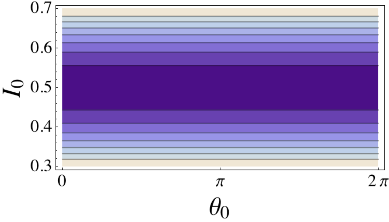
In Figure 1 we show two action-contour plots using the particle-in-wave Lagrangian/Hamiltonian

taking, specifically, $m=2$, $n=1$ (which also models a magnetic island at the $\mbox{$\,\iota\!\!$-}=0.5$ surface). The contours of the action were plotted for the 2-parameter family of $(1,2)$-periodic AGMin pseudo-orbits: Setting $p=1$, $q=2$, Eq. (22) under the boundary conditions Eqs. (23) was solved (using the Mathematica [24] routine NDSolve), for an array of initial conditions $\theta_{0}$ and $\dot{\theta}_{0}=I_{0}$ and plotted using Mathematica’s ListContourPlot.

Figure 1(a) shows the unperturbed case, $\epsilon=0$. In this case there is a horizontal valley of minima of $S$ on the rational invariant torus $I_{0}=\omega=1/2$, which is foliated by a family of $(1,2)$-periodic orbits (as $\delta S=0$ for each member of this family, all members must have the same value of $S$).

Figure 1(b) shows the case $\epsilon=0.002$, where all but two of the $\omega=1/2$ periodic orbits are destroyed because the action valley is not structurally stable under perturbation: the slightest ripple breaks it into minima and saddle points. Only two periodic orbits survive: the “minimax” orbit passing through the saddle points of $S$, which are seen to coincide with wave-frame-energy minima and hence this orbit is elliptically stable; and the “minimizing” orbits passing through the minima of $S$, which coincide with the saddle points of wave-frame energy (red curves, see below) and are thus hyperbolically unstable. The green curves are explained in Sec. 4.1.

By making a Galilean transformation to the wave frame the system in Eq. (24) can be made autonomous (it is isomorphic to the physical pendulum), and is thus integrable. The red solid curves in Fig. 1(b) show energy contours in the wave frame and are thus $t=0$ sections of invariant tori, which are seen to be of two distinct topological types—“librating” orbits within the island separatrix, and “rotating” orbits outside the separatrix. There is no diffeomorphic action-angle transformation continuously connected to the identity so this example, though integrable, is sufficient for illustrating the destruction of a primary invariant torus (see Remark 2), specifically the torus with the resonant rotation number $\omega=n/m=0.5$. [Note that, unlike the $(1,2)$-periodic pseudo-orbits used to construct the action-contour plots, each true orbit in general has a different rotation number.]

The path-pseudo-orbit method thus provides a visualization of the Poincaré–Birkhoff theorem [8], which shows that survival of a pair of minimizing and minimax orbits is generic after invariant torus with rational rotation number of an integrable system is destroyed by a perturbation that (in general) makes the system non-integrable. The minimizing and minimax orbits thus make a robust framework on which to build a theory of almost-invariant tori, as shown in Sec. 4.

In the alternative Hamiltonian phase-space formulation we introduce a Lagrange multiplier $\lambda(t)$ to take into account the constraint imposed by Eq. (18), which is difficult to implement explicitly. Then, to define $(p,q)$-periodic AGMin pseudo-orbits we extremize the functional

under independent variations of $\mathcal{I}$ and $\vartheta$. Varying Eqs. (16) and (17)

where ${\mathcal{I}}^{\prime}$ denotes $\mathcal{I}^{\prime}(t)$. Using these expressions and varying Eq (25) we find

Requiring $\delta f_{\rm ph}=0$ $\forall\,\delta\mathcal{I},\,\delta\vartheta$ gives the two Euler–Lagrange equations

where $\delta S_{\rm ph}/\delta\theta$ stands for the expression in Eq. (16).

These comprise one second-order and one first-order ordinary differential equation. With the constraint Eq. (18), which is a first-order o.d.e., we have three equations for the three dependent variables, $\vartheta$, $\cal I$ and $\lambda$. As we assume the twist condition Eq. (7) we can eliminate $\lambda$ between Eqs. (29) and Eq. (30) and replace them with the single third-order o.d.e.

The four arbitrary constants of the general solution are to be determined from the initial conditions and periodicity,

It is readily verified that the Hamiltonian pseudo-orbit defining equations Eq. (18), Eq. (31) and Eqs. (32) are equivalent to the Lagrangian defining equations Eq. (22) and Eqs. (23).

Figure 2 shows action plots for a particle in two waves (or field lines affected by islands on two rational surfaces), which is a nonintegrable system with Hamiltonian

where $V(\theta,t)\equiv-(1-\delta)\cos(m_{1}\theta-nt)-\delta\cos(m_{2}\theta-nt)$. Specifically, we take $n=1$, $m_{1}=2$ and $m_{2}=3$, which excites resonant islands at $\omega=1/2$ and $1/3$, and take $\delta=0.5$, $\epsilon=4\times 10^{-4}$. In the boundary conditions Eq. (23) or Eq. (32) we take $p=3$, $q=8$ so the path-pseudo-orbits have rotation number $\omega=3/8=0.375$. This fraction is a close rational approximant to the noble number $1-\gamma^{-1}=0.381966\ldots$, where $\gamma\equiv(1+\sqrt{5})/2$ is the golden mean (cf. Fig. 6 of Ref. 13). The AGMin pseudo-orbit defining equations were again solved using Mathematica’s NDSolve, but in Fig. 2 the results are displayed using ListPlot3D.

As the invariant torus at $\omega=1-\gamma^{-1}$ is very robust it should survive up to $\epsilon=O(1)$ so the pseudo-orbits of the neighboring $\omega=3/8$ almost-invariant-torus should all satisfy $\delta S\approx 0$ for the small value of $\epsilon$ we use. Thus the floor of the action valley should be almost level, as is observed, illustrating the potential of AGMin pseudo-orbits as a visualization tool for illustrating the Kolmogorov–Arnold–Moser (KAM) theorem [8, 25] and testing the existence of KAM tori.

To generalize the concept of invariant torus, we consider a 1-parameter family of $(p,q)$-periodic pseudo-orbits $\vartheta(t|\theta_{0})$, $2\pi$-periodic in $\theta_{0}$, such that $\vartheta(0|\theta_{0})\equiv\theta_{0}$. The almost-invariant tori studied in this paper are specifically those that can be built from from these pseudo-orbits.

However, before giving the full construction we first single out the pseudo-orbit starting at $\theta_{0}=0$ and consider the set formed from its images under the return map: $\{\vartheta(2\pi j|0)\!\!\mod 2\pi|j=0,1,\ldots,q-1\}$. We then rearrange this set to form the ordered set $\{\theta_{0}^{(0)}\equiv 0,\theta_{0}^{(1)},\ldots,\theta_{0}^{(q-1)}\}$, $\theta_{0}^{(i)}<\theta_{0}^{(i+1)}$ and extend it by defining $\theta_{0}^{(q)}\equiv 2\pi$ [as $\vartheta(2\pi q|0)$ and $\vartheta(0|0)$ are topologically equivalent by Eq. (9)].

Recalling that Def. 4 requires Eq. (1) to be satisfied, we can use Eq. (5) to determine $I$ and define a

In the above ${\rm d}_{\tau}\equiv\partial/\partial\tau$ denotes the time derivative along a given pseudo-orbit, i.e. with $\theta_{0}$ fixed. By restricting the range of $\theta_{0}$ we create a helical ribbon which, after wrapping around the torus $q$ times covers it completely. This is illustrated in Fig. 3 using a set of (1,2)-periodic AGMin-pseudo-orbits having the set of initial values shown by the solid green sinusoidal curve in Fig. 1(b). The dashed green sinusoidal curve in Fig. 1(b) shows the image of the solid curve under the return map—taken together these two green curves cover the interval $\theta_{0}\in[0,2\pi]$.

Note that the set of pseudo-orbits has been selected to include the minimizing and minimax true orbits as this is a natural feature of an almost-invariant torus (see Secs. 4.2 and 4.3). However this is not an essential feature of a pseudo-invariant torus, nor is the use of AGMin pseudo-orbits.

For simplicity (but see Remark 5 below) assume the configuration-space paths do not intersect in the $\theta,t$ covering space, so the map $\vartheta:\theta_{0}\mapsto\theta$ is a diffeomorphism for any value of $t$. As $\vartheta(t|\theta_{0})$ increases monotonically with $\theta_{0}$, when $t=0$, this remains true for all time:

Also, $I$ is a single-valued function of $\theta_{0}$ and $t$ and we can invert $\vartheta$ to make $I$ a graph over $\theta$ and $t$. That is, we can find a single-valued function $\rho$ such that $I=\rho(\theta,t)$. This is illustrated in Fig. 4.

Equations (34) clearly show that foliation by a given pseudo-orbit family is sufficient to specify a torus. Conversely, specification of an arbitrary trial torus $\mathcal{T}\in\Gamma_{3}$ implies a natural vector field in the tangent space at each point on the torus that locally defines a family of pseudo-orbits via a dynamical system. To see this, define $\mathcal{T}$ via a graph (for simplicity, but see Remark 5) of $I$ over the $\theta,t$ covering space $\mathbb{R}\times\mathbb{R}$

where $\rho$ is a $2\pi$-periodic function of $\theta$ and $t$. Combined with Eqs. (1) [implied by the constraint Eq. (18)] and (3) this implies the following two-dimensional vector field

Eliminating $\tau$ in favor of $t$ yields a nonlinear, first-order o.d.e. defining a family of solutions $\theta=\vartheta(t|\theta_{0})$, parametrized by the initial values $\theta_{0}$,

Thus we can define a phase-space pseudo-orbit $\theta=\vartheta(t|\theta_{0}),\;I=\mathcal{I}(t|\theta_{0})\equiv\rho(\vartheta(t|\theta_{0}),t)$ passing through each point of $\mathcal{T}$.

As illustrated in Fig. 1, when an invariant torus with rational rotation number is destroyed by a perturbation, two true orbits with the same rotation number survive: an “X-point” orbit that is a minimum of $S$, and an “O-point” orbit that is a minimax (saddle) point of $S$. The ghost-curve strategy is to join these two periodic orbits by a family of pseudo-orbits, labeled by a continuous parameter $T(\theta_{0})$, generated by flowing down the action gradient from minimax orbits to minimizing orbits. Below we describe this in configuration space and phase space.

We now define functionals $\varphi_{1}$ and $\varphi_{2}$ as surface integrals of powers of the action gradient over $\mathcal{T}$

It can be shown [see Eq. (51) below] that the surface integral linear in the action gradient vanishes identically, i.e. $\varphi_{1}\equiv 0$, which supports the interpretation of $\varphi_{1}$ as the net flux of extended phase space volume across $\mathcal{I}$. (In the case of magnetic fields this is the net magnetic flux [16], which is zero because of the absence of magnetic monopoles.)

Thus we must go to the “quadratic flux” $\varphi_{2}\geq 0$ before having a nontrivial measure of the invariance of $\mathcal{T}$ under the dynamics (equality to zero applying when $\delta S/\delta\theta=0$ on $\mathcal{T}$, i.e. if and only if it is an invariant torus). The quadratic flux is the analogue of the objective functional Eq. (19) for action-gradient-minimizing (AGMin) pseudo-orbits, but with the $L^{2}$ norm defined on tori rather than paths. Analogously, we define a quadratic-flux minimizing (QFMin) torus as follows.

References

- [1] P. J. Morrison, Hamiltonian description of the ideal fluid, Rev. Mod. Phys. 70 (1998) 467–521. doi:10.1103/RevModPhys.70.467.
- [2] Y. Elskens, D. F. Escande, Slowly pulsating separatrices sweep homoclinic tangles where islands must be small: an extension of classical adiabatic theory, Nonlinearity 4 (1991) 615–667. doi:10.1088/0951-7715/4/3/002.
- [3] R. L. Dewar, J. C.-C. Yap, Adiabatic wave-particle interaction revisited, Plasma Fusion Res. 4 (2009) 001–1–6, erratum: Plasma Fusion Res. 4, 005 (2009). doi:10.1585/pfr.4.001.
- [4] A. H. Boozer, Physics of magnetically confined plasmas, Rev. Mod. Phys. 76 (2004) 1071–1140. doi:10.1103/RevModPhys.76.1071.
- [5]
G. Metcalfe,
Applied
fluid chaos: Designing advection with periodically reoriented flows for micro
to geophysical mixing and transport enhancement, in: R. L. Dewar,
F. Detering (Eds.), Complex Physical, Biophysical and Econophysical Systems,
Vol. 9 of World Scientific Lecture Notes in Complex Systems, World
Scientific, Singapore, 2010, pp. 187–239, proceedings of the
Canberra International Physics Summer School, The Australian National
University, Canberra, 8–19 December 2008.
URL http://dl.dropbox.com/u/3064134/Metcalfe_AppliedChaos_2%010.pdf - [6] H. Goldstein, Classical Mechanics, 2nd Edition, Addison-Wesley, Reading, Mass., USA, 1980.
- [7] S. R. Hudson, J. Breslau, Temperature contours and ghost surfaces for chaotic magnetic fields, Phys. Rev. Lett. 100 (2008) 095001–1–4. doi:10.1103/PhysRevLett.100.095001.
- [8] J. D. Meiss, Symplectic maps, variational principles, and transport, Rev. Mod. Phys. 64 (1992) 795–848. doi:10.1103/RevModPhys.64.795.
- [9] S. R. Hudson, Calculation of cantori for hamiltonian flows, Phys. Rev. E 74 (2006) 056203–1–6. doi:10.1103/PhysRevE.74.056203.
- [10] S. R. Hudson, R. L. Dewar, Are ghost surfaces quadratic-flux-minimizing?, Phys. Lett. A 373 (2009) 4409–4415, erratum submitted Nov. 2009. doi:10.1016/j.physleta.2009.10.005.
- [11] G. Froyland, K. Padberg, Almost-invariant sets and invariant manifolds — connecting probabilistic and geometric descriptions of coherent structures in flows, Physica D 238 (2009) 1507—1523. doi:10.1016/j.physd.2009.03.002.
- [12]
J. D. Meiss, R. L. Dewar,
Minimizing flux, in: N. Joshi, R. L. Dewar (Eds.), Proceedings of
the CMA Miniconference on Chaos and Order, 1–3 February 1990, ANU, Canberra,
Australia, Centre for Mathematical Analysis, The Australian National
University, World Scientific, Singapore, 1991, pp. 97–103.
URL http://people.physics.anu.edu.au/~rld105/Dewar_Docs/_pr%eprints/Meiss_Dewar_91.pdf - [13] R. L. Dewar, J. D. Meiss, Flux-minimizing curves for reversible area-preserving maps, Physica D 57 (1992) 476–506. doi:10.1016/0167-2789(92)90015-F.
- [14] R. L. Dewar, A. B. Khorev, Rational quadratic-flux minimizing circles for area-preserving twist maps, Physica D 85 (1995) 66–78. doi:10.1016/0167-2789(95)00118-N.
- [15] C. Golé, Symplectic Twist Maps : Global Variational Techniques, World Scientific, Singapore, 2001.
- [16] S. R. Hudson, R. L. Dewar, Almost-invariant surfaces for magnetic field line flows, J. Plasma Phys. 56 (1996) 361–382. doi:10.1017/S0022377800019309.
- [17] D. del Castillo-Negrete, P. J. Morrison, Chaotic transport by Rossby waves in shear flow, Phys. Fluids A 5 (1993) 948–965. doi:10.1063/1.858639.
- [18] M. G. Davidson, R. L. Dewar, H. J. Gardner, J. Howard, Hamiltonian maps for Heliac magnetic islands, Australian J. Phys. 48 (1995) 871–886. doi:10.1071/PH950871.
- [19] R. L. Dewar, Optimal oscillation-center transformations, Physica D: Nonlinear Phenomena 17 (1985) 37–53. doi:10.1016/0167-2789(85)90132-0.
- [20] S. R. Hudson, R. L. Dewar, Analysis of perturbed magnetic fields via construction of nearby integrable fields, Phys. Plasmas 6 (1999) 1532–1538. doi:10.1063/1.873406.
- [21] S. R. Hudson, Destruction of invariant surfaces and magnetic coordinates for perturbed magnetic fields, Phys. Plasmas 11 (2004) 677–685. doi:10.1063/1.1640379.
- [22] D. E. Stewart, R. L. Dewar, Non-linear dynamics, in: T. R. J. Bossomaier, D. G. Green (Eds.), Complex Systems, Cambridge University Press, Cambridge, U.K., 2000, pp. 167–248. doi:10.2277/0521043719.
- [23] K. J. Palmer, Shadowing lemma for flows, Scholarpedia 4 (2009) 7918. doi:10.4249/scholarpedia.7918.
- [24]
Wolfram Research, Inc.,
Mathematica, Version 8, Wolfram Research, Champaign, Illinois, USA, 2010.
URL http://support.wolfram.com/mathematica/reference/genera%l/citing.html - [25] D. K. Arrowsmith, C. M. Place, An Introduction to Dynamical Systems, Cambridge University Press, Cambridge, U. K., 1991.
- [26]
R. L. Dewar, S. R. Hudson, A. M. Gibson,
Unified theory of ghost
and quadratic-flux-minimizing surfaces, J. Plasma Fusion Research SERIES 9
(2010) 487–490, in Proceedings of the 7th General Scientific Assembly of the
Asia Plasma and Fusion Association (APFA2009) and the Asia-Pacific Plasma
Theory Conference (APPTC2009), Aomori, Japan, October 27-30 2009.
URL http://www.jspf.or.jp/JPFRS/index_vol9-4.html - [27] R. S. MacKay, Greene’s residue criterion, Nonlinearity 5 (1992) 161–187. doi:10.1088/0951-7715/5/1/007.