Noise-induced behaviors in neural mean field dynamics
Abstract
The collective behavior of cortical neurons is strongly affected by the presence of noise at the level of individual cells. In order to study these phenomena in large-scale assemblies of neurons, we consider networks of firing-rate neurons with linear intrinsic dynamics and nonlinear coupling, belonging to a few types of cell populations and receiving noisy currents. Asymptotic equations as the number of neurons tends to infinity (mean field equations) are rigorously derived based on a probabilistic approach. These equations are implicit on the probability distribution of the solutions which generally makes their direct analysis difficult. However, in our case, the solutions are Gaussian, and their moments satisfy a closed system of nonlinear ordinary differential equations (ODEs), which are much easier to study than the original stochastic network equations, and the statistics of the empirical process uniformly converge towards the solutions of these ODEs. Based on this description, we analytically and numerically study the influence of noise on the collective behaviors, and compare these asymptotic regimes to simulations of the network. We observe that the mean field equations provide an accurate description of the solutions of the network equations for network sizes as small as a few hundreds of neurons. In particular, we observe that the level of noise in the system qualitatively modifies its collective behavior, producing for instance synchronized oscillations of the whole network, desynchronization of oscillating regimes, and stabilization or destabilization of stationary solutions. These results shed a new light on the role of noise in shaping collective dynamics of neurons, and gives us clues for understanding similar phenomena observed in biological networks.
keywords
mean field equations, neural mass models, bifurcations, noise, dynamical systemsAMS
34C15, 34C23, 60F99, 60B10, 34C25Introduction
The brain is composed of a very large number of neurons interacting in a complex nonlinear fashion and subject to noise. Because of these interactions, stimuli tend to produce coherent global responses, often with high reliability. At the scale of single neurons the presence of noise and nonlinearities often results in highly intricate behaviors. However, at larger scales, neurons form large ensembles that share the same input and are strongly connected, and at these scales, reliable responses to specific stimuli may arise. Such population assemblies (cortical columns or cortical areas) feature a very large number of neurons. Understanding the global behavior of these large-scale neural assemblies has been a focus of many investigations in the past decades. One of the main interests of large-scale modeling is to characterize brain function at the scale most non-invasive imaging techniques operate. Its relevance is also connected to the fact that anatomical data recorded in the cortex reveal its columnar organization at scales ranging from about to . These so-called cortical columns contain on the order of hundreds to hundreds of thousands of neurons, and are generally dedicated to specific functions. For example, in the visual cortex V1, they respond to preferred orientations in visual stimuli. These anatomical and functional organizations point towards the fact that a significant amount of information processing does not occur at the scale of individual neurons but rather corresponds to a mesoscopic signal arising from the collective dynamics of many interacting neurons.
In the computational neuroscience community, this problem has been mainly studied using approaches based on the statistical physics literature. Most models describing the emergent behavior arising from the interaction of neurons in large-scale networks have relied on continuum limits since the seminal works of Wilson and Cowan and Amari [3, 4, 57, 58]. Such models represent the activity of the network through a global variable, the population-averaged firing rate, which is generally assumed to be deterministic. Many analytical properties and numerical results have been derived from these equations and related to cortical phenomena, for instance in the case of the problem of spatio-temporal pattern formation in spatially extended models (see e.g. [18, 25, 27, 10]). This approach implicitly makes the assumption that the effect of noise vanishes in large populations.
However, increasingly many researchers now believe that the different intrinsic or extrinsic noise sources participate in the processing of information. Rather than having a pure disturbing effect there is the interesting possibility that noise conveys information and that this can be an important principle of brain function [46]. In order to study the effect of the stochastic nature of the firing in large networks, many authors strived to introduce randomness in a tractable form. A number of computational studies that successfully addressed the case of sparsely connected networks of integrate-and-fire neurons are based on the analysis of large assemblies that fire in an asynchronous regime [1, 5, 13]. Because of the assumption of sparse connectivity, correlations of the synaptic inputs can be neglected for large networks. The resulting asynchronous irregular states resemble the discharge activity recorded in the cerebral cortex of awake animals [20].
Other models have been introduced to account for the presence of noise in neuronal networks, such as the population density method and related approaches [16], allowing efficient simulation of large neuronal populations. In order to analyze the collective dynamics, most population density-based approaches involve expansions in terms of the moments of the resulting random variables, and the moment hierarchy needs to be truncated in order to get a closed set of equations, which can raise a number of technical issues (see e.g.[37]).
Yet other models of the activity of large networks are based on the definition of a Markov chain governing the firing dynamics of the neurons in the network, where the transition probability satisfies a differential equation called the master equation. Seminal works of the application of such modeling for neuroscience date back to the early 90s and have been recently developed by several authors [44, 24]. Most of these approaches are proved correct in some parameter regions using statistical physics tools such as path integrals [14] and Van-Kampen expansions [8]. They motivated a number of interesting studies of quasicycles [9] and power-law distribution of avalanche phenomena [7]. In many cases the authors consider one-step Markov chains, implying that at each update of the chain, only one neuron in the whole network either fires or stops firing, which raises biological plausibility issues. Moreover, analytical approaches mainly address the dynamics of a finite number of moments of the firing activity, which can also raise such issues as the well-posedness [37] and the adequacy of these systems of equations with the original Markovian model [51].
In the present study, we apply a probabilistic method to derive the limit behavior resulting from the interaction of an infinite number of firing-rate neurons nonlinearly interconnected. This approach differs from other works in the literature in that it relies on a description of the microscopic dynamics (neurons in the network), and does not make the assumption of a sparse connectivity. Our model takes into account the fact that cortical columns feature different populations. The approach consists in deriving the limit equations as the total number of neurons tends to infinity, based on results obtained in the field of large-scale systems of interacting particles. This problem has been chiefly studied for solving statistical physics questions, and has been a very active field of research in mathematics during the last decades [40, 23, 49, 48]. In general, the equations obtained by such rigorous approaches are extremely hard to analyze. They can be either seen as implicit equations in the set of stochastic processes, or as non-local partial differential equations on the probability distribution through the related Fokker-Planck equations. But in both cases, understanding the dynamics of these equations is very challenging, even for basic properties such as the existence and uniqueness of stationary solutions and a priori estimates [33]. It appears even more difficult to understand qualitatively the effects of noise on the solutions and to interpret them in terms of the underlying biological processes.
In the present article we aim at answering some of these questions. In the case we address, the problem is rigorously reducible to the analysis of a set of ordinary differential equations. This is because the solution of the mean field equations is a Gaussian process. It is therefore completely determined by its first two moments which we prove to be the solutions of ordinary differential equations. This allows us to go much deeper into the analysis of the dynamical effects of the parameters, in particular those related to the noise, and to understand their influence on the solutions. The analysis of this Gaussian process also provides a rich amount of information about the non-Gaussian solution of the network when its size is large enough.
The paper is organized as follows. In the first section we deal with the modeling, the derivation of the mean field equations and of the related system of ordinary differential equations. We then turn in section 2 to the analysis of the solutions of these equations and the influence of noise. We show in details how noise strongly determines the activity of the cortical assembly. We then return to the problem of understanding the behavior of finite-size (albeit large) networks in section 3 and compare their behavior with those of the solutions of the mean field equations (infinite-size network). The analysis of the network behaviors in the different regimes of the mean field equations provides an interpretation of the individual behaviors responsible for collective reliable responses. This has a number of consequences that are developed in section 4.
1 Model and mean field equations
In all the article, we work in a complete probability space assumed to satisfy the usual conditions.
We are interested in the large scale behavior arising from the nonlinear coupling of a large number of stochastic diffusion processes representing the membrane potential of neurons in the framework of rate models (see e.g. [19, 30]). Hence the variable characterizing the neuron state is its firing rate, that exponentially relaxes to zero when it receives no input, and that integrates both external input and the current generated by its neighbors. The network is composed of neural populations that differ by their intrinsic dynamics, the input they receive and the way they interact with the other neurons. Each population is composed of neurons, and we assume that the ratio converges to a constant in when the total number of neurons becomes arbitrarily large. We define the population function that maps the index of any neuron to the index of the population neuron belongs to: .
For any neuron in population , the membrane potential has a linear intrinsic dynamics with a time constant . The membrane potential of each neuron returns to zero exponentially if it receives no input. The neuron in population receives an external current, which is the sum of a deterministic part and a stochastic additive noise driven by independent adapted Brownian motions modulated by the diffusion coefficients . This additive noise term accounts for different biological phenomena [2], such as intrinsically noisy external input, channel noise [56] produced by the random opening and closing of ion channels, thermal noise and thermodynamic noise related to the discrete nature of charge carriers.
Neurons also interact through their firing rates, classically modeled as a sigmoidal transform of their membrane potential. These sigmoidal functions only depend on the population the neuron belongs to: . The functions are assumed to be smooth (Lipchitz continuous), increasing functions that tend to at and to at . The firing rate of the presynaptic neuron , multiplied by the synaptic weight , is an input current to the postsynaptic neuron . We classically assume that the synaptic weight is equal to . In practice this synaptic weight randomly varies depending on the local properties of the environment. Models including this type of randomness are not covered in this paper. The scaling assumption is necessary to ensure that the total input to a neuron does not depend on the network size.
The network behavior is therefore governed by the following set of stochastic differential equations:
| (1) |
These equations represent a set of interacting diffusion processes. Such processes have been studied for instance by McKean, Tanaka and Sznitman among others [40, 50, 49, 48]. This case is simpler than the different cases treated in [53] where the intrinsic dynamics of each individual diffusion is nonlinear.
We aim at identifying the limit in law of the activity of finite sets of neurons in the network as the number of neurons tend to infinity. The identification of this law will imply the fact that the system satisfies the propagation of chaos property. This property states that, provided the initial conditions are independent and identically distributed for all neurons of each population (initial conditions are said to be chaotic** * Note that the term chaos is understood here in the statistical physics sense as the Boltzmann’s molecular chaos (”Stoßzahlansatz”), corresponding to the independence between the velocities of two different particles before they collide. This is very different from the notion of chaos in deterministic dynamical systems. ), then in the limit , all neurons behave independently, and have the same law which is given by an implicit equation on the law of the limiting process (the chaos of the initial condition is propagated for all time ). In details, the law of for any fixed and , converges towards when , where denotes the law of the solution of equation (2) corresponding to population .
This convergence and the limit equations are the subject of the following theorem:
Theorem 1.
Let a fixed time. Under the previous assumptions, we have:
- (i).
The process for in population , solution of equation (1), converges in law towards the process solution of the mean field implicit equation:
(2) as a process for , in the sense that there exists distributed as such that
where is a finite quantity depending on the time horizon and on the parameters of the system. As a random variable, it converges uniformly in time in the sense that:
where does not depend on time. In equations (2), the processes are independent Brownian motions.
- (ii).
Equation (2) has a unique (trajectorial and in law) solution which is square integrable.
- (iii).
The propagation of chaos applies.
Note that the expectation term in equation (2) is the classical expectation of a function of a stochastic process. In details, if is the probability density of , is equal to .
The proof of this theorem essentially uses results from the works of Tanaka and Sznitman, summarized in [48]. A distinction with these classical results is that the network is not totally homogeneous but composed of distinct neural populations. Thanks to the assumption that the proportion of neurons in each population is non-trivial (), the propagation of chaos occurs simultaneously in each population yielding our equations, as it is shown in a wider setting in [53]. The main deep theoretical distinction is that the theorem claims a uniform convergence in time: most of the results proved in the kinetic theory domain show propagation of chaos properties and convergence results only for finite time intervals, and convergence estimates diverge as the interval grows. Uniform propagation of chaos is an important property as commented in [17], and particularly in our case as we will further comment. Methods to prove uniformity are generally involved (see e.g. [41] where uniformity is obtained for certain models using a dual approach based on the analysis of generator operators). Due to the linearity of the intrinsic dynamics, we provide here an elementary proof of this property in our particular system.
Proof.
The existence and uniqueness of solutions can be performed in a classical fashion using Picard iterations of an integral form of equation (2) and a contraction argument. The proof of the convergence towards this law, and of the propagation of chaos can be performed using Sznitman’s powerful coupling method (see e.g. [48], method which dates back from Dobrushin [23]), that consists in exhibiting an almost sure limit of the sequence of processes as goes to infinity by coupling the mean field equation with the network equation as follows. We define the different independent processes solution of equation (2) driven by the same Brownian motion as involved in the network equation (1), and with the same initial condition as neuron in the network. It is clear that these processes are independent (since the are pairwise independent) and have the same law as the solution of the mean field equation (2). The almost sure convergence of towards will therefore imply the convergence in law towards the mean field equation. For a neuron belonging to population , we have:
We have, denoting by the maximal value of :
| (3) |
where . is the largest Lipschitz constant of the sigmoids , and , quantity upperbounded, for sufficiently large, by .
Since the righthand side of (3) does not depend on the index , taking the maximum with respect to and the expected value of both sides of (3), we obtain
| (4) |
Since the random variables are independent and centered (i.e. have a null expectation), using the fact that the sigmoids take their values in the interval , using Cauchy-Scwartz and posing , we have:
By Cauchy-Schwartz inequality, we can upperbound the second term of the righthand side of inequality (4) by . Therefore, defining , and we have:
implying, using Gronwall’s lemma,
This inequality readily yields the almost sure convergence of towards as goes to infinity, uniformly in time, and hence convergence in law of towards .
The almost sure convergence of (considered as a process) towards can be proved in a similar fashion. Indeed, upperbounding the exponential term in (3) by and taking the supremum, it is easy to see that:
using the fact that:
using the independence of the and Cauchy-Schwartz inequality. This last estimate readily implies, using Gronwall’s inequality:
The propagation of chaos property (iii) stems from the almost sure convergence of towards which are independent, as a process and uniformly for fixed time, and is proved in a similar fashion. ∎
The equations (2), which are implicit stochastic differential equations, describe the asymptotic behavior of the network. However, the characterization and simulation of their solutions is a challenge. Fortunately, due to their particular form in our setting, these equations can be substantially simplified. Indeed, under some weak assumptions, the solutions of the mean field equations are shown to be Gaussian, allowing to exactly reduce the dynamics of the mean field equations to the study of coupled ordinary differential equations as we now show.
Proposition 2.
Let us assume that is a P-dimensional Gaussian random variable. We have:
-
The solutions of the P mean field equations (2) with initial conditions are Gaussian processes for all time.
-
Let denote the mean vector of and its variance. Let also denote the expectation of for a Gaussian random variable of mean and variance . We have:
(5) with initial conditions and . In equation (5), the dot denotes the differential with respect to time.
Proof.
The unique solution of the mean field equations (2) starting from a square integrable initial condition measurable with respect to can be written in the form:
| (6) |
We observe that if is a Gaussian random variable, then the righthand side of (6) is necessarily Gaussian as the sum of a scaled version of this random variable, a deterministic term and an Itô integral of a deterministic function, and hence so is the solution of the mean field equation. Its law is hence characterized by its mean and covariance functions. The formula (6) involves the expectation , which, because of the Gaussian nature of , only depends on and , and is denoted by . Taking the expectation of both sides of the equality (6), we obtain the equation satisfied by the mean of the process :
Taking the variance of both sides of the equality (6), we obtain the following equation:
and this concludes the proof. ∎
Remark 1.3.
- •
In order to fully characterize the law of the process , we need to compute the covariance matrix function for and in . For this covariance is clearly zero using equation (6), and we have:
(7) for , hence only depends on the parameters of the system and is in particular not coupled to the dynamics. The description of the solution given by equations (5) is hence sufficient to fully characterize the solution of the mean field equations (2).
- •
The uniformity in time of the propagation of chaos has deep implications in regard of equations (5). Indeed, we observe that the solution of the mean field equation is governed by the mean of the process, the expectation being a deterministic function depending on the parameters of the system. The uniformity in particular implies that, for in population :
(8) implying uniform convergence of the empirical mean, as a function of time, towards .
- •
If is not Gaussian, the solution of equation (2) asymptotically converges exponentially towards a Gaussian solution. The important uniformity convergence property towards the mean field equations ensures that the Gaussian solution is indeed the asymptotic regime of the network, which strengthens the interest of the analysis of the differential system (5).
The functions depend on the choice of the sigmoidal transform. A particularly interesting choice is the sigmoidal function†† † We emphasize that in this article, the function is understood as the repartition function of a standard Gaussian random variable, i.e. . In particular, this function is always positive. It is distinct from the usual definition of the function corresponding to . This function is not always positive (hence not a good rate function) and is related to our function through the formula: . . In that case we are able to express the function in closed form, because of the following lemma:
Lemma 1.4.
In the case where the sigmoidal transforms are of the form , the functions involved in the mean field equations (5) with a Gaussian initial condition take the simple form:
| (9) |
Proof 1.5.
The proof is given in Appendix A.
In summary, we have shown that, provided that the initial conditions of each neuron are independent and Gaussian, the large-scale behavior of our linear model is governed by a set of ordinary differential equations (theorem 1 and proposition 2). This is very interesting since it reduces the study of the solutions to the very complex implicit equation (2) bearing on the law of a process to a much simpler setting, ordinary differential equations. As shown below this allows us to understand the effects of the system parameters on the solutions. For this reason we assume from now on that the initial condition is Gaussian, and focus on the effect of the noise on the dynamics.
2 Noise-induced phenomena
In this section we mathematically and numerically study the influence of the noise levels on the dynamics of the neuronal populations. Thanks to the uniform convergence of the empirical mean towards the mean of the mean field system (equation (8)) and the propagation of chaos property for the network process, it is relevant to study such phenomena through the thorough analysis of the solutions of the mean field equations given by the ODEs (5). This is what we do in the present section.
As observed in equation (5), in the case of a Gaussian initial condition, the equation of the variance is decoupled from the equation on the mean in (5). The variance satisfies an autonomous equation:
which is easily integrated as:
is therefore independent of the mean . This implies that the equations on are a set of non-autonomous ordinary differential equations.
These ordinary differential equations are similar to those of a single neuron. They differ in that the terms in the sigmoidal functions depend on the external noise levels . They read:
hence the slope and the threshold are scaled by a time-varying coefficient which is always smaller than one.
We now focus on the stationary solutions when the noise parameter does not depend upon time. In that case, the variance is equal to:
and converges exponentially fast towards the constant value . Asymptotic regimes of the mean field equations are therefore Gaussian random variables with constant standard deviation. Their mean is solution of the equation:
In other words, the presence of noise has the effect of modifying the slope and the threshold of the sigmoidal function, but the type of the equations is the same as that of the equation of each individual neuron or cortical column, it is a rate equation.
We observe that the larger the noise amplitude , the smaller the slope of the sigmoidal transform. Noise has the effect of smoothing the sigmoidal transform. This will have a strong influence on the bifurcations of the solutions to the mean field equations and hence on the behaviors of the system. We demonstrate these effects for two simple choices of parameters in one- and two-population networks.
2.1 The external noise can destroy a pitchfork bifurcation
Let us start by considering the case of a one-population network. We drop the index since no confusion is possible. We assume for simplicity that the threshold of the sigmoid is null and that the time constant is equal to one. By doing so, we do not restrict the generality of the study, since can be eliminated by rescaling the time and can be absorbed into by a simple change of origin for . The network equations read:
and we are interested in the limit in law of their solutions as the number of neurons tends to infinity.
In order to analytically study the effect of the parameter , we set . In that case, and in the absence of noise, the solution is a fixed point of the network equations. The following proposition characterizes their solutions in the deterministic and stochastic cases.
Proposition 2.6.
In a non-stochastic finite-size network, the null solution is:
- •
stable if or if and ,
- •
unstable for and .
- •
For , the system undergoes a pitchfork bifurcation at .
In the mean field limit of the same stochastic network, the pitchfork bifurcation occurs for a new value of if and . Furthermore the null solution is:
- •
stable if:
-
or
-
and (large noise case) or
-
, and ,
-
- •
unstable for , and , and
- •
the system undergoes a pitchfork bifurcation at when and .
This proposition is a bit surprising at first sight. Indeed, it says that noise can stabilize a fixed point which is unstable in the same non-stochastic system. Even more interesting is the fact that if the system is driven by a sufficiently large noisy input, the zero solution will always stabilize. It is known, see, e.g., [38], that noise can stabilize the fixed points of a deterministic system of dimension greater than or equal to . The present observation extends these results to a one-dimensional case, in a more complicated setting because of the particular, non-standard, form of the mean field equations. Also note that this proposition provides a precise quantification of the value of the parameter that destabilizes the fixed point. This is a stochastic bifurcation of the mean field equation (a P-bifurcation –P for phenomenological– in the sense of [6]). This estimation will be used as a yardstick for the evaluation of the behavior of the solutions to the network equations in section 3.
Proof 2.7.
We start by studying the finite-size deterministic system. In the absence of noise, it is obvious because of our assumptions that the solution for all is a fixed point of the network equations. At this point, the Jacobian matrix reads , where is the identity matrix and is the matrix with all elements equal to one. The matrix is diagonalizable, all its eigenvalues are equal to zero except one which is equal to . Hence, all eigenvalues of the Jacobian matrix are equal to , except one which is equal to . The solution where all are equal to zero in the deterministic system is therefore stable if and only if . The eigenvalue corresponding to the destabilization corresponds to the eigenvector whose components are all equal to . Interestingly, this vector does not depend on the parameters, and therefore it is easy to check that at the point the system loses stability through a pitchfork bifurcation. Indeed, because of the symmetry of the function, the second derivative of the vector field projected on this vector vanishes, while the third derivative does not (it is equal to ).
Considering now the stochastic mean field limit, the stationary mean firing rate in that case is solution of the equation:
Here again, the null firing rate point is a fixed point of the mean field equations, and it is stable if and only if . The remaining of the proposition readily follows from the fact that the stability changes at where .
Note that the results in this proposition only depend on and its effect on the slope of the sigmoid. It is a general phenomenon that goes beyond the example in this section: increasing decreases the slope of the sigmoidal transform and the threshold. In section 3 we will see that this phenomenon can be observed at the network level, and a good agreement will be found between the finite-size network behavior and the predictions obtained from the mean field limit.
We now turn to an example in a two-dimensional network, where the presence of oscillations will be modulated by the noise levels.
2.2 The external noise can destroy oscillations
The same phenomenon of nonlinear interaction between the noise intensity and the sigmoid function can lead, in higher dimensions, to more complex phenomena such as the disappearance or appearance of oscillations. In order to study phenomena of this type, we instantiate a simple two-populations network model in which, similarly to the one-dimensional case, all the calculations can be performed analytically. The network we consider consists of an excitatory population, labeled , and an inhibitory population, labeled . Both populations are composed of the same number of neurons ( is assumed in all the subsection to be even), and have the same parameters , and . We choose for simplicity the following connectivity matrix:
and we assume that the inputs are set to and . The zero solution where all neurons have a zero voltage is a fixed point of the equations whatever the number of neurons in each population. We have the following result:
Proposition 2.8.
In the deterministic finite-size network, the null solution is:
- •
stable if or if and ,
- •
unstable for and and the solutions are oscillating on a periodic orbit.
- •
For the system undergoes a supercritical Hopf bifurcation at .
In the mean field limit of the same stochastic network, the Hopf bifurcation occurs for a new value of the slope parameter . Furthermore the null solution is:
- •
stable if:
-
or
-
and (“large noise case”) or
-
, and ,
-
- •
unstable for , and , and the system features a stable periodic orbit.
- •
The system undergoes a supercritical Hopf bifurcation at when and .
Note that proposition 2.8 is quite similar to proposition 2.6, the qualitative difference being that the system is oscillating. The proof is closely related and is presented in less details.
Proof 2.9.
In the deterministic network model, the Jacobian matrix at the null equilibrium can be written as
where denotes the Kronecker product (see e.g. [43, 11]), i.e. the Jacobian matrix is built from blocs of size and each of these blocks is a copy of . The eigenvalues of a Kronecker product of two matrices are all possible pairwise products of the eigenvalues of the matrices. Since the eigenvalues of are equal to where , and as noted previously, the eigenvalues of are with multiplicity and with multiplicity , we conclude that the Jacobian matrix has eigenvalues equal to , and two eigenvalues equal to . The null equilibrium in this deterministic system is therefore stable if and only if the real parts of all eigenvalues are smaller than , viz. . Therefore, for a fixed , the system has a bifurcation at . The analysis of the eigenvectors allows to check the genericity and transversality conditions of the Hopf bifurcation (see e.g. [32]) in a very similar fashion to the proof of proposition 2.6.
In the mean field model, the same analysis applies and, as in the one-dimensional case, the bifurcation point is shifted to when this value is well-defined, which concludes the proof of the proposition 2.8.
We have therefore shown that noise can destroy the oscillations of the network. The results of propositions 2.6 and 2.8 are summarized in figure 1.
An even more interesting phenomenon is that noise can also produce regular cycles in the mean part of the solution of the mean field equations, for parameters such that the deterministic system presents a stable equilibrium. This is the subject of the following section.
2.3 The external noise can induce oscillations
In order to uncover further effects of the noise on the dynamics, we now turn to the numerical study of a two-populations network including excitation and inhibition. The time constant , sigmoidal transforms , noise intensity and the initial condition on the variance are chosen identical for both population. Under these hypotheses, the variances of the two populations are identical and denoted by . We further assume that , and hence the mean field nonlinear function is given by lemma 1.4. The connectivity matrix is set to . The input currents and are considered constant. The mean field equations in that case read:
The codimension two bifurcation diagram of the system for is displayed in Figure 2 (qualitative results turn out to change smoothly when is also allowed to vary). It features two cusps (CP) and one Bogdanov-Takens (BT) bifurcations. In addition to these local bifurcations, we observe that the Hopf bifurcation manifold (shown in pink in Figure 2) and the saddle-homoclinic bifurcation curve (green line) present a turning point, i.e. change monotony as a function of .
The diagram can be decomposed into different regions depending on the dynamical features (number and stability of fixed points or cycles): the “trivial” zone where the system features a unique stable fixed point (not colored), a zone with 2 unstable and 1 stable fixed point (green zone (a)) separated by the saddle-homoclinic bifurcation curve from region (b) (yellow) where an additional stable cycle exists. Zone (c) (orange) features a stable cycle and an unstable fixed point, and zone (d) (green) features 2 stable and 1 unstable fixed points.
Let us for instance fix . As is increased, several noise-induced transitions occur leading the system successively in zone (a), (b), (c) and the trivial zone (see codimension one bifurcation diagram in Figure 2 (i)). In details, for small noise levels the system features a unique stable fixed point (zone (a)). A family of large amplitude and small frequency periodic orbits appears from the saddle-homoclinic bifurcation yielding a bistable regime (zone (b)) before the stable fixed point disappears through a saddle-node bifurcation (zone (c)). The amplitude of these cycles progressively decreases and their frequency progressively increases as the noise intensity is increased, and they eventually disappear through a supercritical Hopf bifurcation leading to the trivial behavior with a single fixed point. We emphasize here the fact that the sudden appearance of large amplitude slow oscillations can be compared to epileptic spikes, which are characterized by the presence of collective oscillations of large amplitude and small frequency suddenly appearing in a population of neurons (see [52]). This comparison turns out to be relevant from the microscopic viewpoint: network simulations of section 3 will indeed show a sudden synchronization of all neurons at this transition.
The diagram can also be decomposed into six different noise levels intervals (labels (A) through (F) in Figure 2) corresponding to qualitatively different codimension 1 bifurcation diagrams as is varied (the six corresponding bifurcation diagrams are presented in appendix B). The presence of these different zones illustrate how the noise influences the response of the neural assembly to external inputs. For instance, for large enough, no cycles exist whatever (zones (E-F)), whereas for small enough (zones A-D), cycles always exist for some values of the input. Such partitions may provide an experimental design for evaluating a noise level range as a function of the observed dynamics when varying the input to the excitatory population for instance.
3 Back to the network dynamics
Thus far, we studied the dynamics of the mean field equations representing regimes of the network dynamics in the limit where the number of neurons is infinite. We now compare the regimes identified in this analysis with simulations of the finite-size stochastic network. We are particularly looking for potential finite-size effects, namely qualitative differences between the solutions to the network and the mean field equations. This will provide us with information about the accuracy of an approximation of the network dynamics by the mean field model, as function of the size of the network.
3.1 Numerical Simulations
Numerical simulations of the network stochastic differential equations (1) are performed using the usual Euler-Maruyama algorithm (see e.g. [39, 38]) with fixed time step (less than ) over an interval . In order to observe oscillations, we choose between and . The simulations are performed with Matlab®, using a vectorized implementation that has the advantage to be very efficient even for large networks. The computation time stays below s for networks up to neurons, and appears to grow linearly with the size of the network once the cache memory saturates (see Figure 3). For instance, for , , the simulation of a neurons network takes s, and for neurons, s on a HP Z800 with 8 Intel Xeon CPU E5520 @ 2.27 GHz 17.4 Go RAM. The main limitation preventing the simulation of very large networks is the amount of memory required for the storage of the trajectories of all neurons.
An important property arising from theorem 1 is that asymptotically, neurons behave independently and have the same probability distribution. In our numerical simulations, we will make use of this asymptotic independence and, in order to evaluate an empirical mean of the process related to a given neuron in population , will compute both the empirical mean over all neurons in that population and a mean over different independent realization of the process. This method allows to reduce sensitively the number of independent simulations in order to obtain a given precision in the empirical mean evaluation.
3.2 A one population case
We start by addressing the case discussed in section 2.1 where we showed analytically that the loss of stability of the null fixed point as the slope of the sigmoid was varied depended on the noise parameter . We now investigate numerically the stability of the fixed point of the network equations. In order to check for the presence of a pitchfork bifurcation, we compute, for each value of the noise and for each value of the slope of the sigmoid, an estimated value of the mean of the membrane potential. This estimate is calculated by averaging out over independent realizations the empirical mean of the membrane potentials of all neurons in the network at the final time. We display the average value then compare these simulations with those of the mean field equations stopped at the same time as the network. We observe that both are very similar and show some differences with the bifurcation diagram that corresponds to the asymptotic regimes.
The results of the simulations, where we have also varied , are shown in Figure 4 and reveal two interesting features. First, because we simulate over a finite time, we tend to smooth the pitchfork bifurcation: this is perceptible for both the network and the mean field equations. Second, we observe that the loss of stability of the zero fixed point arises at the value of predicted by the analysis of the mean field equations for networks as small as neurons. The value reached by the simulations of the network is very close to that related to the mean field equation as soon as becomes greater than .
3.3 Two populations case and oscillations
We now investigate the case shown in Figure 2 (i) where cycles are created (through homoclinic bifurcation) or destroyed (through Hopf bifurcation) as the additive noise intensity parameter is increased.
Looking at Figure 2(i), we observe that for , stable periodic orbits coexist with stable fixed points in the mean field system. For smaller values of , the mean field system features a unique stable fixed point, while for , it features a unique stable limit cycle, and for , the dynamics is reduced to a unique attractive fixed point. Numerical simulations confirm this analysis. Let us for instance illustrate the fact that the network features the bistable regime, the most complex phenomenon. Figure 5 shows simulations of a network composed of neurons in each population (time step , total time ). Depending on the mean and on the standard deviation of the initial condition, we observe that the network either converges to the mean field fixed point or the periodic orbit. Both mean field equations show very close behaviors.
In the fixed point regime corresponding to small values of we observe that the membrane potential of every neuron randomly varies around the value corresponding to the fixed points of the mean field equation (see Figure 6, cases (a) and (b))), with a standard deviation that converges toward the constant value as predicted by the mean field equations. The empirical mean and standard deviation of the voltages in the network show a very good agreement with the related mean field variables. For larger values of corresponding to the oscillatory regime (Figure 6, cases (c) and (d)), all neurons oscillate in phase. These synchronized oscillations yield a coherent global oscillation of the network activity. The statistics of the network are again in good agreement with the mean field solution. The standard deviation converges towards the constant solution of the mean field equation. This is visible at the level of individual trajectories, that shape a “tube” of solutions around the periodic mean field solution, whose size increases with . The empirical means accurately match the regular oscillations of the solution of the mean field equation. A progressive phase shift is observed, likely to be related with the time step involved in the simulation. Note that the phase does not depend on the realization. Indeed, according to theorem 1, the solution of the mean field equations only depends on the mean and the standard deviation of the Gaussian initial condition, which therefore governs the phase of the oscillations on the limit cycle (see Figure 7).
In the fixed point regime related to large values of , very noisy trajectories are obtained because of the levels of noise involved (see Figure 6, cases (e) and (f)). Though the individual neurons show very fluctuating trajectories, the empirical mean averaged out over all neurons in the network fits closely the mean field fixed point solution.
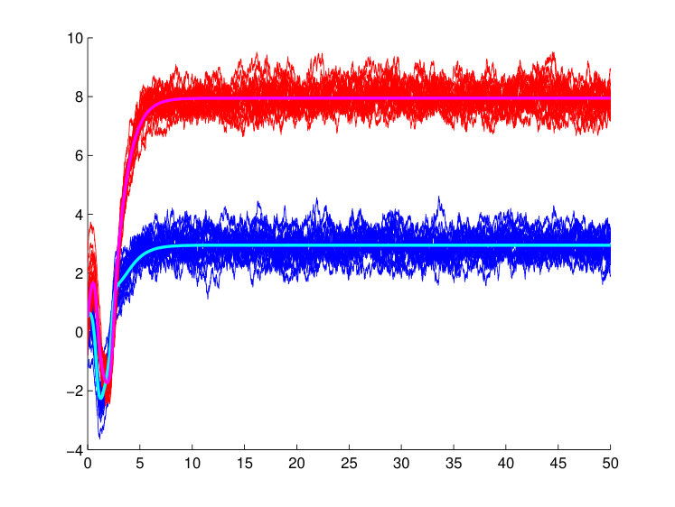
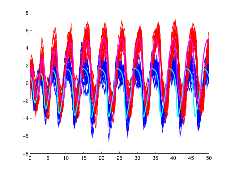
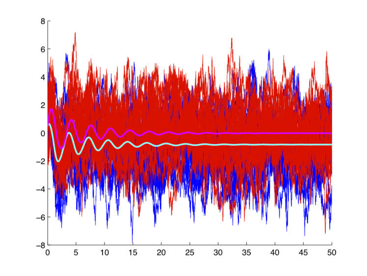
Eventually, we study the switching between a fixed-point regime and an oscillatory regime by extensively simulating the neurons network for different values of and computing the Fourier transform of the empirical mean (see Figure 8). The three-dimensional plots show that the appearance and disappearance of oscillations occur for the same values of the parameter as in the mean field limit, and the route to oscillations is similar: at the homoclinic bifurcation in the mean field system, arbitrarily small frequencies are present, this is also the case for the finite-size network. At the value of related to the Hopf bifurcation, the system suddenly switches from a non-zero frequency to a zero frequency in a form that is very similar to the network case. Therefore we conclude that the mean field equations accurately reproduce the network dynamics for networks as small as neurons, and hence provide a good model, simple to study, for networks of the scale of typical cortical columns. As a side remark, we note that at a homoclinic bifurcation of the mean field system, very small frequencies appear and a precise description of the spectrum of the network activity would require very large simulation times to uncover precisely the spectrum at this point, even more so since the large standard deviation of the process disturbs the synchronization. In a forthcoming study focusing on mean field equations arising in a similar system including dynamically fluctuating synaptic coefficients, an interesting additional phenomenon will appear: in that case, the standard deviation variable will be coupled to the mean, and this coupling will result in sharpening the synchronization.

We conclude this section by discussing heuristic arguments explaining the observed regular oscillations. Let us start by stating that this phenomenon is a pure collective effect: indeed, two-neurons networks (one per population) do not present such regular oscillations as noise is varied. We observe that individual trajectories of the membrane potential of a 2-neurons networks for small noise levels stay close to the deterministic fixed point. However, when noise is increased, the system starts making large excursions with a typical shape resembling the cycle observed in the mean field limit, and these excursions occur randomly. Such excursions are typical of the presence of a homoclinic deterministic trajectory: when perturbed, the system catches the homoclinic orbit responsible for such large excursions. The codimension one bifurcation diagram of the 2-neurons system indeed illustrates the presence of a homoclinic orbit as a function of (see diagram 2, and Figure 12 (A))‡‡ ‡ Indeed, the mean field equations with are precisely the equations of a two-neurons network since in that case .. Noise can be heuristically seen as perturbing the deterministic value of . For sufficiently small values of the noise parameter, the probability of to visit regions corresponding to the presence of a cycle is small. But as the noise amplitude is increased, this probability becomes non-negligible and individual trajectories will randomly follow the stable cycle. Such excursions produce large input to the other neurons which will either be inhibited or excited synchronously at this time, a phenomenon that may trigger synchronized oscillations if the coupling is strong enough and the proportion of neurons involved in a possible excursion large enough. If the noise parameter is too large, the limit cycle structure will be destroyed.
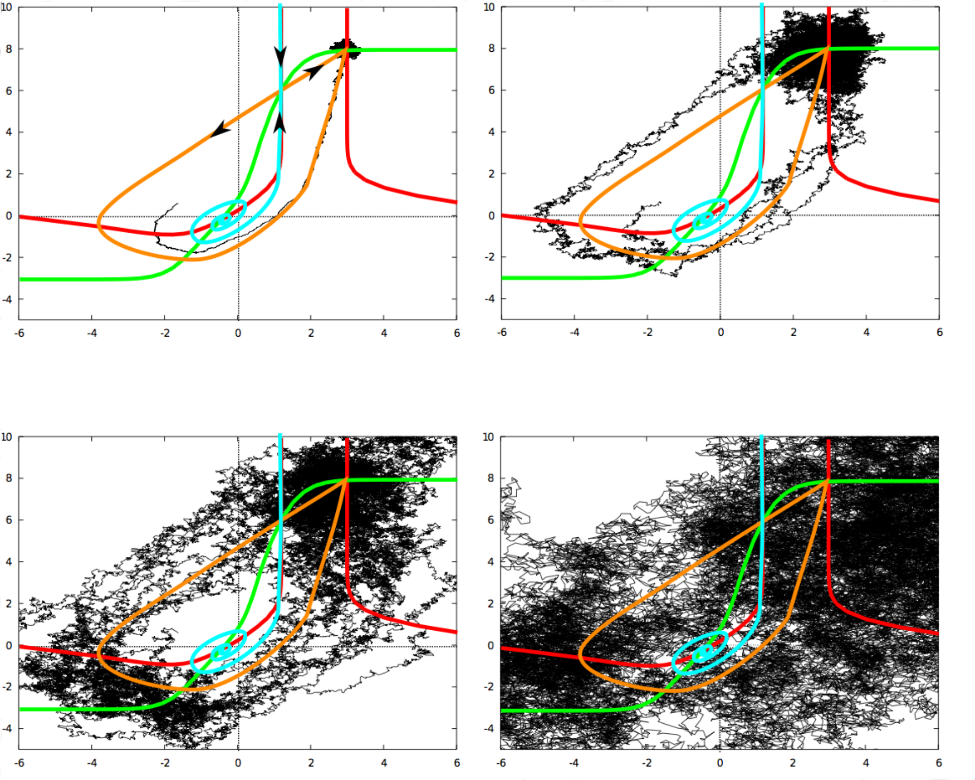
Another way to understand this phenomenon consists in considering the phase plane dynamics of the two-neurons network with no noise (see Figure 9). The system presents three fixed points, one attractive, one repulsive, and a saddle. The unstable manifold of the saddle fixed point connects with the stable fixed point in an heteroclinic orbit. The stable manifold of the saddle fixed point is a separatrix between trajectories that make small excursions around the stable fixed point, and those related to large excursions close to the heteroclinic orbit. As noise is increased, the probability distribution of each individual neuron, centered around the stable fixed point, will grow larger until it crosses the separatrix with a non-negligible probability, resulting in the system randomly displaying large excursions around the heteroclinic cycle. The fact that a homoclinic path to oscillations is found in the mean field limit can be accounted for by these observations, considering the fact that crossing the separatrix, when noise is of small amplitude, can take an arbitrary long time. The rhythmicity of the oscillations we found and the synchronization are related to the coupling in a complex interplay with the probability of large excursions. These heuristic arguments require a thorough mathematical analysis that is outside the scope of the present paper.
4 Discussion
In this article, we have been interested in the large-scale behavior of networks of firing rate neuron models. Using a probabilistic approach, we addressed the question of the behavior of neurons in the network as its size tends to infinity. In that limit, we showed that all neurons behaved independently and satisfied a mean field equation whose solutions are Gaussian processes such that their mean and variance satisfy a closed set of nonlinear ordinary differential equations. Uniform convergence properties were obtained.
We started by studying the solutions of the mean field equations, in particular their dependence with respect to the noise parameter using tools from dynamical systems theory. We showed that the noise had non-trivial effects on the dynamics of the network, such as stabilizing fixed points, inducing or canceling oscillations. A codimension two bifurcation diagram was obtained when simultaneously varying an input parameter and the noise intensity, as well as simultaneously varying a total input connectivity parameter and the noise intensity. The analysis of these diagrams yielded several qualitatively distinct codimension one bifurcation diagrams for different ranges of noise intensity. Noise therefore clearly induces transitions in the global behavior of the network, structuring its Gaussian activity by inducing smooth oscillations of its mean.
These classes of behaviors were then compared to simulations of the original finite-size networks. We obtained a very good agreement between the simulations of the finite-size system and the solution of the mean field equations, for networks as small as a few hundreds to few thousands of neurons. Transitions between different qualitative behaviors of the network matched precisely the related bifurcations of the mean field equations, and no qualitative systematic finite-size effects were encountered. Moreover, it appears that the convergence of the solution to a Gaussian process as well as the propagation of chaos property happen for quite small values of , as illustrated in Figure 10. This figure represents the distribution of the voltage potential at a fixed time for , simulated for sample trajectories. The Kolmogorov-Smirnov test validates the Gaussian nature of the solution with a p-value equal to . In order to test for the independence, we used the Pearson, Kendall and Spearman tests of dependence. We obtain the correlation values (p-value ) for the first population, (p-value ) for the second, and (p-value ) for the cross-correlation between populations, all of them clearly rejecting the dependence null hypothesis. This independence has deep implications in the efficiency of neural coding, a concept that we will further develop in a forthcoming paper.
These findings have several implications in neuroscience and other scientific domains as we now comment.
4.1 Noise-induced phenomena
We have seen that the presence of noise in the system induces different qualitative behaviors. For instance, regular oscillations of the mean firing rate, linked with a synchronization of all neurons in the network, appear in the system at some precise values of the noise parameter, in particular for systems that feature a stable fixed point in a noiseless context. This means that noise has a strong structuring effect on the global behavior of a cortical assembly, which is rather a counterintuitive phenomenon, since noise is usually chiefly seen as altering structured responses. This phenomenon adds to a few recent observations made in other settings by various authors. For instance, coherent oscillations in one-population spiking neural networks where exhibited by Pham and collaborators [45]. The results obtained by Nesse and collaborators [42] also confirm the presence of noise-induced phenomena in all-to-all coupled networks of leaky integrate-and-fire neurons with filtered noise and slow activity-dependent currents, i.e. noise and spikes are filtered by a second order kernel. The mean field equations they derive are based on a separation of time scale and ergodicity properties. They show in that case the presence of noise-induced burst oscillations similar to the case of [45], and a resonance phenomenon. Both approaches differ from our analysis in that they are dealing with spiking neurons. Pham and collaborators are able to reduce the dynamics a discrete-time network of pulse-coupled spike response model neurons, using a Markovian approach, to the study of a discrete time dynamical system. Nesse and collaborators derive their mean field limit using relevant approximations of the Fokker-Planck equations. The interest of our firing-rate model is that it rigorously allows the use of the mathematical theory of propagation of chaos to reduce the system to a set of coupled differential equations that can be studied using the dynamical systems theory.
The phenomena observed in our analysis of large-scale neuronal networks differs from the phenomena of stochastic resonance or coherence resonance well documented in the neuro-computational literature (see e.g. [36] for a review of the effect of noise in excitable systems). These phenomena correspond to the fact that there exists a particular level of noise maximizing the regularity of an oscillatory output related to periodic forcing (stochastic resonance) or to intrinsic oscillations (coherence resonance). Such situations are evidenced through the computation of the maximal value of the Fourier transform of the output. In our case, as we can see in the Fourier transform plots, the maximal value of the Fourier transform does not present a clear peak as a function of the noise level (see Figure 8), hence the system does not exhibit resonance. Besides this observation, the regularity of the oscillation can be expected to be relatively high for large networks in our framework, since the mean activity is asymptotically perfectly periodic. This type of phenomena is fundamentally related to the randomness in the inputs, and will not be observed in the Markovian mean field equations developed by [14, 8]. Indeed, apart from the difference inherent to the fact that they consider Markov chains governing the firing of individual neurons as their microscopic model, the randomness and the correlations in the activity vanishes in the limit yielding the deterministic Wilson and Cowan equation.
Another important result of ours is the ability to define classes of parameter ranges attached to a few generic bifurcation diagrams as functions of the input to a population. This property suggests further some reverse-engineering studies allowing to infer from measurements of the system responses to different stimuli the level of noise it is submitted to.
The influence of noise in spiking one-population neural networks was studied in another context by Pham and collaborators in [45] and Brunel and collaborators [12, 29]. In [45], the authors study randomly or fully connected one-population networks of spiking neurons. They analyze the probability distribution of spike sequences and reduce this analysis to the study of the properties of a certain map under an independence assumption and in the limit where the number of neurons is infinite (which makes the independence assumption particularly relevant). They show that noise can trigger oscillations for certain values of the total connectivity parameter in a one-population case. Similar phenomena are shown in the study of sparse randomly connected integrate-and-fire neurons as shown in [12] where the system can present synchronous regular regimes. In the mean field model studied in the present article, no oscillatory activity is possible in such one-population systems, since its dynamics can be reduced to a one-dimensional autonomous dynamical system. Smooth nonlinearities in the intrinsic dynamics or discontinuities such as the presence of a spiking threshold in [45, 12] makes the dynamics of the mean field equations more complex, in particular prevents reduction to a one-dimensional autonomous system governing the mean of the solution. Such intricacies may also be the source of oscillations in one-population systems.
We eventually emphasize the fact that the noise-induced transitions presented here are related to the nature of the mean field equations, which is not a standard stochastic differential equation. Such phenomena do not generally occur in usual stochastic differential equations, as for instance shown in [34].
4.2 Understanding the functional role of noise
The question of the functional role of noise in the brain is widely debated today since it clearly affects neuronal information processing. A key point is that the presence of noise is not necessarily a problem for neurons: as an example, stochastic resonance helps neurons detecting and transmitting weak subthreshold signals. Furthermore neuronal networks that have evolved in the presence of noise are bound to be more robust and able to explore more states, which is an advantage for learning in a dynamic environment.
The fact that noise can trigger synchronized oscillations at the network level enriches the possible mechanisms leading to rhythmic oscillations in the brain, directly relating it to the functional role of oscillations. Rhythmic patterns are ubiquitous in the brain and take on different functional roles. Among those, we may cite visual feature integration [47], selective attention, working memory. Abnormal neural synchronization is present in various brain disorders [54]. Oscillations themselves can signal a pathological behavior. For instance, epileptic seizures are characterized by the appearance of sudden, collective, slow oscillations of large amplitude, corresponding at the cell level to a synchronization of neurons, and visible at a macroscopic scale through EEG/MEG recordings. This phenomenon is very close to the observation in our model that, as noise is slowly increased, the solutions of the mean field equations undergo a saddle-homoclinic bifurcation abruptly yielding large amplitude and small frequency oscillations. Such a collective phenomenon resembles epileptic seizures. Moreover, in our model and at the microscopic level, these regimes are characterized by a sudden precise synchronization of all neurons in the network, consistent with what is observed at the cell level in epileptic seizures. Our mean field model, based on a simple description of neural activity, was able to account for such complex biologically relevant phenomena, which suggests to use this new model as a cortical mass model and compare it to more established cortical column models such as Jansen and Rit’s or Wendling and Chauvel’s [52, 55, 35].
4.3 Perspectives
Several extensions of the present study with applications in neuroscience and in applied mathematics are envisioned.
The first is to expand our work to include more biologically relevant models and to study the behavior of the solutions of the mean field equations in that mathematically much more complex setting that would include in particular nonlinear intrinsic dynamics and different ionic populations. Another important direction in the development of this work would consist in fitting the microscopic model to biological measurements. This would yield a new neural mass model for large scale areas and develop studies on the appearance of stochastic seizures and rhythmic activity in relationship with different parameters of the model, integrating the presence of noise in a mathematically and biologically relevant manner.
From this point of view, the simplicity of the model, specifically the linearity of the intrinsic dynamics of each individual neuron, made possible an analytic and quantitative analysis of our mean field equations, a particular case of McKean-Vlasov equations. The drawback of this simplicity is that it does not represent precisely the activity of individual neurons. Rate models are often considered valid at the macroscopic level as describing populations activity, and as such might not be good models of single cells. However, defining the instantaneous firing rate as a trial average [31, 19] can be more relevant from this viewpoint. Alternatively, our model can be seen as a model of a hypercolumn, each diffusion process characterizing the activity of a whole cortical column modeled by Wilson and Cowan equations. For realistic individual neuron models the solutions to the mean field equations will not, in general, be Gaussian. General approaches to study them consist either in studying their properties as random processes, or in describing their probability distribution. In the first case, one is led to investigate an implicit equation in the space of stochastic processes, and in the second case, one is led to study a complex non-local partial differential equation (Fokker-Planck), as done in a recent paper by Caceres and collaborators [15]. In both cases one faces a difficult challenge, and the dependency of the solutions with respect to parameters is extremely hard to describe.
Another interesting improvement of the model would consist in considering that the synaptic weights are random. These weights can be randomly drawn in a distribution and frozen during the evolution of the network. The propagation of chaos would again applies in that case, and in the rather simple case discussed in the present manuscript, the solution is a Gaussian process as proved in [28]. However, the mean and covariance cannot be described by a set of ordinary differential equations, as in here since the covariance depends on the whole previous history of the correlations. Alternatively, the weights can be considered as stochastic processes themselves. In this case, noise will appear multiplicatively and new noise-induced transitions might appear. The question of the synaptic noise model chosen and the dynamics of such systems will be addressed in a forthcoming paper.
The present study can be seen as a proof of concept, and it seems reasonable to extrapolate that such noise-induced transitions do occur as well for the solutions to the mean field equations of these more complex and more biologically plausible systems.
Appendix A Proof of lemma 1.4
In this appendix we prove lemma 1.4 stating that in the case where the sigmoidal transforms are of the form , the functions involved in the mean field equations (2) with a Gaussian initial condition take the simple form (9).
Proof A.10.
We have, using the definition of the function
This integral is of the form:
and therefore, the integration domain has an affine shape as plotted in figure 11.

In order to compute this integral, we change variables by a rotation of the axes and align the affine boundary of our integration domain with our new variables (see figure 11). Simple geometric analysis shows that the rotation angle for this change of variable is such that . The new integration domain is in the new coordinates given by :
which reads with the parameters of the model:
Appendix B Bifurcations Diagram as a function of
In section 2, we observed that six different bifurcation diagrams appear as is varied, depending on the value of characterizing the additive noise input. For the particular choice of parameters chosen in that section, the different zones are segmented for values of given in table 1.
| Type | C | BT | Hom TP | H TP | C |
|---|---|---|---|---|---|
| 0.16 | 2.934 | 2.948 | 2.968 | 3.74 |
In each of these zones, typical codimension 1 bifurcation diagrams as the input is varied are depicted in figure 12. We now describe the behavior of the system in each of these zones.
- (A)
-
For very small values of , the system features four saddle-node bifurcations and one supercritical Hopf bifurcation, associated to the presence of stable limit cycles that disappear through saddle-homoclinic bifurcation arising from the Bogdanov-Takens bifurcation (after the turning point.) In an extremely limited range of parameter, the occurrence of two saddle-node bifurcation relates to a bistable regime in that small parameter region.
- (B)
-
In zone (B), the system differs from zone (A) in that the two inferior saddle-node bifurcation disappeared through Cusp bifurcation. Globally the same behavior are observed, except for the bistable behavior commented above (which was not a prominent phenomenon due to the reduced parameter region concerned).
- (C)
-
On the upper branch of saddle nodes, the systems undergoes a Bogdanov-Takens bifurcations, yielding the presence in zone (C) of a supercritical Hopf bifurcation and of a saddle-homoclinic bifurcation curve. This BT bifurcation accounts for the family of Hopf bifurcations observed in zones (A-B) and for the saddle-homoclinic bifurcations, because of the turning points observed in the full bifurcation diagrams. In region (C), two families of limit cycles coexist, both arising from supercritical Hopf bifurcation and disappearing through saddle-homoclinic bifurcation.
- (D)
-
Because of the topology of the bifurcation diagram, the turning point of the saddle-homoclinic bifurcations curve occurs before the turning point of the Hopf bifurcations curve. This difference yields zone (D) between the two turning points. In that zone, we still have two supercritical Hopf bifurcations, but no more homoclinic bifurcation. The families of limit cycles corresponding to each of the Hopf bifurcations are identical.
- (E)
-
After the turning point of the Hopf bifurcations manifold, we are left with two saddle-node bifurcations, hence a pure bistable behavior with no cycle.
- (F)
-
Both saddle-node bifurcation disappear by merging into a cusp bifurcation. After this cusp, the system has a trivial behavior, i.e. it features a single attractive equilibrium whatever .
Acknowledgements
This work was partially supported by the ERC grant #227747 NerVi.
References
- [1] L.F Abbott and C.A. Van Vreeswijk, Asynchronous states in networks of pulse-coupled neuron, Phys. Rev, 48 (1993), pp. 1483–1490.
- [2] A. Aldo Faisal, L.P.J. Selen, and D.M. Wolpert, Noise in the nervous system, Nat. Rev. Neurosci., 9 (2008), pp. 292–303.
- [3] S. Amari, Characteristics of random nets of analog neuron-like elements, Syst. Man Cybernet. SMC-2, (1972).
- [4] S.-I. Amari, Dynamics of pattern formation in lateral-inhibition type neural fields, Biological Cybernetics, 27 (1977), pp. 77–87.
- [5] D.J. Amit and N. Brunel, Model of global spontaneous activity and local structured delay activity during delay periods in the cerebral cortex, Cerebral Cortex, 7 (1997), pp. 237–252.
- [6] L. Arnold, Random Dynamical Systems, Springer, 1998.
- [7] M. Benayoun, J. D. Cowan, W. van Drongelen, and E. Wallace, Avalanches in a stochastic model of spiking neurons, PLoS Comput Biol, 6 (2010), p. e1000846.
- [8] P.C. Bressfloff, Stochastic neural field theory and the system-size expansion, SIAM J. Appl. Math. 70 (2009) pp. 1488-1521.
- [9] , Metastable states and quasicycles in a stochastic Wilson–Cowan model, Phys. Rev. E, 82 (2010).
- [10] P.C. Bressloff, J.D. Cowan, M. Golubitsky, P.J. Thomas, and M.C. Wiener, What Geometric Visual Hallucinations Tell Us about the Visual Cortex, Neural Computation, 14 (2002), pp. 473–491.
- [11] J. Brewer, Kronecker Products and Matrix Calculus in System Theory, IEEE Trans. Circuits Syst,, CAS-25 (1978).
- [12] N. Brunel, Dynamics of sparsely connected networks of excitatory and inhibitory spiking neurons, Journal of Computational Neuroscience, 8 (2000), pp. 183–208.
- [13] N. Brunel and V. Hakim, Fast global oscillations in networks of integrate-and-fire neurons with low firing rates, Neural Computation, 11 (1999), pp. 1621–1671.
- [14] MA Buice and JD Cowan, Field-theoretic approach to fluctuation effects in neural networks, Physical Review E, 75 (2007).
- [15] M.J. Caceres, J. A. Carrillo, and B. Perthame, Analysis of nonlinear noisy integrate and fire neuron models: blow-up and steady states, Journal of Mathematical Neuroscience, 1 (2011).
- [16] D Cai, L Tao, M Shelley, and DW McLaughlin, An effective kinetic representation of fluctuation-driven neuronal networks with application to simple and complex cells in visual cortex, Proceedings of the National Academy of Sciences, 101 (2004), pp. 7757–7762.
- [17] P. Cattiaux, A. Guillin, and F. Malrieu, Probabilistic approach for granular media equations in the non-uniformly convex case, Probability theory and related fields, 140 (2008), pp. 19–40
- [18] S. Coombes and M. R. Owen, Bumps, breathers, and waves in a neural network with spike frequency adaptation, Phys. Rev. Lett., 94 (2005).
- [19] P. Dayan and L. F. Abbott, Theoretical Neuroscience : Computational and Mathematical Modeling of Neural Systems, MIT Press, 2001.
- [20] A. Destexhe, Self-sustained asynchronous irregular states and up/down states in thalamic, cortical and thalamocortical networks of nonlinear integrate-and-fire neurons, Journal of Computational Neuroscience, 27 (2008), pp. 493–506.
- [21] A. Dhooge, W. Govaerts, and Y.A. Kuznetsov, Numerical Continuation of Fold Bifurcations of Limit Cycles in MATCONT, Proceedings of the ICCS, (2003), pp. 701–710.
- [22] A. Dhooge, W. Govaerts, and Yu. A. Kuznetsov, Matcont: A matlab package for numerical bifurcation analysis of odes, ACM Trans. Math. Softw., 29 (2003), pp. 141–164.
- [23] RL Dobrushin, Prescribing a system of random variables by conditional distributions, Theory of Probability and its Applications, 15 (1970).
- [24] S El Boustani and A Destexhe, A master equation formalism for macroscopic modeling of asynchronous irregular activity states, Neural computation, 21 (2009), pp. 46–100.
- [25] G.B. Ermentrout, Neural networks as spatio-temporal pattern-forming systems, Reports on Progress in Physics, 61 (1998), pp. 353–430.
- [26] ,, Simulating, Analyzing, and Animating Dynamical Systems: A Guide to XPPAUT for Researchers and Students, Society for Industrial Mathematics, 2002.
- [27] G B Ermentrout and J D Cowan, A mathematical theory of visual hallucination patterns., Biol Cybern, 34 (1979), pp. 137–150.
- [28] O. Faugeras, J. Touboul, and B. Cessac, A constructive mean field analysis of multi population neural networks with random synaptic weights and stochastic inputs, Frontiers in Neuroscience, 3 (2009).
- [29] N. Fourcaud and N. Brunel, Dynamics of the firing probability of noisy integrate-and-fire neurons, Neural Computation, 14 (2002), pp. 2057–2110.
- [30] W. Gerstner and W. Kistler, Spiking Neuron Models, Cambridge University Press, 2002.
- [31] , Mathematical formulations of hebbian learning., Biological Cybernetics, 87 (2002), pp. 404–415.
- [32] J. Guckenheimer and P. J. Holmes, Nonlinear Oscillations, Dynamical Systems and Bifurcations of Vector Fields, vol. 42 of Applied mathematical sciences, Springer, 1983.
- [33] S. Herrmann and J. Tugaut, Non uniqueness of stationary measures for self-stabilizing diffusions, (2009).
- [34] W. Horsthemke and R. Lefever, Noise-induced transitions, vol. 1, Springer Berlin, 1984.
- [35] B. H. Jansen and V. G. Rit, Electroencephalogram and visual evoked potential generation in a mathematical model of coupled cortical columns, Biological Cybernetics, 73 (1995), pp. 357–366.
- [36] B. Lindner, J. Garcia-Ojalvo, A. Neiman, and L. Schimansky-Geier, Effects of noise in excitable systems, Physics Reports, 392 (2004), pp. 321–424
- [37] C. Ly and D. Tranchina, Critical analysis of dimension reduction by a moment closure method in a population density approach to neural network modeling., Neural Computation, 19 (2007), pp. 2032–2092.
- [38] X. Mao, Stochastic Differential Equations and Applications, Horwood publishing, 2008.
- [39] G. Maruyama, On the poisson distribution derived from independent random walks, Nat. Sci. Rep. Ochanomiza Univ., 9 (1955), pp. 1–6.
- [40] HP McKean Jr, A class of markov processes associated with nonlinear parabolic equations, Proceedings of the National Academy of Sciences of the United States of America, 56 (1966).
- [41] S. Mischler, C. Mouhot, and B. Wennberg, A new approach to quantitative chaos propagation estimates for drift, diffusion and jump processes, Arxiv Preprint, arXiv:1101.4727 (2011).
- [42] W.H. Nesse, A. Borisyuk, and P.C. Bressloff, Fluctuation-driven rhythmogenesis in an excitatory neuronal network with slow adaptation, Journal of computational neuroscience, 25 (2008), pp. 317–333
- [43] H Neudecker, Some theorems on matrix differentiation with special reference to kronecker matrix products, Journal of the American Statistical Association, 64 (1969), pp. 953–963.
- [44] T Ohira and JD Cowan, Master-equation approach to stochastic neurodynamics, Physical Review E, 48 (1993), pp. 2259–2266.
- [45] J. Pham, K. Pakdaman, and J.F. Vibert, Noise-induced coherent oscillations in randomly connected neural networks, Physical Review E, 58 (1998), p. 3610.
- [46] ET Rolls and G Deco, The noisy brain: stochastic dynamics as a principle of brain function, Oxford university press, 2010.
- [47] W. Singer and C.M. Gray, Visual feature integration and the temporal correlation hypothesis, Annual review of neuroscience, 18 (1995), pp. 555–586
- [48] AS Sznitman, Topics in propagation of chaos, Ecole d’Eté de Probabilités de Saint-Flour XIX, (1989), pp. 165–251.
- [49] H Tanaka, Probabilistic treatment of the boltzmann equation of maxwellian molecules, Probability Theory and Related Fields, 46 (1978), pp. 67–105.
- [50] , Some probabilistic problems in the spatially homogeneous boltzmann equation, Theory and Application of Random Fields, (1983), pp. 258–267.
- [51] J. Touboul and G. B. Ermentrout, Finite-size and correlation-induced effects in mean-field dynamics finite-size and correlation-induced effects in mean-field dynamics, Arxiv preprint arXiv:1008.2839, (2011).
- [52] J. Touboul, F. Wendling, P. Chauvel and O.D. Faugeras, Nonlinear dynamics, neural mass activity and epilepsy, Neural Computation, (in press).
- [53] J. Touboul, D. Fasoli and O.D. Faugeras, A probabilistic approach for large populations of conductance-based neurons, in preparation, (2011).
- [54] P.J. Uhlhaas and W. Singer, Neural synchrony in brain disorders: relevance for cognitive dysfunctions and pathophysiology, Neuron, 52 (2006), pp. 155–168
- [55] F. Wendling and P. Chauvel, Transition to Ictal Activity in Temporal Lobe Epilepsy: Insights from Macroscopic Models, Computational Neuroscience in Epilepsy (Stolesz and Staley Ed.), (2008), pp. 356–386.
- [56] J.A. White, J.T. Rubinstein, and A.R. Kay, Channel noise in neurons, J. Neurosci, 16, pp. 3219–3235.
- [57] H.R. Wilson and J.D. Cowan, Excitatory and inhibitory interactions in localized populations of model neurons, Biophys. J., 12 (1972), pp. 1–24.
- [58] H.R. Wilson and J.D. Cowan, A mathematical theory of the functional dynamics of cortical and thalamic nervous tissue, Biological Cybernetics, 13 (1973), pp. 55–80.