Symmetry-breaking phase transition in a dynamical decision model

The model is defined as follows. A set of $N_{a}$ agents randomly visit, on a regularly time basis, one of two competing stores selling the same products. Each store has the same number $N_{p}$ of products, which are all identical except for their age. The age $\tau$ defines the freshness $h(\tau)$ of the corresponding product, where $h(\tau)$ is a decreasing function, taking values between $0$ and $1$, of the variable $\tau\geq 0$. A typical functional form for $h(\tau)$ is

$$h(\tau)=e^{-\tau/\tau_{1}}$$

(1)

where $\tau_{1}$ is the characteristic ageing time of products.

At discrete time steps $t_{k}=k\delta t$, with $\delta t=\tau_{0}/N_{a}$, an agent is chosen at random with uniform probability. This agent $i$ then randomly selects one of the two stores with a probability related to its satisfaction $S_{ij}$ with respect to each store $j=1,2$. To be more specific, the probability $p_{i}$ that agent $i$ chooses the first store is given by

$$p_{i}=\frac{1}{1+e^{-\Delta S_{i}/T}}$$

(2)

where $\Delta S_{i}=S_{i1}-S_{i2}$ is the satisfaction difference of agent $i$ with respect to the two shops, and $T$ is a parameter playing the role of a temperature, taking into account the influence of other factors that are not described explicitly. The second store is chosen with probability $1-p_{i}$. This dynamical rule preserves the symmetry between the two shops. Note that Eq. (2) is known as the logit rule in the socio-economic literature [12], and that it is also formally similar to the Glauber transition probability used in physics, provided $-S_{i}$ can be interpreted as an energy (which is not necessarily the case in social models, see e.g. [16]).

Once agent $i$ has chosen a store $j=1,2$, it visits this store and buys one product chosen at random (we recall that only one type of product is sold, only the age $\tau$ differs from one to the other). The sold product is immediately replaced by a fresh one, with age $\tau^{\prime}=0$. The agent a posteriori assesses the freshness $h(\tau)$ of the bought product, and updates its satisfaction with respect to the store $j$ according to

$$S_{ij}^{\prime}=\alpha S_{ij}+(1-\alpha)h(\tau),$$

(3)

where $0\leq\alpha<1$ is a parameter characterizing the agents’ memory (all agents have the same value of $\alpha$). Then the process is iterated and a new agent is chosen randomly.

Simulating numerically the above model, we observe for low enough temperature a symmetry breaking between the two stores (see the left panel of Fig. 1): one of the stores reaches a high level of commercial activity, resulting in a high freshness of the sold products, while the second one only maintains a low activity and a low freshness level. Interestingly, symmetry can be restored by varying the parameter $\tau_{1}$, which controls the ageing rate of products, as seen on the right panel of Fig. 1; both shops then keep the same level of freshness. Less surprisingly, symmetry is also restored at high temperature (not shown).

In the following sections, we quantitatively study this symmetry breaking phase transition, through both analytical and numerical methods. Section 3 is devoted to a mean-field approach that allows us to obtain the phase diagram of the model. We find in particular a transition line in the plane defined by the temperature $T$ and a control parameter $R$ related to the characteristic ageing time $\tau_{1}$. Section 4 is then devoted to the comparison between mean-field results and numerical simulations. Finally, Section 5 briefly discusses an analogy with the Ising model, one of the most standard model exhibiting symmetry breaking.

In this section, we present an analytical approach of the above model, in order to characterize quantitatively the phase transition between symmetric and non-symmetric states of the two stores. Our analytical framework relies on the simplifying assumption that the fluctuations of the agents’ satisfaction can be neglected, so that all agents are considered to have a satisfaction difference $\Delta S$ equal to the average value $\overline{\Delta S}$. In socio-economic terms, one would say that the set of agents is replaced by a “representative agent” [12]. To lighten the notations, we introduce $\sigma\equiv\overline{\Delta S}$. From Eq. (3), we get, assuming that the time spent between two visits to a shop is exactly $\tau_{0}$ (while this is only true on average):

$$\sigma(t+\tau_{0})=\alpha\sigma(t)+(1-\alpha)\left(\overline{h}_{1}(t)-\overline{h}_{2}(t)\right),$$

(4)

where $\overline{h}_{j}(t)$ is the average freshness of products in the store $j$ at time $t$. This equation can be reformulated as

$$\frac{1}{\tau_{0}}\,\big(\sigma(t+\tau_{0})-\sigma(t)\big)=\frac{1-\alpha}{\tau_{0}}\left(-\sigma(t)+\overline{h}_{1}(t)-\overline{h}_{2}(t)\right).$$

(5)

Hence $\sigma(t)$ varies significantly over a time scale of the order of $\tau_{0}/(1-\alpha)$. In the limit of strong memory, $0<1-\alpha\ll 1$, $\tau_{0}/(1-\alpha)\gg\tau_{0}$ so that the variations of $\sigma$ are very small over a time $\tau_{0}$. Hence $\sigma(t)$ can be considered as a continuous function of the variable $t$, and the l.h.s. of Eq. (5) can be replaced by a time derivative. We thus end up with

$$\frac{d\sigma}{dt}=\gamma\left(-\sigma(t)+\overline{h}_{1}(t)-\overline{h}_{2}(t)\right),$$

(6)

with $\gamma=(1-\alpha)/\tau_{0}$. It is convenient to rather express the dynamics in terms of the fraction $p$ of customers choosing the first store, instead of keeping the variable $\sigma$. Using Eq. (2) and replacing $\Delta S_{i}$ by the average value $\sigma$, we get the relation

$$\sigma=-T\ln\left(\frac{1-p}{p}\right),$$

(7)

which can be plugged into Eq. (6), leading to

$$\frac{dp}{dt}=\frac{\gamma}{T}\,p(1-p)\left[T\ln\left(\frac{1-p}{p}\right)+\overline{h}_{1}(t)-\overline{h}_{2}(t)\right].$$

(8)

We now need to compute the average freshness $\overline{h}_{j}$ as a function of $p$. To this aim, we first determine the age distribution of products.

Let us denote as $\lambda_{j}(t)\,dt$ the average fraction of products sold in store $j$ in the time interval $[t,t+dt]$, and $\phi_{j}(\tau,t)$ the probability distribution of the age $\tau$ of products in store $j$ at time $t$, normalized according to $\int_{0}^{\infty}\phi_{j}(\tau,t)\,d\tau=1$. This distribution evolves in time according to the following relations:

$$\cases{\phi_{j}(\tau+dt,t+dt)=\phi_{j}(\tau,t)-\lambda_{j}(t)\,dt\,\phi_{j}(\tau,t)&for $\tau>0$,\\ \phi_{j}(0,t)\,dt=\lambda_{j}(t)\,dt.&\\ }$$

(9)

The second equation in (9) encodes the fact that sold products, selected at random, are immediately replaced by new ones with age $\tau=0$. Expanding the first equation in (9) to linear order in $dt$, one finds

$$\frac{\partial\phi_{j}}{\partial\tau}(\tau,t)+\frac{\partial\phi_{j}}{\partial t}(\tau,t)=-\lambda_{j}(t)\,\phi_{j}(\tau,t).$$

(10)

Note that integrating this equation over $\tau>0$ yields $\phi_{j}(0,t)=\lambda_{j}(t)$, consistently with the second equation in (9). The stationary solution of Eq. (10) is exponential, namely

$$\phi_{j}^{\mathrm{st}}(\tau)=\lambda_{j}\,e^{-\lambda_{j}\tau}.$$

(11)

Using the exponential ageing function given in Eq. (1), the corresponding average freshness is thus

$$\overline{h}_{j}=\int_{0}^{\infty}d\tau\phi_{j}^{\mathrm{st}}(\tau)\,e^{-\tau/\tau_{1}}=\left(1+\frac{1}{\lambda_{j}\tau_{1}}\right)^{-1}.$$

(12)

In addition, the fraction $\lambda_{j}\,dt$ of products sold in the time interval $[t,t+dt]$ is obtained as the ratio of the number $N_{a}\,p_{j}\,dt/\tau_{0}$ of customers visiting shop $j$ in this interval, and of the number $N_{p}$ of products, yielding

$$\lambda_{j}=\frac{N_{a}p_{j}}{N_{p}\tau_{0}}$$

(13)

with $p_{1}=p$ and $p_{2}=1-p$. We thus end up, as far as the average freshness is concerned, with

$$\overline{h}_{j}=\left(1+\frac{R}{2p_{j}}\right)^{-1}$$

(14)

where we have defined the control parameter

$$R=\frac{2N_{p}\tau_{0}}{N_{a}\tau_{1}}\;.$$

(15)

The dimensionless ratio $R$ compares $N_{p}$, the total number of products available in a shop, to $\frac{N_{a}}{2\tau_{0}}\,\tau_{1}$, the typical number of agents visiting a shop during the characteristic ageing time of the products (assuming a symmetric state). A small value of $R$ thus corresponds to a situation where products are often renewed, while for large $R$ products are rarely selected and become old on average. In the following, we use as an approximation the above steady-state distribution of the age of products, assuming that the satisfaction of agents evolves on time scales much longer than the turn-over time of products. This assumption has, however, no consequence on the determination of the fixed points of the dynamics.

Gathering results, we find for the time evolution of $p$ the following equation

$$\frac{dp}{dt}=\frac{\gamma}{T}\,p(1-p)\left[T\ln\left(\frac{1-p}{p}\right)+\left(1+\frac{R}{2p}\right)^{-1}-\left(1+\frac{R}{2(1-p)}\right)^{-1}\right].$$

(16)

Introducing an order parameter $m$ through $p=(1+m)/2$, we can formally rewrite Eq. (16) as

$$\frac{dm}{dt}=\frac{\gamma}{T}\,(1-m^{2})\,g_{T,R}(m),$$

(17)

with $g_{T,R}(m)$ given by

$$g_{T,R}(m)=\frac{1}{2}\left[T\ln\left(\frac{1-m}{1+m}\right)+\left(1+\frac{R}{1+m}\right)^{-1}-\left(1+\frac{R}{1-m}\right)^{-1}\right].$$

(18)

The reason for excluding the factor $\gamma(1-m^{2})/T$ from the definition of $g_{T,R}(m)$ will be discussed in Sec. 5. In order to study possible phase transitions, it is convenient to define an effective free energy (or potential function) $f_{T,R}(m)$ through

$$f_{T,R}(m)=-\int_{0}^{m}g_{T,R}(m^{\prime})\,dm^{\prime},$$

(19)

so that

$$\frac{dm}{dt}=-\frac{df_{T,R}}{dm}(m).$$

(20)

The resulting mean-field phase diagram is presented on Fig. 3. In region A, a single steady-state solution ($m=0$) exists, while in region D, only the two symmetric solutions remain. In region B, between the lines $T_{s}$ and $T_{d}$, the symmetric solution $m=0$ is the most stable, while in region C, between $T_{d}$ and $T_{c}$, the most stable solutions are the non-zero ones. The lines $T_{s}$, $T_{d}$ and $T_{c}$ meet at a value $R^{*}=\sqrt{3}-1\approx 0.732$.

The nature of the discontinuous transition however calls for a short comment. First of all, we note that the evolution equation (17) is deterministic, so that the system should remain trapped forever once it has reached a locally stable stationary solution. However, in a more realistic description, the finite size of the system should result in a small effective noise, making the system explore the vicinity of the stationary state. In this case, the most stable stationary states correspond to the absolute minima of $g_{T,R}(m)$ (either $m=0$, or two symmetric values $m_{0}$ and $-m_{0}$).

We now turn to the results of numerical simulations of the agent-based model, and compare them with mean-field results. The numerical value for $m$ is obtained as a time average (over $10^{4}\,\tau_{0}$) for a simulation usually involving $N_{a}=500$ agents and as many products as agents ($N_{p}=N_{a}$). The memory parameter is set to $\alpha=0.8$, a value sufficiently large for the continuous time description used in Eq. (6) to be approximately valid. We have however checked that setting this parameter in the range $0.5\leq\alpha\leq 0.95$ only changes the numerical value of $m$ by less than a few percent for most values of $R$ and $T$.

We first plot on Fig. 4 the steady-state value of the order parameter $m$ as a function of temperature $T$ and parameter $R$. An overall good agreement is observed with the mean-field predictions, that are obtained as follows. The fixed points of Eq. (17) are solutions of $g_{T,R}(m)=0$. Besides the trivial solution $m=0$, a solution $m_{0}>0$ exists below the transition line. An analytical expression for $m_{0}(T,R)$ is hard to obtain, but one can instead easily express $T$ as a function of $m$ and $R$:

$$T(m,R)=\frac{\left(1+\frac{R}{1+m}\right)^{-1}-\left(1+\frac{R}{1-m}\right)^{-1}}{\ln(1+m)-\ln(1-m)}$$

(23)

Fixing $R$, it is then straightforward to plot $T$ as a function of $m$. One can also invert $T(R,m)$ to get $R(T,m)$, as shown on Fig. 4.

We also compare on Fig. 6 numerical results for the phase diagram with the mean-field predictions. To determine the transition line, we have distinguished two methods for the cases of continuous and discontinuous phase transitions. For the discontinuous case ($R<R^{*}$), the transition point can be determined from the jump of the order parameter $m$. In the continuous case, the transition point is more difficult to determine precisely from the average value of the order parameter, due to finite size effects. We thus have used the standard technique of the Binder cumulant, which characterizes the deviation from Gaussianity of the probability distribution of the order parameter [17]. For a centered variable $m$, the Binder cumulant is defined as

$$B=1-\frac{\langle m^{4}\rangle}{3\langle m^{2}\rangle^{2}}.$$

(24)

The main interest of the Binder cumulant is that when plotted as a function of the control parameter, curves corresponding to different system sizes intersect at the critical point, with only small finite size effects. This method allows for a rather precise estimate of the transition point. An illustration of the behaviour of the Binder cumulant is given on Fig. 5.

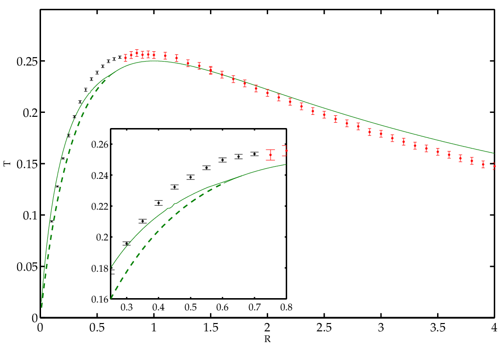
Altogether, a rather good agreement is obtained between mean-field and numerical results, though some systematic deviations appear, as seen on Fig. 6. These deviations might be due to underevaluated finite size effects (the number of agents used in the simulation is $N_{a}\sim 500$), but it is more likely to result from the simplifying assumptions made in the derivation the mean-field equations. Note however that the ranges in which continuous and discontinuous transitions are observed numerically are rather well reproduced by the mean-field argument.

In the present model, each agent has to choose between two options, namely going to the first or the second store. Such a binary choice can be encoded into a ’spin’ variable $s_{i}$, equal to $1$ if agent $i$ chooses the first shop, and to $-1$ in the opposite case. Though somehow artificial, this definition has the advantage that the order parameter $m$ introduced in Sec. 3.3 can be reexpressed as $m=N_{a}^{-1}\sum_{i}s_{i}$. This naturally suggests that the present model may exhibit, to some extend, an analogy to the Ising model. This analogy can be made more precise, at the mean-field level, in the following way. Let us modify the model in such a way that the freshness of products (which drives the evolution of the satisfaction of agents) is replaced by the opposite of the energy $E_{\mathrm{Ising}}$ of the mean-field Ising model, with $E_{\mathrm{Ising}}=-\frac{1}{2}N_{a}Jm^{2}$ ¹¹ 1 Strictly speaking, the magnetization $m$ should be computed from the last choice of the $N_{a}-1$ other agents.. Then the mean satisfaction $\sigma$ introduced in Sec. 3 evolves according to

$$\sigma(t+\tau_{0})=\alpha\sigma(t)-(1-\alpha)\Delta E,$$

(25)

with

$$\Delta E=-\frac{1}{2}N_{a}J\left[\left(m+\frac{1}{N_{a}}\right)^{2}-\left(m-\frac{1}{N_{a}}\right)^{2}\right]=-2Jm.$$

(26)

Note that the last equality has been obtained in the large $N_{a}$ limit. We then get the evolution equation, in the large memory limit $1-\alpha\ll 1$,

$$\frac{d\sigma}{dt}=\gamma[-\sigma+2Jm],$$

(27)

which is the analog of Eq. (6), with here again $\gamma=(1-\alpha)/\tau_{0}$. It is easy to check, using relation (7) to eliminate the variable $\sigma$, that the time evolution equation for $m$ is given by

$$\frac{dm}{dt}=\frac{\gamma}{T}(1-m^{2})\left[\frac{T}{2}\ln\left(\frac{1-m}{1+m}\right)+Jm\right].$$

(28)

Similarly to Eq. (17), the term between brackets can be written as the opposite of the derivative of a free energy $f(m)$,

$$f(m)=\frac{T}{2}(1+m)\ln(1+m)+\frac{T}{2}(1-m)\ln(1-m)-\frac{1}{2}Jm^{2}$$

(29)

which is, up to an additive constant $T\ln 2$, nothing but the standard mean-field free energy of the Ising model.

However, beyond mean-field, it is clear that the relation to the Ising model is at most an analogy. Indeed, the fact that the interaction between agents is here mediated by the ageing of products in each store rather than by an internal energy function makes the present model quite different from standard equilibrium models.

In this paper, we have studied a simple model of competing shops selling fresh products, retaining as main ingredients the ageing of products and the satisfaction of customers with respect to the freshness of products –considered to be the main factor influencing choices made by customers. Under these very simplifying assumptions, we found a surprisingly rich dynamics, with both continuous and discontinuous transitions between symmetric and symmetry-broken states. The overall agreement between numerical simulations and mean-field predictions was found to be satisfactory.

Several extensions could be interesting to study. For instance, other functional forms could be considered for the ageing function $h(\tau)$ introduced in Eq. (1), like

$$h(\tau)=\left(1-\frac{\tau}{\tau_{1}}\right)\,\theta\left(1-\frac{\tau}{\tau_{1}}\right)$$

(30)

where $\theta(x)$ is the Heaviside function. Such a form would be rather natural for products that can be sold only up to an expiration date. We have checked that the form (30) preserves the qualitative behaviour of the model. Another natural extension of this work would be to include more than two shops. Although we did not study this case in detail, a simple argument can already be given here. With a fixed overall number of agents $N_{a}$, adding shops reduces the nominal number of customers for a given shop. As a first approximation, a model with more than two shops can be described as a two-shop model with an effective number of agents $N_{a}^{\mathrm{eff}}<N_{a}$, resulting in an effective parameter $R^{\mathrm{eff}}>R$. If one starts from a low value of $R$ corresponding to the symmetric region, increasing the number of shops would then eventually lead to a value $R^{\mathrm{eff}}$ in the symmetry broken phase. It is thus likely that, for a given total number of agents, there is a maximal number of shops that can maintain a good level of activity, which seems to be consistent with conventional wisdom.

Further possible extensions may include taking into account explicitly the prices of products, as well as the costs associated to the shops (e.g., rent or salaries). In this context, one can imagine to include, in a simplified way, a dynamics of the shopkeeper who could modify the prices, or diversify the products, as a function of the dynamical state of the store. One might guess that such a dynamics could contribute to stabilize the symmetric states.

References

- [1] L. E. Reichl, A Modern Course in Statistical Physics, 2nd ed. (J. Wiley and Sons, New York, 1998).
- [2] K. Huang, Introduction to Statistical Physics, 2nd ed. (Taylor and Francis, London, 2001).
- [3] T. C. Schelling, Micromotives and Macrobehavior (Norton, New-York, 1978).
- [4] J. Toner, Y. Tu and S. Ramaswamy, Ann. Phys. 318, 170 (2005).
- [5] C. Castellano, S. Fortunato and V. Loreto, Rev. Mod. Phys. 81, 591 (2009).
- [6] D. L. Ryan, B. von Hohenbalken, D. S. West, Regional Science and Urban Economics 20, 313 (1990).
- [7] R. E. Krider and C. B. Weinberg, Journal of Retailing and Consumer Services 7, 1 (2000).
- [8] A. Bhatnagar and B. T. Ratchford, Intern. J. of Research in Marketing 21, 39 (2004).
- [9] M. C. W. Janssen, V. A. Karamychev, P. van Reeven, Regional Science and Urban Economics 35, 700 (2005).
- [10] H. Larralde, J. Stehlé, P. Jensen, Regional Science and Urban Economics 39, 343 (2009).
- [11] P. Jensen, Phys. Rev. E 74, 035101(R) (2006).
- [12] S. P. Anderson, A. De Palma, and J. F. Thisse, Discrete Choice Theory of Product Differentiation (MIT Press, Cambridge, MA, 1992).
- [13] V. Aguirregabiria and P. Mira, Journal of Econometrics 156, 38 (2010).
- [14] E. W. McLaughlin, Preventive Medicine 39, S81 (2004).
- [15] M. Tsiros and C. M. Heilman, Journal of Marketing 69, 114 (2005).
- [16] S. Grauwin, E. Bertin, R. Lemoy, and P. Jensen, Proc. Natl. Acad. Sci. USA 106, 20622 (2009).
- [17] K. Binder, “Monte-Carlo investigations of phase transitions and critical phenomena”, in Phase Transitions and Critical Phenomena, C. Domb and M. S. Green Eds, vol. 5b (New York, Academic Press, 1976).