Power density spectrum of nonstationary short–lived light curves
Abstract
The power density spectrum of a light curve is often calculated as the average of a number of spectra derived on individual time intervals the light curve is divided into. This procedure implicitly assumes that each time interval is a different sample function of the same stochastic ergodic process. While this assumption can be applied to many astrophysical sources, there remains a class of transient, highly nonstationary and short–lived events, such as gamma–ray bursts, for which this approach is often inadequate. The power spectrum statistics of a constant signal affected by statistical (Poisson) noise is known to be a in the Leahy normalisation. However, this is no more the case when a nonstationary signal is also present. As a consequence, the uncertainties on the power spectrum cannot be calculated based on the properties, as assumed by tools such as XRONOS powspec. We generalise the result in the case of a nonstationary signal affected by uncorrelated white noise and show that the new distribution is a non-central , whose non-central value is the power spectrum of the deterministic function describing the nonstationary signal. Finally, we test these results in the case of synthetic curves of gamma–ray bursts. We end up with a new formula for calculating the power spectrum uncertainties. This is crucial in the case of nonstationary short–lived processes affected by uncorrelated statistical noise, for which ensemble averaging does not make any physical sense.
Keywords:
methods: statistical — gamma-rays: bursts1 Introduction
The study of the temporal variability of time series in various branches of science and engineering has propelled the development of several techniques, both in frequency and time domains. Variability studies in the case of astronomical sources are crucial to gain insight over the dynamical and microphysical timescales, and therefore on the size of the emitting region as well as the nature itself of the emission process. This is of key importance in the X– and –ray domain, where remarkable flux variations are observed over timescales from days to ms.
Fourier techniques are widely used in this field, as witnessed by the popular timing analysis package xronos11 1 Available at http://heasarc.gsfc.nasa.gov/docs/xanadu/xronos/xronos.html. (Stella & Angelini, 1992) included in the NASA heasoft package22 2 Available at http://heasarc.gsfc.nasa.gov/docs/software/lheasoft/.. The Fourier spectral analysis is fundamental in the study of stationary processes, since it provides an immediate physical interpretation as a power-frequency distribution. The Fourier power density spectrum (hereafter, PDS) in particular decomposes the total variance of a given time series to the different frequencies thanks to Parseval’s theorem (e.g., van der Klis 1988; hereafter, K88). PDS analysis and related tools are suitable to both searching for possible periodic signals hidden in the data, and to characterising the so-called “red noise” connected with the presence of aperiodic variability.
Practically, in the most general case one divides the time series in multiple adjacent intervals, over which the corresponding PDS is calculated. Finally, for each frequency bin the resulting PDS value and uncertainty are the mean and standard deviation of the corresponding power distribution, as is routinely done by the dedicated xronos tool powspec (Stella & Angelini, 1992). However, the fundamental assumption behind this procedure is that each time interval represents a different sampling of the same stochastic stationary process. The operation of replacing ensemble averages with time averages of a single realisation makes sense only if the process is ergodic (e.g., Priestley 1981).
Astronomical X–ray data rely on photon counting instruments. As such, measurement uncertainties are often dominated by the photon counting statistics, i.e. the Poisson distribution. This translates into white noise in the PDS; adopting the normalisation introduced by Leahy et al. (1983) (hereafter L83), the power is known to follow a distribution with 2 degrees of freedom ().
When additional, genuine variability of the source is also present, the resulting power distribution changes correspondingly. For instance, there is a class of X–ray sources, such as Cyg X–1, whose time series are the result of a process characterised by source–intrinsic correlated noise, for which time averages of PDSs from individual intervals are still meaningful. These time series belong to a class of random processes whose PDS is still compatible with a rescaled distribution (K88; Israel & Stella 1996).
In the case of highly nonstationary and short–lived events such as gamma–ray bursts (GRBs), the problem of a proper treatment of the Fourier PDS requires particular care. Dividing the light curve of a single GRB into several sub–intervals, and deriving an average PDS does not make any physical sense, given that the phenomenon is everything but stationary. Therefore, only a single sample PDS can be calculated over the entire observation duration. In these cases the statistical distribution of the PDS remains to be determined in the more general case of red deterministic variability due to the source. One has then to be careful with assuming the 100% uncertainties on the PDS provided by standard tools such as powspec: indeed, this relies on the distribution, which does not hold any more in the more general case of a variable source with red noise.
In the GRB literature, there have been different approaches. In one case, if one considers a set of different time series due to different GRBs as many realisations of the same stochastic process, then averaging the PDS of different GRBs still make sense. However, it must be pointed out that a strong assumption lies behind this: i.e., there is a unique stochastic process giving rise to the variety of observed GRB time profiles. This way one gains insight into the properties of this general process, whose PDS is found to be described with a power–law, PDS (Beloborodov et al., 2000; Spada et al., 2000). In the other case, each GRB time profile is considered individually as the unique sample of a unique stochastic process, which is different from other GRBs. The statistics of its unique PDS is not known and is no more a . Monte Carlo simulations aimed at estimating the PDS uncertainties by generating other (synthetic) samples of the same process cannot make use of the observed sample curve (e.g., Ukwatta et al. 2011). Indeed, such a procedure increases the noise variance and changes the nature itself of the power distribution.
In this work we address the issue of a correct evaluation of the statistics of the PDS, and in particular of the power uncertainties, for a single sample of a nonstationary and short–lived signal, such as that of GRB time profiles. In this work time series are meant to be deterministic profiles affected by uncorrelated noise. We derived a formula for the variance of the PDS and show that it agrees with the known results of L83 in the pure white noise case. Finally, we test the validity of our results in the case of synthetic light curves of typical GRBs.
Hereafter, time series are assumed to be discrete, equispaced, and with no data gaps. Our treatment assumes the noise to be purely statistical and uncorrelated, and we consider the two cases of Poisson or Gaussian statistics, suitable to photon counting detectors. PDSs are calculated assuming the Leahy normalisation (L83). We therefore neglect dead time effects, which are known to affect the statistics and suppress the variance of the resulting time series (e.g., Müller 1973, K88).
2 Description
Let () be a time series observed within a time window with a duration . The corresponding bin times are . The observed series represents a sample function of the true time series we would have observed in the absence of statistical noise (e.g., with an infinite collecting area detector). Hereafter, random variables are written in bold. Each is therefore a single sample of the random variable , whose expected value and variance are defined as , and . The random variables are assumed to be independent, ().
The discrete Fourier transform (DFT) amplitudes are defined by
| (1) | |||||
| (2) |
where the corresponding -th frequency is . The highest frequency is the Nyquist frequency, . In the Leahy normalisation the power spectrum is defined by
| (3) |
or, equivalently,
| (4) |
, is the expected total variance. As shown in Section B, this happens to coincide with the total number of counts in the specific case of Poisson statistics, which explains the reason for the choice of this name. From equation (3) the expected value of the random variable is derived straightaway, and is
| (5) |
where we used . The first term in the right-hand side of equation (5) accounts for the statistical noise variance, also called “white” because it does not depend on frequency. When the signal is constant, (), is known to be distributed, except for the Nyquist frequency, for which is distributed and must be treated separately (L83). In the pure white noise case the second term vanishes, thus leaving .
In general, the second term can also be seen as the DFT of the autocorrelation function (ACF) defined by
| (6) |
assuming the periodic boundary condition . This is the discrete version of the Wiener–Khinchin theorem stating that the power spectrum of a time series is the Fourier transform of its ACF (e.g., Papoulis & Pillai 2002).
We define the power density spectrum of the deterministic function by
| (7) |
so that equation (5) can be written as
| (8) |
So far no assumption was made on the kind of the distribution of the random variables . Hereafter, we distinguish between the Gaussian and the Poisson noise cases.
2.1 Gaussian noise
Each random variable is distributed according to a normal . We can express equation (4) as the result of matrix products:
| (9) |
where is the column vector whose -th row element is , and is the element of . The matrix is a positive-definite quadratic form. As such, from the algebra of the quadratic forms (e.g., Ennis & Johnson 1993) the distribution of the random variable is a non-central if and only if the two following conditions are fulfilled:
where is the degrees of freedom, and
| (13) |
with being the column vector whose -th element is . Equation (13) follows from the definition of given in equation (7). is the covariance matrix, so its element is given by
| (14) |
where is Kronecker’s delta. To verify the first equation (2.1), we calculate the element of the matrix , which is found to be:
| (15) |
The second term of the right-hand side is identically zero when all the variances are equal. More generally, the second term of the right-hand side of equation (15) is O times . Therefore, equation (2.1) is approximately fulfilled in practical cases of interest.
The rank of does not depend on , so we can calculate it in the special case when (), i.e. the case of constant signal. We already know that is distributed (L83), so it must be .
This proves that in the more general case of a varying signal described by a deterministic function whose discrete values are given by (), and affected by pure uncorrelated Gaussian noise , the Leahy-normalised power spectrum distributes according to a non-central , where is (equation 13). The expected value of is already known from equation (5), while its variance is33 3 If is distributed, then , and Var.
| (16) |
Appendix A reports the direct calculation of Var and equation (35) reports the exact formula for the variance. In the case satisfies the conditions (2.1) with ,
| (17) |
where we used . Equations (16,17) can also be written as a function of the expected power:
Clearly, in the general case of uncorrelated noise and a significant power above the white noise level, i.e. when , assuming a 100% uncertainty on the resulting power spectrum , as assumed by widespread tools in X–ray astronomy such as XRONOS powspec overestimates the uncertainty. While the 100% uncertainty inherited from the distribution is correct under the assumption that all power is due to Poisson noise and intrinsic correlated noise, in the case of uncorrelated noise here considered from equation (2.1) the uncertainty is given by , and not . The two coincide only in the case of pure noise associated with a constant signal, so that . The 100% uncertainty assumed by XRONOS remains correct in the presence of genuine stochastic variability due to correlated noise.
In practice, when only a single sample series is available of a short–lived process, such as the time profile of a GRB, the deterministic series is not known a priori. However, one could constrain the probability density function (pdf) of , i.e. the unknown (equation 13), with the only sampled value . In principle, this makes no difference to taking the light curve with observed counts as instead of the unknown for a Poisson process (the Gaussian case is formally the same). We estimate , the best value for , adopting a Bayesian approach:
| (21) |
where is the posterior function of the parameters ( is fixed to either 1 or 2 depending on whether it is or not ) given the observed . The likelihood function is merely the pdf of , i.e. . The prior may include the knowledge one might have on prior to measuring , e.g. when a specific shape of the deterministic PDS is expected. In the most general case, we assume a uniform prior. The term normalises the likelihood function. For a given is chosen so as to maximise the posterior probability. In this case our approach is equivalent to a maximum likelihood estimation (MLE). In Appendix C we show that it is (), and that rapidly converges to () and to () for . We conservatively assumed ( for ) for all values of , to avoid the risk of underestimating the variance. Therefore, for a single time series consisting of an unknown deterministic function affected by uncorrelated white noise equations (16) and (17) are approximated to
Interestingly, the case of a constant variance (all are equal), for which the first equation (2.1) is fulfilled exactly (see equation 15), was discussed by Groth (1975). Apart from a scale factor of 2 in the definition of power, the probability density function he derived is precisely that of a non-central chi square with degrees of freedom, and a non-central parameter given by the deterministic (or “signal”, as he called it) power (see equations 12 and 14 therein). His treatment considered the case where the power is the sum of terms due to as many frequency bins, while here we consider the case.
2.2 Poisson noise
Each random variable is distributed according to a Poisson distribution with expected value . Since are no more normal, we cannot exploit the properties expressed by the conditions (2.1) for the Gaussian case. In Appendix B we calculate the corresponding variance of . Equation (43) reports the exact formula for Var.
The main results are the following:
- •
if the observed counts are so high as to ensure the Gaussian regime () the results are the same as those discussed in Section 2.1, since the overall process essentially becomes Gaussian.
- •
- •
3 Applications: gamma–ray burst light curves
We produced a number of GRB synthetic light curves to test the validity limits of the results we derived for nature of the the power spectrum distribution and summarised by equations (16–2.1). GRBs are particularly suitable to this aim, given their nature of highly nonstationary and short–lived phenomena. We adopted the fast-rise exponential decay (FRED) profile as modelled by Norris et al. (1996). This function satisfactorily describes the temporal behaviour of the simplest example of GRB light curve, which consists of a single pulse modelled as
where is the peak time, and are the rise and decay times, respectively, is the normalisation and is the peakedness (when the profile is a simple exponential, when it is a Gaussian). For a typical FRED it is , with an average value of – (Norris et al., 1996). The continuous power density spectrum of a FRED with (double exponential) can be calculated analytically, and apart from a normalisation term is found to be
| (28) |
Several examples of power spectra obtained for the more general case of a FRED with are discussed by Lazzati (2002).


We started with a FRED with the following parameters: s, s, , counts bin-1, s, superposed to a constant detector background with an average intensity of 1000 counts bin-1. We generated samples of this pulse with a bin time of ms, assuming Poisson statistics. The total number of bins amounts to 4096 (). Given the large number of counts per bin, this is equivalent to the Gaussian case. Figure 1 displays the synthetic curve of the deterministic model as well as one out of the simulated samples. The deterministic PDS is used for comparison to assess the goodness of the PDS of the sample curve, in particular of the uncertainties derived for the power adopting equation (2.1) as a function of frequency. This is shown by the ratio between the calculated and the scatter of the power of the synthetic PDSs observed for each corresponding frequency bin (bottom right panel of Fig. 1). Apparently, the ratio ranges between and . An overall comparison with the analogous ratio between the uncertainty provided by powspec and the corresponding value determined from the MC simulations (mid right panel of Fig 1) shows that the improvement is noteworthy. Furthermore, the accuracy of equation (2.1) is evident when the PDS is dominated by the deterministic power of the signal (at low frequencies). At high frequencies, where the white statistical noise dominates, the power uncertainty is systematically overestimated up to a factor of 2. However, compared to the values provided by powspec often underestimated by up to an order of magnitude, it still represents a significant improvement, particularly in the more conservative direction of overestimating rather than underestimating uncertainties.
So far this proves that equation (2.1) overall provides a satisfactory means for estimating the uncertainty on the PDS of a sample curve. We go further and test whether the distribution of the individual is indeed a non-central chi-square distribution. To this aim, from the PDS of the sample curve considered above we chose two frequencies and derived the corresponding power distribution from the synthetic PDSs. The result is displayed in Fig. 2. The expected non-central parameter for the corresponding was calculated with equations (7, 16).
Figure 3 shows the same FRED pulse 200 times fainter superposed to a correspondingly fainter constant background of 5 counts bin-1. The single variables cannot be approximately assumed to be normally distributed, so that we may test the Poisson regime. Still, the total number of counts is still very large, . This means that the results obtained for the Gaussian case should still hold. Indeed, both the comparison between the calculated uncertainties and the scatter of the corresponding power from the simulated PDSs gives similar results to the previous case (bottom right panel of Fig. 3). Likewise, the power distributions of individual frequency bins are fully compatible with the corresponding expected non-central chi-squares, as shown by Fig. 4.


4 Summary and Conclusions
We investigated the nature of the statistical distribution of the power density spectrum of a single, nonstationary, and short–lived time profile on a theoretical ground. This treatment assumes the time series to be deterministic profiles affected by uncorrelated noise. In other words, the time series here considered consist of a set of statistically independent, Poisson and normally distributed random variables, whose expected values represent the deterministic function of the varying signal to be studied.
We demonstrated that the probability density function of the power is a non-central , whose non-central parameter corresponds to the power of the deterministic function. This holds in the Gaussian case, as well as in the Poisson case, provided that the Gaussian limit of is fulfilled ( being the total number of counts). As a consequence, we provided a new formula for calculating the correct uncertainty of the power at each frequency as a function of the observed power itself. We finally showed the agreement with simulated light curves of typical GRB time profiles. These results provide a statistically solid basis to a proper treatment of power density spectra in the case of nonstationary and short–lived time series affected by uncorrelated noise.
Acknowledgments
The author is grateful to Mauro Orlandini and Raffaella Margutti for reading the manuscript and for their useful comments. The author also wishes to thank the referee Michiel van der Klis for the very useful comments. The author acknowledges ASI for financial support (ASI-INAF contract I/088/06/0).
Appendix A Variance of the power (Gaussian case)
The central moments of a random variable normally distributed as are
| (29) |
where the different variables at different values of are meant to be independent, so , . They can be used to calculate the corresponding noncentral moments through the following,
| (30) |
The noncentral moments are given by
| (31) |
The variance of is calculated directly from equation (3):
| (32) | |||||
where we used the definition of . The terms of equation (32) must conveniently be separated based on the different kind of moments. To simplify the notation, we define .
| (33) | |||||
We adopted the following notation: is a sum over , and , and is meant to exclude all the equality cases (, , ). Replacing the values of the corresponding moments,
| (34) | |||||
After a few passages, by adding and subtracting the terms excluded in the sums in equation (34), one ends up with the following:
| (35) | |||||
Equation (35) is exact. For the Nyquist frequency, equation (35) becomes
| (36) |
in agreement with equation (17). For the second term in the right-hand side of equation (35) is identically zero when all (), and it can be neglected when the ’s are comparable with each other, being O times the first term. Equation (35) can be approximated by
Appendix B Variance of the power (Poisson case)
The case of a process affected by Poisson noise is a more general case than that of a Gaussian noise, since the latter corresponds to the former in the high count rate regime, i.e. when it is . For a Poisson process, the central moments are
| (40) |
From equation (30) the corresponding noncentral moments are
| (41) |
In the Poisson case the normalisation constant is the expected total counts. The definition of the power spectrum is the same as that of equation (3). Using the first two moments of equation (41), calculating the expected value of is straightforward, and is found to be the same as equation (5).
Calculating the variance of in the Poisson case is formally the same as the Gaussian case up to equation (33), i.e., prior to substituting the specific values of the moments. At this point the two cases must be treated separately. Replacing the moments of equation (41) in (33), and defining as before, it becomes
| (42) | |||||
Similarly to what was done in section A, adding and subtracting the excluded terms in the sums, after a few passages one ends up with
| (43) | |||||
As done for the Gaussian case, we have to treat the Nyquist frequency separately. When , equation (43) becomes
| (44) |
which is equivalent to equation (36) in the limit. In the special case of a constant signal (), equation (43) reduces to
in agreement with the results of L83. In the more general case of a nonstationary signal , in the limit , equation (43) can be approximated by
| (48) | |||||
Not surprisingly, equation (48) is the same as (35) upon replacing with , as expected for a Poisson variable in the Gaussian limit. As discussed in Appendix A, the result in equation (48) can be approximated by equation (A), provided that . When the Gaussian limit is not satisfied, i.e., when is just a few, we note that the relation between expected value and variance for a noncentral chi-square distributed random variable with degrees of freedom is not fulfilled:
| (49) | |||||
| (50) | |||||
We conclude that for few, the distribution of the power spectrum at a given frequency is not a noncentral , as found in the Gaussian limit, and the expression for the variance to be used is given by equation (50). In the same regime of few, also deviates from a noncentral distribution, given that equation (44) does not fulfil any more the corresponding relation between expected value and variance. The exact formula for the variance of the Nyquist frequency power therefore remains equation (44).
Appendix C Maximum likelihood estimation
The and cases must be treated separately, given that the probability density functions of the corresponding random variables are non-central chi squares with and degrees of freedom, respectively. The purpose is to find the value for the non-central parameter which maximises the likelihood function for a given measured value .
First, let us consider the case, for which it is . It is
| (51) |
When equation (51) reduces to a simple exponential, so that . For , it is . For , is found by requiring
| (52) |
equivalent to
| (53) |
where is the modified Bessel function of the first kind and index . At the solution is . Numerical solutions to equation 53 are displayed in Figure 5 (solid line), which shows how rapidly converges to as a function of .
In the case it is and the interested random variable is . To simplify the notation, let us define , so it is
| (54) |
When equation (54) monotonically decreases for , so it is . When , the maximum is found analogously to equation (52), thus
| (55) |
equivalent to
| (56) |
Analogously to the case, the solution is and rapidly converges to , as shown in Figure 5 (dashed line).
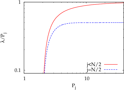
Summing up, in both cases it is for , and for it asymptotically tends to () for ().
References
- Beloborodov et al. (2000) Beloborodov A. M., Stern B. E., Svensson R., 2000, ApJ, 535, 158
- Ennis & Johnson (1993) Ennis D. M., Johnson N. L., 1993, Comm. Statist., 22, 897
- Groth (1975) Groth E. J., 1975, ApJS, 29, 285
- Israel & Stella (1996) Israel G. L., Stella L., 1996, ApJ, 468, 369
- Lazzati (2002) Lazzati D., 2002, MNRAS, 337, 1426
- Leahy et al. (1983) Leahy D. A., Darbro W., Elsner R. F., Weisskopf M. C., Sutherland P. G., Kahn S., Grindlay J. E., 1983, ApJ, 266, 160 (L83)
- Müller (1973) Müller J. W., 1973, Nuc. Instr. and Meth., 112, 47
- Norris et al. (1996) Norris J. P., Nemiroff R. J., Bonnell J. T., Scargle J. D., Kouveliotou C., Paciesas W. S., Meegan C. A., Fishman G. J., 1996, ApJ, 459, 393
- Papoulis & Pillai (2002) Papoulis A., S. U. Pillai, 2002, Probability, Random Variables and Stochastic Processes. Fourth Edition. McGraw Hill, New York, NY
- Priestley (1981) Priestley M. B., 1981, Spectral Analysis and Time Series. Academic Press, London, UK
- Spada et al. (2000) Spada M., Panaitescu A., Mészáros P., 2000, ApJ, 537, 824
- Stella & Angelini (1992) Stella L., Angelini A., 1992, in Di Gesù, L. Scarsi, R. Buccheri, P. Crane, M. C. Maccarone, H. V. Zimmerman, eds, Data Analysis in Astronomy IV. Plenum, New York, p. 59
- Ukwatta et al. (2011) Ukwatta T., et al., 2011, MNRAS, 412, 875
- van der Klis (1988) van der Klis M., 1988, in Ögelman H., van den Heuvel E. P. J., eds, Timing Neutron Stars. NATO ASI, Series C, Kluwer, Dordrecht, p. 27 (K88)