On Multilinear Principal Component Analysis of Order-Two Tensors

Hung Hung Affiliation: Institute of Epidemiology and Preventive Medicine, National Taiwan University Pei-Shien Wu Affiliation: Department of Mathematics, National Taiwan University I-Ping Tu Note: Corresponding author. Email address: iping@stat.sinica.edu.tw Affiliation: Institute of Statistical Science, Academia Sinica Su-Yun Huang Affiliation: Institute of Statistical Science, Academia Sinica

Abstract

Principal Component Analysis (PCA) is a commonly used tool for dimension reduction in analyzing high dimensional data; Multilinear Principal Component Analysis (MPCA) has the potential to serve the similar function for analyzing tensor structure data. MPCA and other tensor decomposition methods have been proved effective to reduce the dimensions for both real data analyses and simulation studies (Ye, 2005; Lu, Plataniotis and Venetsanopoulos, 2008; Kolda and Bader, 2009; Li, Kim and Altman, 2010). In this paper, we investigate MPCA’s statistical properties and provide explanations for its advantages. Conventional PCA, vectorizing the tensor data, may lead to inefficient and unstable prediction due to its extremely large dimensionality. On the other hand, MPCA, trying to preserve the data structure, searches for low-dimensional multilinear projections and decreases the dimensionality efficiently. The asymptotic theories for order-two MPCA, including asymptotic distributions for principal components, associated projections and the explained variance, are developed. Finally, MPCA is shown to improve conventional PCA on analyzing the Olivetti Faces data set, by constructing more module oriented basis in reconstructing the test faces.

Keywords and phrases: Asymptotic theory, Dimension reduction, Image reconstruction, Multilinear principal component analysis, Principal component analysis, Tensor.

1 Introduction

Dimension reduction is a key step for high dimensional data analysis. Principal component analysis (PCA) is probably the most commonly used method for dimension reduction. Given $n$ observations on $m$ variables, PCA calculates the $m\times m$ covariance matrix and solves the eigenvalue decomposition problem for the covariance matrix. The goal is to choose a smaller set of eigenvectors as a new coordinate system so that the newly transformed variables can retain the most data variation. This PCA approach has been widely applied in many scientific fields for dimension reduction and compact data representation (Jolliffe, 2002), where the collected data are organized in an $n\times m$ design matrix with each row representing an observation and each column a variable.

When data are tensor objects, traditional analysis vectorizes each of the tensor objects into a long vector and arranges these vectorized objects in a design matrix form. Subsequent analysis is followed in the usual way. Nevertheless, this approach usually produces a large number of variables, where the available sample size is relatively small, and many existing statistical methods fail to apply. For a typical example, like the Olivetti Faces data set to be used in an experimental study later, there are 400 images each with $64\times 64$ pixels. Vectorizing each image leads to a design matrix of size $400\times 4096$ , which the variable dimension $m$ largely exceeds the sample size $n$ .

One strategy to overcome this difficulty is to take advantage of the natural tensor structure of the data. Singular value decomposition (SVD) is an example. Given a $p\times q$ matrix $X$ which can be treated as an order-two tensor, SVD can decompose two directional spaces simultaneously: $X=USV^{T}=\sum_{i=1}^{p\wedge q}s_{i}u_{i}v_{i}^{T}$ , where $U=[u_{1},...,u_{p}]\in\mathfrak{R}^{p\times p}$ and $V=[v_{1},...,v_{q}]\in\mathfrak{R}^{q\times q}$ are, respectively, the left and right singular vectors, $S$ is a diagonal matrix of size $p\times q$ with diagonal elements $\{s_{1},...,s_{(p\wedge q)}\}$ . The dimension can be reduced when the index $i$ is properly truncated. De Lathauwer, De Moor and Vandewalle (2000a) then generalized the SVD to high-order SVD (HOSVD) for a given $N^{\rm th}$ -order tensor object $A\in\Re^{I_{1}\times\cdots\times I_{N}}$ . Further, they formulated the problem of “best rank- $(R_{1},\cdots,R_{N})$ approximation of higher-order tensors” in the least-squares sense, and discussed many algorithms to achieve this task (De Lathauwer, De Moor and Vandewalle, 2000b).

Later, Yang et al. (2004) proposed two-dimensional PCA (2DPCA) for analyzing image data, which are order-two tensors. An improved two-directional two-dimensional PCA ( ${\rm(2D)}^{2}$ PCA) was developed in Zhang and Zhou (2005), which was shown to perform better than 2DPCA through simulation studies. Ye (2005) formulated the problem of generalized low rank approximation of matrices, which can be treated as a sample extension of the best rank- $(R_{1},R_{2})$ approximation for order-two tensors in De Lathauwer, De Moor and Vandewalle (2000b). Lu, Plataniotis and Venetsanopoulos (2008) further generalized the work of Ye (2005) and proposed multilinear PCA (MPCA) for tensor objects of arbitrary orders. There are other tensor decomposition methods for dimension reduction. For instance, Kolda and Bader (2009) provided a general overview of current development of tensor decomposition methods for unsupervised learning, their applications, and available softwares; Li, Kim and Altman. (2010) considered the tensor decomposition methods for supervised learning such as regression and classification.

Similar to conventional PCA, the goal of MPCA is to look for low-dimensional multilinear projection for tensor objects that captures the most data variation. Back to the example of Olivetti Faces, one eigenvector in conventional PCA creates an image basis element that contains 4095 free parameters. By contrast, one image basis element in MPCA or (2D)²PCA, which involves the Kronecker product of a column vector and a row vector, contains 126 free parameters. From the viewpoint of the number of parameters required to specify one basis element, MPCA is expected to perform better than conventional PCA, when the sample size is small to moderate, like this Olivetti Faces example. Compared to (2D)²PCA, MPCA has the advantage of capturing more data variation by the chosen image basis, because of its specific criterion. MPCA has been successfully applied in real data analysis and checked by simulations (Ye, 2005; Lu et al., 2008). Yet, to our best knowledge, there is neither statistical justification nor asymptotic study for MPCA.

In this paper, we try to establish some relevant properties of order-two MPCA from a statistical point of view. Our study is based on the following model:

X=\mu+A_{0}UB_{0}^{T}+\varepsilon,

(1)

where $\mu\in\Re^{p\times q}$ is the mean parameter of $X$ , $A_{0}\in\Re^{p\times p_{0}}$ and $B_{0}\in\Re^{q\times q_{0}}$ with $p_{0}\leq p$ and $q_{0}\leq q$ are non-random basis matrices, $U\in\Re^{p_{0}\times q_{0}}$ is a random coordinate matrix with $E[U]=0$ and a strictly positive definite covariance matrix ${\rm Cov}({\sf vec}(U))=T\in\Re^{m_{0}\times m_{0}}$ , where $m_{0}=p_{0}q_{0}$ and ${\sf vec}(\cdot)$ is the operator that stacks the columns of a tensor into a long vector. The error term $\varepsilon\in\Re^{p\times q}$ is a random matrix independent of $U$ and with $E[\varepsilon]=0$ and ${\rm Cov}({\sf vec}(\varepsilon))=\sigma^{2}I_{m}$ , where $m=pq$ . Under model (1) which characterizes the tensor structure of $X$ , we justify the validity of MPCA. Asymptotic properties of MPCA are rigorously developed, including asymptotic distributions for principal components, associated projections and the explained variance. It is also shown that MPCA is asymptotically more efficient than (2D)²PCA in estimating the target dimension reduction subspace. Furthermore, a test of dimensionality is developed, based on the derived asymptotic results.

This paper is organized as follows. Section 2 presents some properties of the estimation for the target subspace and a test for its dimensionality. The relations between MPCA and both conventional PCA and (2D)²PCA are also discussed in this section. In section 3, the asymptotic theory of MPCA is developed. In section 4, the performance of MPCA and its comparison with conventional PCA is demonstrated by analyzing the Olivetti Faces data set. The paper ends with a brief discussion. Technical proofs of main results are deferred to the Appendix.

2 MPCA

MPCA, as a dimension reduction algorithm, is originally designed to search basis matrices $\{A,B\}$ and coordinate matrices $U_{i}$ ’s that best approximate the observed data $X_{i}$ as $AU_{i}B^{T}$ for $i=1,\dots,n$ . Although many simulation studies and real data analyses in literature support the usage of MPCA and multilinear tensor decomposition (Ye, 2005; Lu et al., 2008; Kolda and Bader, 2009; Li et al., 2010), there is no theoretical study from the statistical point of view. Let $\otimes$ be the Kronecker product. Then, there is an equivalent formula for model (1)

X=\mu+A_{0}UB_{0}^{T}+\varepsilon~~\Leftrightarrow~~{\sf vec}(X-\mu)=(B_{0}\otimes A_{0}){\sf vec}(U)+{\sf vec}(\varepsilon)

(2)

by the fact that ${\sf vec}(A_{0}UB_{0}^{T})=(B_{0}\otimes A_{0}){\sf vec}(U)$ . Without loss of generality, we may assume that $A_{0}$ and $B_{0}$ are orthogonal matrices, i.e., $A_{0}^{T}A_{0}=I_{p_{0}}$ and $B_{0}^{T}B_{0}=I_{q_{0}}$ . Model (1) thus ensures that, without considering the error term $\varepsilon$ , the columns and rows of $(X-\mu)$ belong to ${\rm span}(A_{0})$ and ${\rm span}(B_{0})$ , respectively, and ${\sf vec}(X-\mu)$ belongs to the subspace ${\rm span}(B_{0})\otimes{\rm span}(A_{0})={\rm span}(B_{0}\otimes A_{0})$ . It is then reasonable to estimate ${\rm span}(B_{0}\otimes A_{0})$ for follow-up analysis such as data compression, pattern recognition, regression analysis, etc. In this section, we show that, under model (1), MPCA actually attempts to extract a basis pair $\{A,B\}$ targeting the subspace ${\rm span}(B_{0}\otimes A_{0})$ . Proposition 2.2 below proves the existence of a solution pair $\{A,B\}$ . Proposition 2.5 summarizes that the inclusion relation between ${\rm span}(A)$ (resp., ${\rm span}(B)$ ) and the target dimension reduction subspace ${\rm span}(A_{0})$ (resp., ${\rm span}(B_{0})$ ), depends on the size comparison between the specified dimensionality ${\tilde{p}}$ (resp., ${\tilde{q}}$ ) and $p_{0}$ (resp., $q_{0}$ ). Recognizing the important roles of ${\tilde{p}}$ and ${\tilde{q}}$ , we construct a hypothesis test for choosing ${\tilde{p}}$ and ${\tilde{q}}$ . These works justify the usage of MPCA in extracting the relevant basis for subsequent analysis, provided the data has a natural tensor structure.

2.1 Estimation

Let $\{X_{i}\}_{i=1}^{n}$ be the collected data set which are assumed to be random copies of a random matrix $X\in\Re^{p\times q}$ . MPCA aims to extract the basis pair that best approximate $\{X_{i}\}_{i=1}^{n}$ while preserving the tensor structure of them. In particular, for a pre-specified dimensionality $({\tilde{p}},{\tilde{q}})$ , Ye (2005) proposed a criterion to find $A\in{\cal O}_{p,{\tilde{p}}},B\in{\cal O}_{q,{\tilde{q}}}$ , and $\{U_{i}\}_{i=1}^{n}$ that minimize

\frac{1}{n}\sum_{i=1}^{n}\|(X_{i}-\bar{X})-AU_{i}B^{T}\|_{F}^{2},

(3)

where $\bar{X}=\frac{1}{n}\sum_{i=1}^{n}X_{i}$ is the sample mean matrix, $\|\cdot\|_{F}$ is the Frobenius norm of a matrix, and ${\cal O}_{\ell,\tilde{\ell}}$ is the collection of all orthogonal matrices $M$ of size $\ell\times\tilde{\ell}$ such that $M^{T}M=I_{\tilde{\ell}}$ . Note that the objective function (3) can be expressed as

\frac{1}{n}\sum_{i=1}^{n}\|{\sf vec}(X_{i}-{\bar{X}})-(B\otimes A){\sf vec}(U_{i})\|^{2}_{2}.

(4)

If we replace $(B\otimes A)$ by $\Gamma$ in (4), the minimization problem then becomes the conventional PCA. From this viewpoint, MPCA can be treated as a constrained PCA with the tensor constraint $\Gamma=(B\otimes A)$ , where $A\in{\cal O}_{p,{\tilde{p}}}$ and $B\in{\cal O}_{q,{\tilde{q}}}$ . The following theorem established in Ye (2005) characterizes some useful properties of the solutions of the minimization problem (3). In the rest of discussion, $P_{M}$ denotes the orthogonal projection matrix onto ${\rm span}(M)$ and $Q_{M}=I-P_{M}$ .

Theorem 2.1.

(Ye, 2005) Let $\widehat{A},\widehat{B},\{\widehat{U}_{i}\}_{i=1}^{n}$ constitutes a minimizer for (3) under the dimensionality $({\tilde{p}},{\tilde{q}})$ . Then,

(a)

$\widehat{U}_{i}=\widehat{A}^{T}(X_{i}-{\bar{X}})\widehat{B}$ .
(b)

$\{\widehat{A},\widehat{B}\}$ is the maximizer of $\frac{1}{n}\sum_{i=1}^{n}\|A^{T}(X_{i}-{\bar{X}})B\|_{F}^{2}$ .
(c)

$\widehat{A}$ consists of the leading ${\tilde{p}}$ eigenvectors of $\frac{1}{n}\sum_{i=1}^{n}(X_{i}-{\bar{X}})P_{\widehat{B}}(X_{i}-{\bar{X}})^{T}$ , and $\widehat{B}$ consists of the leading ${\tilde{q}}$ eigenvectors of $\frac{1}{n}\sum_{i=1}^{n}(X_{i}-{\bar{X}})^{T}P_{\widehat{A}}(X_{i}-{\bar{X}})$ .

Similarly, we can define a population version of (3): $E\|(X-\mu)-AUB^{T}\|_{F}^{2}$ , and the corresponding minimizer should follow Theorem 2.1 such that the minimizer over $A\in{\cal O}_{p,{\tilde{p}}}$ and $B\in{\cal O}_{q,{\tilde{q}}}$ , is equivalent to the maximizer of the maximization problem:

\mathop{\rm argmax}_{A\in{\cal O}_{p,{\tilde{p}}},B\in{\cal O}_{q,{\tilde{q}}}}E\|A^{T}(X-\mu)B\|_{F}^{2}=\mathop{\rm argmax}_{A\in{\cal O}_{p,{\tilde{p}}},B\in{\cal O}_{q,{\tilde{q}}}}{\rm trace}\left\{(B\otimes A)^{T}\Sigma(B\otimes A)\right\},

(5)

where $\Sigma={\rm Cov}({\sf vec}(X))$ . The following proposition gives the existence of the solution.

Proposition 2.2.

For a fixed but arbitrary positive semi-definite matrix $\Sigma$ of size $pq\times pq$ , solution(s) to the maximization problem (5) exists.

Note that we do not need the model assumption (1) for Proposition 2.2. Also note that Proposition 2.2 applies to problem (3) as well by replacing $\Sigma$ with its sample estimate $S_{n}$ , the sample covariance matrix of $\{{\sf vec}(X_{i})\}_{i=1}^{n}$ , and by rephrasing the maximization problem into the equivalent minimization problem. With the existence of the maximizer in (5) we can formally define the tensor principal components and the MPCA subspace.

Definition 2.3.

For a pre-specified dimensionality $({\tilde{p}},{\tilde{q}})$ , let $\{A,B\}$ be the unique solution to the maximization problem (5), where $A$ and $B$ can be expressed in their columns as $A=[a_{1},\dots,a_{\tilde{p}}]$ and $B=[b_{1},\dots,b_{\tilde{q}}]$ . We call $\{b_{j}\otimes a_{i}:1\leq i\leq{\tilde{p}},1\leq j\leq{\tilde{q}}\}$ the tensor principal components, and ${\rm span}(B\otimes A)$ the MPCA subspace of dimensionality $({\tilde{p}},{\tilde{q}})$ .

Using similar arguments as in Theorem 2.1 (c), we have that $A$ and $B$ consist of the leading ${\tilde{p}}$ and ${\tilde{q}}$ eigenvectors of $E[(X-\mu)P_{B}(X-\mu)^{T}]$ and $E[(X-\mu)^{T}P_{A}(X-\mu)]$ , respectively. Since

	$\displaystyle E[(X-\mu)P_{B}(X-\mu)^{T}]=\sum_{j=1}^{{\tilde{q}}}E[(X-\mu)(b_{j}b_{j}^{T})(X-\mu)^{T}]=\sum_{j=1}^{{\tilde{q}}}(b_{j}\otimes I_{p})^{T}\Sigma(b_{j}\otimes I_{p}),$		(6)
	$\displaystyle E[(X-\mu)^{T}P_{A}(X-\mu)]=\sum_{i=1}^{{\tilde{p}}}E[(X-\mu)^{T}(a_{i}a_{i}^{T})(X-\mu)]=\sum_{i=1}^{{\tilde{p}}}(a_{i}\otimes I_{p})^{T}\Sigma(a_{i}\otimes I_{p}),$		(7)

equivalently, $\{A,B\}$ consist of the leading solutions of the system of stationary equations

	$\displaystyle\left(\sum_{j=1}^{{\tilde{q}}}(b_{j}\otimes I_{p})^{T}\Sigma(b_{j}\otimes I_{p})\right)a_{i}$	$\displaystyle=$	$\displaystyle\lambda_{i}a_{i},~i=1,\cdots,{\tilde{p}},$
	$\displaystyle\left(\sum_{i=1}^{{\tilde{p}}}(I_{q}\otimes a_{i})^{T}\Sigma(I_{q}\otimes a_{i})\right)b_{j}$	$\displaystyle=$	$\displaystyle\xi_{j}b_{j},~j=1,\cdots,{\tilde{q}},$

over $A\in\mathcal{O}_{p\times{\tilde{p}}}$ and $B\in\mathcal{O}_{q\times{\tilde{q}}}$ , where the ordering is determined by the corresponding eigenvalues $\lambda_{1}\geq\cdots\geq\lambda_{{\tilde{p}}}\geq 0$ and $\xi_{1}\geq\cdots\geq\xi_{{\tilde{q}}}\geq 0$ .

Remark 2.4.

Obviously $\lambda_{i}$ ’s, $a_{i}$ ’s, $\xi_{j}$ ’s and $b_{j}$ ’s depend on $\Sigma$ . Besides such dependence, they also depend on the dimensionality $({\tilde{p}},{\tilde{q}})$ . A more precise notation for them should be $\lambda_{i}(\Sigma,{\tilde{p}},{\tilde{q}})$ , $a_{i}(\Sigma,{\tilde{p}},{\tilde{q}})$ , $\xi_{j}(\Sigma,{\tilde{p}},{\tilde{q}})$ and $b_{j}(\Sigma,{\tilde{p}},{\tilde{q}})$ . However, for notation simplicity, we use $\lambda_{i}$ , $a_{i}$ , $\xi_{j}$ and $b_{j}$ , unless we want to emphasize on their dependence on $(\Sigma,{\tilde{p}},{\tilde{q}})$ .

From Remark 2.4, for any fixed $({\tilde{p}},{\tilde{q}})$ , we could define the sample analogues $\{\widehat{A},\widehat{B}\}$ , $\hat{\lambda}_{i}$ ’s, and $\hat{\xi}_{j}$ ’s by replacing $\Sigma$ with the sample covariance matrix $S_{n}$ . In the rest of the discussion, with pre-specified dimensionality $({\tilde{p}},{\tilde{q}})$ , we denote the solution of (5) by $\{A,B\}$ and the population tensor principal components by $(B\otimes A)$ , and the corresponding sample analogues by $\{{\widehat{A}},{\widehat{B}}\}$ and $({\widehat{B}}\otimes{\widehat{A}})$ . Finding principal components in conventional PCA is equivalent to an eigenvalue-problem. However, there is no explicit solution of $\{\widehat{A},\widehat{B}\}$ for MPCA; therefore, an algorithm was proposed. The GLRAM algorithm of Ye (2005) to obtain $\{\widehat{A},\widehat{B}\}$ is summarized below.

GLRAM (Ye, 2005): Given a random initial $A^{(0)}\in\mathcal{O}_{p\times{\tilde{p}}}$ . For $k=1,2,\cdots,$

1.

Obtain the maximizer $B^{(k+1)}=\arg\max_{B\in\mathcal{O}_{q\times{\tilde{q}}}}\frac{1}{n}\sum_{i=1}^{n}\|A^{(k)T}(X_{i}-\bar{X})B\|_{F}^{2}$ .
2.

Obtain the maximizer $A^{(k+1)}=\arg\max_{A\in\mathcal{O}_{p\times{\tilde{p}}}}\frac{1}{n}\sum_{i=1}^{n}\|A^{T}(X_{i}-\bar{X})B^{(k+1)}\|_{F}^{2}$ .
3.

Repeat Steps 1-2 until there is no significant difference between $\frac{1}{n}\sum_{i=1}^{n}\|A^{(k)T}(X_{i}-\bar{X})B^{(k)}\|_{F}^{2}$ and $\frac{1}{n}\sum_{i=1}^{n}\|A^{(k+1)T}(X_{i}-\bar{X})B^{(k+1)}\|_{F}^{2}$ . Output $\{\widehat{A},\widehat{B}\}=\{A^{(k+1)},B^{(k+1)}\}$ .

For any fixed $A^{(k)}$ or $B^{(k+1)}$ , the optimization problems in Steps 1 and 2 are the usual eigenvalue-problems of sizes $p$ and $q$ , respectively. Hence, $A^{(k+1)}$ and $B^{(k+1)}$ can be easily obtained. Moreover, the algorithm ensures the quantity $\frac{1}{n}\sum_{i=1}^{n}\|A^{(k)T}(X_{i}-\bar{X})B^{(k)}\|_{F}^{2}$ to be monotonically increasing as $k$ increases and, hence, the solution must exist since $\frac{1}{n}\sum_{i=1}^{n}\|A^{(k)T}(X_{i}-\bar{X})B^{(k)}\|_{F}^{2}$ is bounded above by $\frac{1}{n}\sum_{i=1}^{n}\|X_{i}-\bar{X}\|_{F}^{2}$ . Because GLRAM can only find a local maximum (depends on the chosen random initial $A^{(0)}$ ), multiple random initials are suggested by Ye (2005) to ensure the global maximum. In contrast to this suggestion, we propose to use the leading $\tilde{p}$ eigenvectors of $\frac{1}{n}\sum_{i=1}^{n}(X_{i}-\bar{X})(X_{i}-\bar{X})^{T}$ as an initial of $A^{(0)}$ .

We observe that hierarchical nesting structure may not exist for MPCA. Precisely, if $({\tilde{p}}^{\prime},{\tilde{q}}^{\prime})\leq({\tilde{p}},{\tilde{q}})$ with the corresponding solution pairs $\{\widehat{A}^{\prime},\widehat{B}^{\prime}\}$ and $\{\widehat{A},\widehat{B}\}$ , respectively, there is no guarantee that ${\rm span}(\widehat{A}^{\prime})\subseteq{\rm span}(\widehat{A})$ , nor ${\rm span}(\widehat{B}^{\prime})\subseteq{\rm span}(\widehat{B})$ . In the population level, however, there certainly exist relationships between the target subspaces and the MPCA subspaces prescribed by the optimization problem (5).

Proposition 2.5.

Assume model (1) and let $\{A,B\}$ be the solution pair to the maximization problem (5) under dimensionality $({\tilde{p}},{\tilde{q}})$ .

(a)

If ${\tilde{p}}\geq p_{0}$ and ${\tilde{q}}\geq q_{0}$ , then ${\rm span}(A)\supseteq{\rm span}(A_{0})$ and ${\rm span}(B)\supseteq{\rm span}(B_{0})$ .
(b)

If ${\tilde{p}}<p_{0}$ and ${\tilde{q}}\geq q_{0}$ , then ${\rm span}(A)\subsetneq{\rm span}(A_{0})$ and ${\rm span}(B)\supseteq{\rm span}(B_{0})$ .
(c)

If ${\tilde{p}}\geq p_{0}$ and ${\tilde{q}}<q_{0}$ , then ${\rm span}(A)\supseteq{\rm span}(A_{0})$ and ${\rm span}(B)\subsetneq{\rm span}(B_{0})$ .
(d)

If ${\tilde{p}}<p_{0}$ and ${\tilde{q}}<q_{0}$ , then ${\rm span}(A)\subsetneq{\rm span}(A_{0})$ and ${\rm span}(B)\subsetneq{\rm span}(B_{0})$ .

Even though there is no general hierarchical nesting structure for MPCA subspaces, Proposition 2.5 ensures the existence of a specific nesting structure, which the extracted MPCA subspace is a proper subspace of the target subspace if the dimension is under-specified, and contains the target subspace if the dimension is over-specified. It also implies that MPCA indeed searches the true target subspace ${\rm span}(B_{0}\otimes A_{0})$ when $({\tilde{p}},{\tilde{q}})=(p_{0},q_{0})$ is correctly specified. As a result, these arguments provide a justification of using ${\rm span}(\widehat{B}\otimes\widehat{A})$ in the sample level for subsequent statistical analysis.

2.2 Connection with ${\rm\textbf{(2D)}}^{2}$ PCA and conventional PCA

The ${\rm(2D)}^{2}$ PCA is another method to extract basis for tensor objects. For a given dimensionality $({\tilde{p}},{\tilde{q}})$ , the population ${\rm(2D)}^{2}$ PCA components $A^{*}=[a_{1}^{*},\cdots,a_{{\tilde{p}}}^{*}]$ and $B^{*}=[b_{1}^{*},\cdots,b_{{\tilde{q}}}^{*}]$ are defined to be the leading ${\tilde{p}}$ and ${\tilde{q}}$ eigenvectors of $E[(X-\mu)(X-\mu)^{T}]$ and $E[(X-\mu)^{T}(X-\mu)]$ with the corresponding eigenvalues $\{\lambda_{i}^{*}:1\leq i\leq{\tilde{p}}\}$ and $\{\xi_{j}^{*}:1\leq j\leq{\tilde{q}}\}$ . The sample analogues, denoted by $\widehat{A}^{*}$ , $\widehat{B}^{*}$ , $\hat{\lambda}_{i}^{*}$ , and $\hat{\xi}_{j}^{*}$ are similarly defined to be the leading eigenvectors and eigenvalues of $\frac{1}{n}\sum_{i=1}^{n}(X_{i}-\bar{X})(X_{i}-\bar{X})^{T}$ and $\frac{1}{n}\sum_{i=1}^{n}(X_{i}-\bar{X})^{T}(X_{i}-\bar{X})$ . The following proposition states a connection between the ${\rm(2D)}^{2}$ PCA and MPCA in the population level.

Proposition 2.6.

Assume model (1) and that $\{\lambda_{i}^{*}:1\leq i\leq p_{0}\}$ and $\{\xi_{j}^{*}:1\leq j\leq q_{0}\}$ are simple roots.

(a)

If $\,{\tilde{q}}\geq q_{0}$ , then MPCA and (2D)²PCA share the same leading $(p_{0}\wedge{\tilde{p}})$ eigenvectors, i.e., $a_{i}=a_{i}^{*}$ for $i=1,\cdots,(p_{0}\wedge{\tilde{p}})$ . Moreover, $\lambda_{i}^{*}-\lambda_{i}=(q-{\tilde{q}})\sigma^{2}$ for $i=1,\dots,{\tilde{p}}$ .
(b)

If $\,{\tilde{p}}\geq p_{0}$ , then MPCA and (2D)²PCA share the same leading $(q_{0}\wedge{\tilde{q}})$ eigenvectors, i.e., $b_{j}=b_{j}^{*}$ for $i=1,\cdots,(q_{0}\wedge{\tilde{q}})$ . Moreover, $\xi_{j}^{*}-\xi_{j}=(p-{\tilde{p}})\sigma^{2}$ for $j=1,\dots,{\tilde{q}}$ .

When the dimension $({\tilde{p}},{\tilde{q}})$ is adequate, Proposition 2.6 implies that ${\rm(2D)}^{2}$ PCA and MPCA, in the population level, actually target the same subspace ${\rm span}(B_{0}\otimes A_{0})$ under model (1). However, there is no guarantee that the extracted bases $\{\widehat{A}^{*},\widehat{B}^{*}\}$ of ${\rm(2D)}^{2}$ PCA also maximize the sample version of (5). Though, under the setting of Proposition 2.6, $E[(X-\mu)P_{B}(X-\mu)^{T}]$ and $E[(X-\mu)(X-\mu)^{T}]$ have the same leading eigenvectors, we expect an efficiency gain in using $E[(X-\mu)P_{B}(X-\mu)^{T}]$ , since it is less noise-contaminated than $E[(X-\mu)(X-\mu)^{T}]$ . A rigorous proof of efficiency gain is provided in Section 3.

Remark 2.7.

From Proposition 2.6, it is suggested to select $({\tilde{p}},{\tilde{q}})$ through ${\rm(2D)}^{2}$ PCA, since the dimension of $A_{0}$ and $B_{0}$ are not known before being estimated. A formal statistical test is provided in Section 2.3.

There is also a connection between MPCA and conventional PCA. Under model (1), without considering the random noise $\varepsilon$ , ${\sf vec}(X-\mu)$ belongs to ${\rm span}(B_{0}\otimes A_{0})$ , which is the target subspace of MPCA. Observe also that

	$\displaystyle\Sigma$	$\displaystyle=$	$\displaystyle(B_{0}\otimes A_{0})T(B_{0}\otimes A_{0})^{T}+\sigma^{2}I_{m}$		(8)
		$\displaystyle=$	$\displaystyle(B_{0}\otimes A_{0})(T+\sigma^{2}I_{m_{0}})(B_{0}\otimes A_{0})^{T}+\sigma^{2}Q_{B_{0}\otimes A_{0}},$		(8)

where $Q_{B_{0}\otimes A_{0}}=Q_{B_{0}}\otimes P_{A_{0}}+P_{B_{0}}\otimes Q_{A_{0}}+Q_{B_{0}}\otimes Q_{A_{0}}$ is the projection matrix onto the complement of ${\rm span}(B_{0}\otimes A_{0})$ . It should be noted that the matrix $T$ is not necessarily a diagonal matrix. Hence, $(B_{0}\otimes A_{0})$ is not the same with the conventional PCA components in general. If we further diagonalize $T=GDG^{T}$ with $D$ being a diagonal matrix of size $m_{0}\times m_{0}$ , we have the following factorization:

\displaystyle\Sigma=[\Gamma,~\Gamma_{\bot}]\left[\begin{array}[]{cc}D+\sigma^{2}I_{m_{0}}&0\\ 0&\sigma^{2}I_{m-m_{0}}\end{array}\right][\Gamma,~\Gamma_{\bot}]^{T},

where $\Gamma=(B_{0}\otimes A_{0})G$ and $\Gamma_{\bot}$ is an orthonormal basis for the orthogonal complement of ${\rm span}(\Gamma)$ . Consequently, the conventional PCA uses $\Gamma=(B_{0}\otimes A_{0})G$ as coordinate system for a compressed representation for ${\sf vec}(X-\mu)$ , while the MPCA uses $(B_{0}\otimes A_{0})$ . Notice that ${\rm span}(B_{0}\otimes A_{0})={\rm span}(\Gamma)$ provided that $T$ in (8) is of full rank. In summary, MPCA and conventional PCA use the same subspace for compressed data representation. However, MPCA requires less parameters (see the following remark) to specify the low-dimensional subspace than the conventional approach.

Remark 2.8.

The number of free parameters required for MPCA is $p_{0}p-\frac{1}{2}p_{0}(p_{0}+1)+q_{0}q-\frac{1}{2}q_{0}(q_{0}+1)$ , which is relatively small in contrast with the number of free parameters required for conventional PCA: $p_{0}q_{0}pq-\frac{1}{2}p_{0}q_{0}(p_{0}q_{0}+1)$ . It is the adoption of $(B_{0}\otimes A_{0})$ for the sake of parsimony, which is one of the purposes of using MPCA. The following table gives the numbers of parameters needed to specify an orthonormal basis for a subspace of dimensionality $p_{0}\times q_{0}$ within a space of dimensionality $p\times q=100$ . We fix $(p,q,p_{0})=(10,10,5)$ and let $q_{0}$ vary.

$q_{0}$	1	2	3	4	5
MPCA	44	52	59	65	70
PCA	485	945	1380	1790	2175

Table 1: Numbers of required free parameters at

(p,q,p_{0})=(10,10,5)

We remind the reader that there is no obvious ordering relationship between the MPCA components and conventional PCA components. This can be seen in a simple example when $T={\rm Cov}({\sf vec}(U))={\rm diag}({\sf vec}(C))$ , where $C$ is a matrix with $C_{ij}={\rm Var}(U_{ij})$ . For the case of uncorrelated $U_{ij}$ ’s, $T$ is diagonal, and hence, the conventional PCA and the MPCA share the same eigenvectors. The leading $p_{0}q_{0}$ eigenvalues of the conventional PCA are $\{C_{ij}+\sigma^{2}:1\leq i\leq p_{0},1\leq j\leq q_{0}\}$ , which have a natural ordering depending on the values of $C_{ij}$ ’s. On the other hand, the leading eigenvalues of MPCA at $(p_{0},q_{0})$ are derived to be $C_{i\centerdot}=\sum_{j=1}^{q_{0}}C_{ij}$ , $i=1,\cdots,p_{0}$ , and $C_{\centerdot j}=\sum_{i=1}^{p_{0}}C_{ij}$ , $j=1,\cdots,q_{0}$ , where the ordering depends on the column sums and row sums of $C_{ij}$ ’s. Therefore, even if we pick $a_{i}$ and $b_{j}$ from leading eigenvectors of $A$ and $B$ , there is no guarantee that, when paired together, $b_{j}\otimes a_{i}$ is on the top list of leading eigenvectors of the conventional PCA.

2.3 Selection of dimensionality

This section is devoted to the selection of the dimensionality $({\tilde{p}},{\tilde{q}})$ . Similar to the conventional PCA, we propose that the dimension is determined by the explained variance, as a popular method in conventional PCA. First we define the cumulative variance, which is a measure of the total variance of the tensor objects projected onto MPCA subspace.

Definition 2.9.

Let $\{A,B\}$ be a solution pair to the problem (5). We call the quantity $\Phi({\tilde{p}},{\tilde{q}})=E\|A^{T}(X-\mu)B\|_{F}^{2}$ the cumulative variance for $X$ at rank- $({\tilde{p}},{\tilde{q}})$ , and the quantity

\rho({\tilde{p}},{\tilde{q}})=\frac{\Phi({\tilde{p}},{\tilde{q}})}{\Phi(p,q)}

the explained percentage of total variance of $X$ at rank- $({\tilde{p}},{\tilde{q}})$ . Note that $\Phi(p,q)=E\|X-\mu\|_{F}^{2}$ . The corresponding sample analogues are defined to be $\widehat{\Phi}({\tilde{p}},{\tilde{q}})=\frac{1}{n}\sum_{i=1}^{n}\|\widehat{A}^{T}(X_{i}-\bar{X})\widehat{B}\|_{F}^{2}$ , $\widehat{\Phi}(p,q)=\frac{1}{n}\sum_{i=1}^{n}\|X_{i}-\bar{X}\|_{F}^{2}$ and

\hat{\rho}({\tilde{p}},{\tilde{q}})=\frac{\widehat{\Phi}({\tilde{p}},{\tilde{q}})}{\widehat{\Phi}(p,q)}.

Remark 2.10.

Note that $\Phi({\tilde{p}},{\tilde{q}})>\Phi({\tilde{p}}^{\prime},{\tilde{q}}^{\prime})$ does not necessarily imply ${\rm span}(A_{{\tilde{p}}}\otimes B_{{\tilde{q}}})\supset{\rm span}(A_{{\tilde{p}}^{\prime}}\otimes B_{{\tilde{q}}^{\prime}})$ . Similar phenomenon can be observed on the cumulative distribution function. For instance, in a 2-dimensional c.d.f $F$ , the phenomenon “ $F(x_{1},x_{2})>F(x_{1}^{\prime},x_{2}^{\prime})$ ” does not imply $\{(u,v):u\leq x_{1},v\leq x_{2}\}\supset\{(u,v):u\leq x_{1}^{\prime},v\leq x_{2}^{\prime}\}$ .

From the description below Definition 2.3, we have $\Phi({\tilde{p}},{\tilde{q}})=\sum_{i=1}^{{\tilde{p}}}\lambda_{i}=\sum_{j=1}^{{\tilde{q}}}\xi_{j}$ and $\widehat{\Phi}({\tilde{p}},{\tilde{q}})=\sum_{i=1}^{{\tilde{p}}}\hat{\lambda}_{i}=\sum_{j=1}^{{\tilde{q}}}\hat{\xi}_{j}$ . Note that $\lambda_{i}$ and $\xi_{j}$ , as well as $\hat{\lambda}_{i}$ and $\hat{\xi}_{j}$ , depend on the specified dimensionality $({\tilde{p}},{\tilde{q}})$ . Also note that $\Phi({\tilde{p}},{\tilde{q}})\leq\Phi(p,q)$ always holds. Thus, $\rho({\tilde{p}},{\tilde{q}})\leq 1$ and is used as a measure of adequacy for MPCA at dimensionality $({\tilde{p}},{\tilde{q}})$ . Specifically, for a given $\rho_{0}\in(0,1)$ , consider the hypothesis test:

H_{0}:\rho({\tilde{p}},{\tilde{q}})\leq\rho_{0}~~~v.s.~~~H_{1}:\rho({\tilde{p}},{\tilde{q}})>\rho_{0}.

(10)

A rejection of $H_{0}$ then indicates the chosen dimensionality $({\tilde{p}},{\tilde{q}})$ satisfies the condition that $\rho({\tilde{p}},{\tilde{q}})$ reaches the required level of explained variance at a certain confidence. To perform the test, a reference distribution for the sample analogue $\hat{\rho}({\tilde{p}},{\tilde{q}})$ is required. We derive the asymptotic distribution of $\sqrt{n}(\hat{\rho}({\tilde{p}},{\tilde{q}})-\rho({\tilde{p}},{\tilde{q}}))$ in Section 3, which can be used to construct the rejection region of the test.

3 Asymptotic properties for MPCA

In this section, we investigate the asymptotic behavior of MPCA. Without loss of generality, we assume $\mu=0$ to simplify the notations in the rest of discussion. It then implies $\Sigma=E[{\sf vec}(X){\sf vec}(X)^{T}]$ and the population kernel matrices of MPCA at dimensionality $({\tilde{p}},{\tilde{q}})$ can be simplified to be $E[XP_{B}X^{T}]$ and $E[X^{T}P_{A}X]$ . Note also that the population kernel matrices of (2D)²PCA reduce to $E[XX^{T}]$ and $E[X^{T}X]$ in this situation.

Let $S_{n}$ be the sample covariance matrix of $\{{\sf vec}(X_{i})\}_{i=1}^{n}$ , where $X_{i}$ ’s are iid observations with finite second moments following model (1). By the central limit theorem, we have

\displaystyle\sqrt{n}(S_{n}-\Sigma)\stackrel{{\scriptstyle d}}{{\rightarrow}}N,

(11)

where ${\sf vec}(N)$ is an $m^{2}$ -variate normal with zero-mean and covariance matrix $\Sigma_{N}={\rm Cov}\left({\sf vec}(X)\otimes{\sf vec}(X)\right)$ . If ${\sf vec}(X)$ is further assumed to be normally distributed, then $S_{n}$ follows a Wishart distribution and $\Sigma_{N}$ is derived to be (Anderson, 1963)

\displaystyle\Sigma_{N}=(I_{m^{2}}+K_{m,m})(\Sigma\otimes\Sigma),

(12)

where $K_{\ell,k}=\sum_{i=1}^{\ell}\sum_{j=1}^{k}H_{ij}\otimes H_{ij}^{T}$ is the commutation matrix, and $H_{ij}$ is an $\ell\times k$ matrix with one in the $(i,j)^{\rm th}$ entry and zeros elsewhere. Some important properties involving commutation matrix are listed here (Magnus and Neudecker, 1979). Let $M_{1}\in\mathfrak{R}^{a_{1}\times b_{1}}$ and $M_{2}\in\mathfrak{R}^{a_{2}\times b_{2}}$ be two arbitrary matrices. Then, $K_{a_{1},b_{1}}=K_{b_{1},a_{1}}^{T}$ , $K_{a_{1},b_{1}}K_{b_{1},a_{1}}=I_{a_{1}b_{1}}$ , $K_{a_{1},b_{1}}=I_{a_{1}}$ if $b_{1}=1$ , ${\sf vec}(M_{1}^{T})=K_{a_{1},b_{1}}{\sf vec}(M_{1})$ , and $(M_{2}\otimes M_{1})=K_{a_{2},a_{1}}(M_{1}\otimes M_{2})K_{b_{1},b_{2}}$ . These properties will be repeatedly used in the discussion of asymptotic theory without further reference. We note that, unless explicitly specified, the asymptotic properties derived in this section does not rely on the normality of ${\sf vec}(X)$ .

3.1 Asymptotic distributions for principal components, projections, cumulative variance and explained variance in MPCA

We first state the weak convergence of the cumulative variances and the tensor principal components of MPCA. The limiting distributions for projections and explained variance are direct applications of delta method.

Theorem 3.1.

Assume model (1) and, for any fixed $({\tilde{p}},{\tilde{q}})$ with ${\tilde{p}}\leq p_{0}$ and ${\tilde{q}}\leq q_{0}$ , the leading ${\tilde{p}}$ eigenvalues $\lambda_{i}(\Sigma,{\tilde{p}},{\tilde{q}})$ ’s and the leading ${\tilde{q}}$ eigenvalues $\xi_{j}(\Sigma,{\tilde{p}},{\tilde{q}})$ ’s of MPCA are simple roots.

(a)

For ${\tilde{p}}\leq p_{0}$ and ${\tilde{q}}\leq q_{0}$ ,¹¹ 1 For ${\tilde{p}}>p_{0}$ (or ${\tilde{q}}>q_{0}$ , resp.) $E[XX^{T}]$ (or $E[X^{T}X]$ , resp.) has multiple roots from the $(p_{0}+1)^{\rm th}$ (or $(q_{0}+1)^{\rm th}$ , resp.) eigenvalue and beyond. we have the limiting distribution

\displaystyle\sqrt{n}\left(\left[\begin{array}[]{c}\widehat{\Phi}({\tilde{p}},{\tilde{q}})\\ \widehat{\Phi}(p,q)\end{array}\right]-\left[\begin{array}[]{c}\Phi({\tilde{p}},{\tilde{q}})\\ \Phi(p,q)\end{array}\right]\right)\stackrel{{\scriptstyle d}}{{\rightarrow}}\left[\begin{array}[]{c}D_{\Phi({\tilde{p}},{\tilde{q}})}\\ {\sf vec}(I_{m})^{T}\end{array}\right]{\sf vec}(N),

where $D_{\Phi({\tilde{p}},{\tilde{q}})}=\frac{\partial\Phi({\tilde{p}},{\tilde{q}})}{\partial{\sf vec}(\Sigma)}$ and its explicit expression is given in Lemma 3.2.

(b)

For ${\tilde{p}}\leq p_{0}$ and ${\tilde{q}}\leq q_{0}$ ,²² 2 For either ${\tilde{p}}>p_{0}$ , or ${\tilde{q}}>q_{0}$ , the $(p_{0}+1)^{\rm th}$ , or $(q_{0}+1)^{\rm th}$ , tensor principal components are not uniquely determined due to multiple characteristic roots. we have the limiting distribution

\displaystyle\sqrt{n}\left(\left[\begin{array}[]{c}{\sf vec}(\widehat{A})\\ {\sf vec}(\widehat{B})\end{array}\right]-\left[\begin{array}[]{c}{\sf vec}(A)\\ {\sf vec}(B)\end{array}\right]\right)\stackrel{{\scriptstyle d}}{{\rightarrow}}D_{H_{{\tilde{p}},{\tilde{q}}}}{\sf vec}(N),

where

D_{H_{{\tilde{p}},{\tilde{q}}}}=\left[(\frac{\partial a_{1}}{\partial{\sf vec}(\Sigma)})^{T},\cdots,(\frac{\partial a_{{\tilde{p}}}}{\partial{\sf vec}(\Sigma)})^{T},(\frac{\partial b_{1}}{\partial{\sf vec}(\Sigma)})^{T},\cdots,(\frac{\partial b_{{\tilde{q}}}}{\partial{\sf vec}(\Sigma)})^{T}\right]^{T}.

When $({\tilde{p}},{\tilde{q}})=(p_{0},q_{0})$ , $D_{H_{p_{0},q_{0}}}$ has an explicit expression, which is given in Lemma 3.2.

Lemma 3.2.

Assume the model (1).

(a)

For ${\tilde{p}}\leq p_{0}$ and ${\tilde{q}}\leq q_{0}$ , we have

$\displaystyle D_{\Phi({\tilde{p}},{\tilde{q}})}={\sf vec}(P_{B\otimes A})^{T}.$ (25)

(b)

When $({\tilde{p}},{\tilde{q}})=(p_{0},q_{0})$ , for $i=1,\cdots,p_{0}$ and $j=1,\cdots,q_{0}$ , we have

	$\displaystyle\frac{\partial a_{i}}{\partial{\sf vec}(\Sigma)}$	$\displaystyle=$	$\displaystyle\left\{a_{i}\otimes{\sf vec}(P_{B_{0}})\otimes(\lambda_{i}I_{p}-E[XP_{B_{0}}X^{T}])^{+}\right\}^{T}(K_{p,q}\otimes I_{pq})$		(26)
	$\displaystyle\frac{\partial b_{j}}{\partial{\sf vec}(\Sigma)}$	$\displaystyle=$	$\displaystyle\left\{b_{j}\otimes{\sf vec}(P_{A_{0}})\otimes(\xi_{j}I_{q}-E[X^{T}P_{A_{0}}X])^{+}\right\}^{T}(I_{pq}\otimes K_{p,q}),$		(27)

where, for a given matrix $M$ , $M^{+}$ denotes its Moore-Penrose generalized inverse.

It can be seen from Lemma 3.2 that, when $({\tilde{p}},{\tilde{q}})=(p_{0},q_{0})$ , the asymptotic distribution of $\widehat{A}$ depends on $B$ only through ${\rm span}(B)={\rm span}(B_{0})$ , and the asymptotic distribution of $\widehat{B}$ depends on $A$ only through ${\rm span}(A)={\rm span}(A_{0})$ . We are now on the position to obtain the asymptotic normality of the projection matrix onto MPCA subspace $P_{\widehat{B}\otimes\widehat{A}}$ and the explained variance $\hat{\rho}({\tilde{p}},{\tilde{q}})$ in the following corollaries.

Corollary 3.3.

Under the same assumptions of Theorem 3.1. For ${\tilde{p}}\leq p_{0}$ and ${\tilde{q}}\leq q_{0}$ , we have the limiting distribution of the projection matrix onto MPCA subspace

\displaystyle\sqrt{n}~{\sf vec}(P_{\widehat{B}\otimes\widehat{A}}-P_{B\otimes A})\stackrel{{\scriptstyle d}}{{\rightarrow}}D_{P_{B\otimes A}}{\sf vec}(N),

(28)

where $D_{P_{B\otimes A}}=\frac{\partial{\sf vec}(P_{B\otimes A})}{\partial{\sf vec}(\Sigma)}$ . When $({\tilde{p}},{\tilde{q}})=(p_{0},q_{0})$ , $D_{P_{B_{0}\otimes A_{0}}}$ has the explicit expression

	$\displaystyle(I_{m^{2}}+K_{m,m})\times$
	$\displaystyle\Bigg\{\sum_{i=1}^{p_{0}}(K_{q,p}\otimes I_{pq})\left(P_{a_{i}}\otimes[{\sf vec}(P_{B_{0}}){\sf vec}(P_{B_{0}})^{T}]\otimes\{\lambda_{i}I_{p}-E[XP_{B_{0}}X^{T}]\}^{+}\right)(K_{p,q}\otimes I_{pq})$
	$\displaystyle+\sum_{j=1}^{q_{0}}(I_{pq}\otimes K_{q,p})\left(P_{b_{j}}\otimes[{\sf vec}(P_{A_{0}}){\sf vec}(P_{A_{0}})^{T}]\otimes\{\xi_{j}I_{q}-E[X^{T}P_{A_{0}}X]\}^{+}\right)(I_{pq}\otimes K_{p,q})\Bigg\}.$

Corollary 3.4.

Under the same assumptions of Theorem 3.1. For ${\tilde{p}}\leq p_{0}$ and ${\tilde{q}}\leq q_{0}$ , we have the limiting distribution of the explained variance

\displaystyle\sqrt{n}(\hat{\rho}({\tilde{p}},{\tilde{q}})-\rho({\tilde{p}},{\tilde{q}}))\stackrel{{\scriptstyle d}}{{\rightarrow}}N(0,\sigma^{2}_{\rho({\tilde{p}},{\tilde{q}})}),

(29)

where $\sigma^{2}_{\rho({\tilde{p}},{\tilde{q}})}$ is defined to be

\left(\frac{1}{{\Phi(p,q)}}D_{\Phi({\tilde{p}},{\tilde{q}})}-\frac{{\Phi({\tilde{p}},{\tilde{q}})}}{{\Phi(p,q)}^{2}}{\sf vec}(I_{m})^{T}\right)\Sigma_{N}\left(\frac{1}{{\Phi(p,q)}}D_{\Phi({\tilde{p}},{\tilde{q}})}-\frac{{\Phi({\tilde{p}},{\tilde{q}})}}{{\Phi(p,q)}^{2}}{\sf vec}(I_{m})^{T}\right)^{T}.

(30)

Corollary 3.4 is the cornerstone of our asymptotic test for hypothesis (10). Before practical implementation of the test, however, we need a consistent estimator of $\sigma^{2}_{\rho({\tilde{p}},{\tilde{q}})}$ . Note that the asymptotic covariance $\Sigma_{N}$ can be empirically estimated by

\widehat{\Sigma}_{N,1}=\frac{1}{n}\sum_{i=1}^{n}{\sf vec}\left({\sf vec}(X_{i}-\bar{X}){\sf vec}(X_{i}-\bar{X})^{T}-S_{n}\right){\sf vec}\left({\sf vec}(X_{i}-\bar{X}){\sf vec}(X_{i}-\bar{X})^{T}-S_{n}\right)^{T}.

Moreover, if ${\sf vec}(X)$ is normally distributed, we can also estimate $\Sigma_{N}$ by

\widehat{\Sigma}_{N,2}=(I_{m^{2}}+K_{m,m})(S_{n}\otimes S_{n})

based on (12). Consequently, the asymptotic variance $\sigma_{\rho({\tilde{p}},{\tilde{q}})}^{2}$ is estimated by

\widehat{\sigma}^{2}_{\rho({\tilde{p}},{\tilde{q}})}=\left(\frac{1}{{\widehat{\Phi}(p,q)}}\widehat{D}_{\Phi({\tilde{p}},{\tilde{q}})}-\frac{{\widehat{\Phi}({\tilde{p}},{\tilde{q}})}}{{\widehat{\Phi}(p,q)}^{2}}{\sf vec}(I_{m})^{T}\right)\widehat{\Sigma}_{N,i}\left(\frac{1}{{\widehat{\Phi}(p,q)}}\widehat{D}_{\Phi({\tilde{p}},{\tilde{q}})}-\frac{{\widehat{\Phi}({\tilde{p}},{\tilde{q}})}}{{\widehat{\Phi}(p,q)}^{2}}{\sf vec}(I_{m})^{T}\right)^{T}

for $i=1,2$ (depends on the normality of ${\sf vec}(X)$ or not), where $\widehat{D}_{\Phi({\tilde{p}},{\tilde{q}})}={\sf vec}(P_{\widehat{B}\otimes\widehat{A}})^{T}$ . The consistency of $\widehat{\sigma}_{\rho({\tilde{p}},{\tilde{q}})}^{2}$ is a direct consequence by standard arguments. These facts enable us to construct an approximate level $\alpha$ test to determine the dimensionality $({\tilde{p}},{\tilde{q}})$ .

Theorem 3.5.

Assume the conditions of Theorem 3.1 and $({\tilde{p}},{\tilde{q}})\leq(p_{0},q_{0})$ . For the hypothesis (10), an approximated level $\alpha$ test is to reject $H_{0}$ if

\hat{\rho}({\tilde{p}},{\tilde{q}})>\rho_{0}+\frac{\hat{\sigma}_{\rho({\tilde{p}},{\tilde{q}})}}{\sqrt{n}}z_{\alpha},

(31)

where $z_{\alpha}$ is the upper $\alpha$ quantile of the standard normal.

3.2 Asymptotic efficiency

MPCA and ${\rm(2D)}^{2}$ PCA actually target the same basis when $({\tilde{p}},{\tilde{q}})=(p_{0},q_{0})$ . Intuitively, we are in favor of MPCA since its kernel matrices are less noise-contaminated than the ones of ${\rm(2D)}^{2}$ PCA as mentioned previously. The following theorem proves that MPCA is indeed asymptotically more efficient than ${\rm(2D)}^{2}$ PCA, wherein ${\rm aCov}$ denotes the asymptotic covariance.

Theorem 3.6.

Assume the conditions of Theorem 3.1 and the normality of ${\sf vec}(X)$ . Let $({\tilde{p}},{\tilde{q}})=(p_{0},q_{0})$ and let $(\widehat{A}^{*},\widehat{B}^{*})$ be the ${\rm(2D)}^{2}$ PCA components under $(p_{0},q_{0})$ . Then,

\displaystyle{\rm aCov}({\sf vec}(P_{\widehat{B}^{*}\otimes\widehat{A}^{*}}))-{\rm aCov}({\sf vec}(P_{\widehat{B}\otimes\widehat{A}}))\geq 0,

(32)

where the equality holds if and only if $(p_{0},q_{0})=(p,q)$ .

Theorem 3.6 states that under model (1), MPCA is at most as disperse as (2D)²PCA in estimating the dimension reduction subspace ${\rm span}(B_{0}\otimes A_{0})$ . The only case that we will gain nothing from MPCA over the (2D)²PCA is when $(p_{0},q_{0})=(p,q)$ . Note that the condition $(p_{0},q_{0})=(p,q)$ implies that there is no room of dimension reduction at all and is probably of no interest in real applications. Consequently, Theorem 3.6 provides a justification of using MPCA.

4 Experimental study: the Olivetti Faces data set

We test and compare the performance of MPCA and conventional PCA on Olivetti Faces data set, which is available at http://www.cs.nyu.edu/ $\sim$ roweis/data.html. This data set consists of 400 gray scale (8 bits) face images of $\,64\times 64$ pixels. There exist different facial expressions and/or views for each individual in this data set. A simulation experiment is designed as follows. 400 face images are randomly partitioned into a training set with size 100 and a test set with size 300. This 100-300 partition, where the training set is smaller than test set, is to reflect a scenario of using a small portion of data to train a basis set for the representation of the rest data in data archive.

Both MPCA and conventional PCA are applied on the 100 training images to produce image basis which is used to reconstruct the rest 300 test images. The average of the 100 training images, named mean face, has been subtracted from all the 400 images for PCA training and for test image reconstructions as well. The mean face is finally added to the reconstructions at the last stage to show the resulting images. 500 replicates of training-test partitions are performed to compare the mean test error, which is defined as the average of the Frobenius norm between the original images and the reconstructed images on test data set. The result is in Table 2. The mean test error for conventional PCA is more than seven times of that for MPCA; and the standard deviation is more than 12 times.

Frobenius-Norm	MPCA	Conventional PCA
Mean $(\times 10^{5})$	1.1346	8.6455
SD $(\times 10^{2})$	9.6398	120.39

Table 2: Test error comparison for MPCA and conventional PCA on the test images of Olivetti Faces data set. The error is defined as the Frobenius norm of two image matrices: original test image and its reconstruction using

28\times 28

principal components.

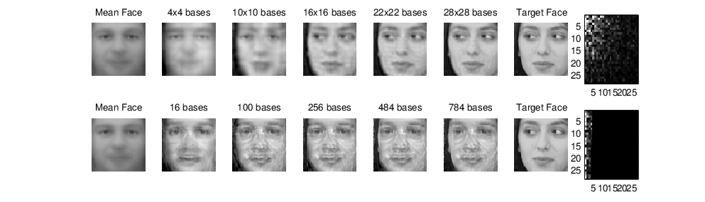
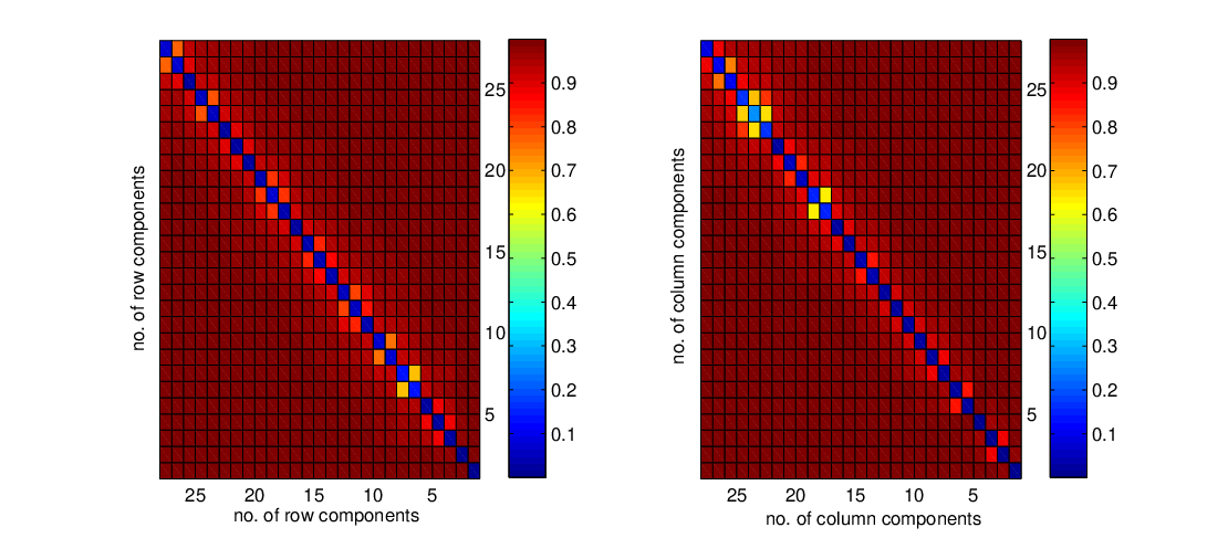
In Figures 1-3, 40 test images are randomly chosen from the test set to show the visual performance of image reconstructions by these two PCA schemes. In MPCA, 28 row eigenvectors and 28 column eigenvectors, both with size 64, are used to generate 784 basis images, of which the 100 leading ones are shown in Figure 4. We remind the reader that the selection $({\tilde{p}},{\tilde{q}})=(28,28)$ produces an $\hat{\rho}({\tilde{p}},{\tilde{q}})$ value $0.968$ . Based on Theorem 3.5, a one-sided $95\%$ confidence interval for $\hat{\rho}(28,28)$ is given by $[0.967,1]$ . We also show the variability pattern plots (Tu and Huang, 2011) in Figure 7. These plots present the average variations (absolute values) of the eigenvectors for the bootstrap re-sampled data, from those eigenvectors for the original data. The horizontal and vertical indices refer to the eigenvector indices for re-sampled and original data. The indices of eigenvectors are sorted by eigenvalues. The variations are presented by colors from dark blue for perfect matched, to dark red for extremely deviated. Usually, eigenvectors with distinct eigenvalues show deep blue on the diagonal and deep red on the off-diagonal. Eigenvectors with the same multiple root eigenvalue tend to be visualized by a cubic pattern on their correspondence indices. It can be seen that our choice of $({\tilde{p}},{\tilde{q}})=(28,28)$ does not produce multiple roots, since the bootstrapped variability of the solutions at this selection is quite small.

In conventional PCA, $784~(=28\times 28)$ eigenvectors (basis images) with size 4096 are used, of which the 100 leading ones are shown in Figure 5. Because of using 100 training images with average subtraction, there are at most 99 meaningful eigenvectors in the conventional PCA. The rest are randomly orthogonal eigenvectors with zero eigenvalue from the remaining subspace. In Figure 5, from top to bottom, we can see the images with clear facial shape to vague ones and a random image on the $100^{\rm th}$ one. On the other hand, MPCA tends to distribute the image characteristics to more basis elements which may allow for more local modification on the images.

In Figure 6, one particular image among the 40 test images is chosen to demonstrate the performance of these two methods. The top row shows the image reconstruction process for MPCA when more basis elements are added in, and the bottom shows for conventional PCA. The mean face is put in the first column and the target image in the $7^{\rm th}$ column as references. The right-most column shows the absolute values of projection scores on the leading 784 basis elements. It is clear that the conventional PCA concentrates on no more than 99 basis elements while the MPCA spreads out to much more basis elements. For MPCA, the image turns its view when $10$ basis elements are used; the pupil turns to left when $16\times 16$ basis elements are used; the double eyelid and nostrils show up when $22\times 22$ basis elements are used; the facial curves become clear when $28\times 28$ basis elements are used. While we can observe the reconstruction progress by adding more basis elements for MPCA, we do not see much difference after 100 basis elements for conventional PCA. It is clear that MPCA performs better than conventional PCA in reconstructing the test images from Table 2 and these figures.

5 Concluding discussions

PCA is a popular tool to reduce the dimensions for high dimensional data analysis; MPCA could be likely to serve the similar function for higher order tensor data sets. From this work, the statistical properties of MPCA become clear through the theoretical framework and the performance of MPCA is predictable through the asymptotic results. Most importantly, based on these asymptotic results, various hypothesis tests become feasible for subsequent analysis, including pattern recognition or classification. Our work, though technically theoretical, may construct a platform to expand the application potentials of MPCA.

The advantages of MPCA over conventional PCA on tensor structure data are evident in the Olivetti Faces data example. Therein, conventional PCA suffers seriously from the large $m$ and small $n$ problem such that there can be at most $n-1$ meaningful eigenvectors. This makes it unavoidable that all the data noises are still carried by the chosen principal components. Furthermore, too concentrated information in one component, which may not be good for pattern recognition or classification prediction. On the other hand, MPCA distributes the information to more components which may allow local modification in the process of image reconstruction, with even fewer free parameters. The key point for the good performance of MPCA is the data tensor structure. For practical purposes, the robustness of MPCA over model variety should be further investigated.

References

: Anderson, T. W. (1963). Asymptotic theory for principal component analysis. Annals of Mathematical Statistics, 34, 122-148.
: De Lathauwer, L., De Moor, B. and Vandewalle, J. (2000a). A multilinear singular value decomposition. SIAM J. Matrix Anal. Appl., 21, 1253-1278.
: De Lathauwer, L., De Moor, B. and Vandewalle, J. (2000b). On the best rank-1 and rank- $(R_{1},R_{2},\dots,R_{N})$ approximation of higher-order tensors. SIAM J. Matrix Anal. Appl., 21, 1324-1342.
: Fine, J. (1987). On the validity of the perturbation method in asymptotic theory. Statistics, 18, 401-414.
: Henderson, H. V. and Searle, S. R. (1979). Vec and vech operators for matrices, with some uses in Jacobians and multivariate statistics. Canadian J. Statistics, 7, 65-81.
: Jolliffe, I.T. (2002). Principal Component Analysis. Springer, New York.
: Kolda, T.G. and Bader, B.W. (2009). Tensor decompositions and applications. SIAM Review, 51(3), 455-500.
: Li, B., Kim, M.K. and Altman, N. (2010). On dimension folding of matrix- or array-valued statistical objects. Annals of Statistics, 38, 1094-1121.
: Lu, H., Plataniotis, K. N. and Venetsanopoulos, A. N. (2008). MPCA: Multilinear principal component analysis of tensor objects. IEEE Transactions on Neural Networks, 19, 18-39.
: Magnus, J. R. and Neudecker, H. (1979). The commutation matrix: some properties and applications. Annals of Statistics, 7, 381-394.
: Sibson, R. (1979). Studies in the robustness of multidimensional scaling: perturbational analysis of classical scaling. J. Roy. Statist. Soc., 41, 217-229.
: Tu, I. P. and Huang, H. C. (2011). An estimation on a covariance matrix when multiple roots exist. manuscript.
: Tyler, D. E. (1981). Asymptotic inference for eigenvectors. Annals of Statistics, 9, 725-736.
: Yang, J., Zhang, D., Frangi, A.F. and Yang, J.Y. (2004). Two-dimensional PCA: a new approach to appearance-based face representation and recognition. IEEE Transactions on Pattern Analysis and Machine Intelligence, 26, 131-137.
: Ye, J. (2005). Generalized low rank approximations of matrices. Machine Learning, 61, 167-191.
: Zhang, D. and Zhou, Z. H. (2005). ${\rm(2D)}^{2}$ PCA: Two-directional two-dimensional PCA for efficient face representation and recognition. Neurocomputing, 69, 224-231.

Appendix

Proof of Proposition 2.2.

In the maximization problem (5), the objective function is continuous and the feasible region ${\cal O}_{q,{\tilde{q}}}\otimes{\cal O}_{p,{\tilde{p}}}$ is compact. (Both continuity and compactness are with respect to the topology induced by Frobenius norm.) Thus, solution(s) exists. ∎

Proof of Proposition 2.5.

(a) Let $[B,\,B_{\perp}]$ be a $q\times q$ orthonormal matrix. Since $B_{0}\in{\rm span}([B,\,B_{\perp}])$ , there exists $\eta_{1}\in\Re^{{\tilde{q}}\times q_{0}}$ and $\eta_{2}\in\Re^{(q-{\tilde{q}})\times q_{0}}$ such that $B_{0}=B\eta_{1}+B_{\perp}\eta_{2}$ . As $B_{0}^{T}B_{0}=I_{q_{0}}$ , we have $\eta_{1}^{T}\eta_{1}+\eta_{2}^{T}\eta_{2}=I_{q_{0}}$ . Observe that

	$\displaystyle E\\|A^{T}(X-\mu)B\\|_{F}^{2}$	(A.1)
$\displaystyle=$	$\displaystyle E\left\{{{\rm trace}}(A^{T}(A_{0}UB_{0}^{T})BB^{T}(B_{0}U^{T}A_{0}^{T})A)\right\}+E\left\{{\rm trace}(A^{T}\varepsilon BB^{T}\varepsilon^{T}A)\right\}$
$\displaystyle=$	$\displaystyle E\left\{{\rm trace}(A^{T}A_{0}U\eta_{1}^{T}\eta_{1}U^{T}A_{0}^{T}A)\right\}+{\tilde{p}}{\tilde{q}}\sigma^{2}$
$\displaystyle=$	$\displaystyle E\left\{{\rm trace}(A^{T}A_{0}UU^{T}A_{0}^{T}A)\right\}-E\left\{{\rm trace}(A^{T}A_{0}U\eta_{2}^{T}\eta_{2}U^{T}A_{0}^{T}A)\right\}+{\tilde{p}}{\tilde{q}}\sigma^{2}$
$\displaystyle\leq$	$\displaystyle E\left\{{\rm trace}(A^{T}A_{0}UU^{T}A_{0}^{T}A)\right\}+{\tilde{p}}{\tilde{q}}\sigma^{2},$

where the equality in (A.1) holds if and only if $\eta_{2}=0$ , if and only if $\eta_{1}^{T}\eta_{1}=I_{q_{0}}$ . Thus, if ${\tilde{q}}\geq q_{0}$ , such an $\eta_{1}$ (with rank $q_{0}$ ) exists to ensure the equality in (A.1). This implies $B_{0}=B\eta_{1}$ and, hence, $B_{0}\in{\rm span}(B)$ . Similarly, $A_{0}\in{\rm span}(A)$ which establishes (a).

To show (b), when ${\tilde{q}}\geq q_{0}$ , from (a) we have $B_{0}\in{\rm span}(B)$ and

\displaystyle\max_{A\in{\cal O}_{p,{\tilde{p}}},B\in{\cal O}_{q,{\tilde{q}}}}E\|A^{T}(X-\mu)B\|_{F}^{2}

\displaystyle=

\displaystyle\max_{A\in{\cal O}_{p,{\tilde{p}}}}{\rm trace}(A^{T}E[A_{0}UU^{T}A_{0}^{T}]A)+{\tilde{p}}{\tilde{q}}\sigma^{2},

(A.2)

which is an eigenvalue-problem for the matrix $E[A_{0}UU^{T}A_{0}^{T}]$ . By diagonalizing $E[UU^{T}]=\Gamma_{U}\Lambda_{U}\Gamma_{U}^{T}$ , then, $E[A_{0}UU^{T}A_{0}^{T}]$ has $p_{0}$ non-zero eigenvalues $\Lambda_{U}$ with the corresponding eigenvectors $A_{0}\Gamma_{U}$ . When ${\tilde{p}}<p_{0}$ , the maximizer $A$ consists of the first ${\tilde{p}}$ columns of $A_{0}\Gamma_{U}$ and, hence, ${\rm span}(A)\subsetneq{\rm span}(A_{0})$ .

To show (d), observe that

E\|A^{T}(X-\mu)B\|_{F}^{2}=E\left\{{\rm trace}(A^{T}A_{0}UB_{0}^{T}BB^{T}B_{0}U^{T}A_{0}^{T}A)\right\}+{\tilde{p}}{\tilde{q}}\sigma^{2}.

(A.3)

To maximize (A.3) over $A\in{\cal O}_{p,{\tilde{p}}},B\in{\cal O}_{q,{\tilde{q}}}$ with ${\tilde{p}}<p_{0}$ and ${\tilde{q}}<q_{0}$ , the rank of $A^{T}A_{0}$ and $B^{T}B_{0}$ must be ${\tilde{p}}$ and ${\tilde{q}}$ , respectively, in order to attain the maximal value. This can happen only if ${\rm span}(A)\subsetneq{\rm span}(A_{0})$ and ${\rm span}(B)\subsetneq{\rm span}(B_{0})$ . ∎

Proof of Proposition 2.6.

We will only provide a proof for (a), and (b) can be obtained in a similar way. If ${\tilde{q}}\geq q_{0}$ , from Proposition 2.5 (a) we have ${\rm span}(B_{0})\subseteq{\rm span}(B)$ , which further implies that

	$\displaystyle E[(X-\mu)P_{B}(X-\mu)^{T}]$	$\displaystyle=$	$\displaystyle E[A_{0}UU^{T}A_{0}^{T}]+E[\varepsilon P_{B}\varepsilon^{T}],$		(A.4)
	$\displaystyle E[(X-\mu)(X-\mu)^{T}]$	$\displaystyle=$	$\displaystyle E[A_{0}UU^{T}A_{0}^{T}]+E[\varepsilon\varepsilon^{T}].$		(A.5)

Note that $E[\varepsilon P_{B}\varepsilon^{T}]={\tilde{q}}\sigma^{2}I_{p}$ and $E[\varepsilon\varepsilon^{T}]=q\sigma^{2}I_{p}$ . Hence, $E[(X-\mu)(X-\mu)^{T}]$ and $E[(X-\mu)P_{B}(X-\mu)^{T}]$ have the same leading $p_{0}\wedge{\tilde{p}}$ eigenvectors as $E[A_{0}UU^{T}A_{0}^{T}]$ has. Moreover, we have $\lambda_{i}=d_{i}+{\tilde{q}}\sigma^{2}$ and $\lambda_{i}^{*}=d_{i}+q\sigma^{2}$ , where $d_{i}$ is the $i^{\rm th}$ eigenvalue of $E[A_{0}UU^{T}A_{0}^{T}]$ . Hence, $\lambda_{i}^{*}-\lambda_{i}=(q-{\tilde{q}})\sigma^{2}$ for $i=1,\dots,{\tilde{p}}$ , which completes the proof. ∎

Proof of Theorem 3.1.

Let ${H_{{\tilde{p}},{\tilde{q}}}}(S_{n})=({\sf vec}(\widehat{A})^{T},{\sf vec}(\widehat{B})^{T})^{T}$ be the function maps $S_{n}$ to its tensor principal components under $({\tilde{p}},{\tilde{q}})$ , which gives ${H_{{\tilde{p}},{\tilde{q}}}}(\Sigma)=({\sf vec}(A)^{T},{\sf vec}(B)^{T})^{T}$ and $D_{H_{{\tilde{p}},{\tilde{q}}}}=\frac{\partial{H_{{\tilde{p}},{\tilde{q}}}}(\Sigma)}{\partial{\sf vec}(\Sigma)}$ . Note that $\widehat{\Phi}(p,q)={\sf vec}(I_{m})^{T}{\sf vec}(S_{n})$ and $\Phi(p,q)={\sf vec}(I_{m})^{T}{\sf vec}(\Sigma)$ . From the weak convergence $\sqrt{n}(S_{n}-\Sigma)\stackrel{{\scriptstyle d}}{{\rightarrow}}N$ and an application of the delta method, we have, for $({\tilde{p}},{\tilde{q}})\leq(p_{0},q_{0})$ ,

$\displaystyle\sqrt{n}\left(\widehat{\Phi}(p,q)-\Phi(p,q)\right)$	$\displaystyle\stackrel{{\scriptstyle d}}{{\to}}$	$\displaystyle{\sf vec}(I_{m})^{T}{\sf vec}(N),$
$\displaystyle\sqrt{n}\left(\widehat{\Phi}({\tilde{p}},{\tilde{q}})-\Phi({\tilde{p}},{\tilde{q}})\right)$	$\displaystyle\stackrel{{\scriptstyle d}}{{\to}}$	$\displaystyle D_{\Phi({\tilde{p}},{\tilde{q}})}{\sf vec}(N),$
$\displaystyle\sqrt{n}\left({H_{{\tilde{p}},{\tilde{q}}}}(S_{n})-{H_{{\tilde{p}},{\tilde{q}}}}(\Sigma)\right)$	$\displaystyle\stackrel{{\scriptstyle d}}{{\to}}$	$\displaystyle D_{H_{{\tilde{p}},{\tilde{q}}}}{\sf vec}(N).$

The explicit forms of $D_{\Phi({\tilde{p}},{\tilde{q}})}$ and elements in $D_{H_{p_{0},q_{0}}}$ are provided in Lemma 3.2. ∎

Proof of Lemma 3.2.

For a given pair $({\tilde{p}},{\tilde{q}})$ with $1\leq{\tilde{p}}\leq p$ and $1\leq{\tilde{q}}\leq q$ , we have, from (6) and (7), that $A$ and $B$ satisfy the following system of stationary equations

	$\displaystyle\left(\sum_{j=1}^{{\tilde{q}}}(b_{j}\otimes I_{p})^{T}\Sigma(b_{j}\otimes I_{p})\right)a_{i}$	$\displaystyle=$	$\displaystyle\lambda_{i}a_{i},~i=1,\cdots,{\tilde{p}},$
	$\displaystyle\left(\sum_{i=1}^{{\tilde{p}}}(I_{q}\otimes a_{i})^{T}\Sigma(I_{q}\otimes a_{i})\right)b_{j}$	$\displaystyle=$	$\displaystyle\xi_{j}b_{j},~j=1,\cdots,{\tilde{q}},$

where $a_{i},b_{j},\lambda_{i},\xi_{j}$ depend on $(\Sigma,{\tilde{p}},{\tilde{q}})$ . The indices $i,j$ in the above system of equations can go beyond ${\tilde{p}}$ and ${\tilde{q}}$ and up to $p$ and $q$ . But those $a_{i}$ and $b_{j}$ with $i>{\tilde{p}}$ and $j>{\tilde{q}}$ will not be included in the solution pair $(A,B)$ . Note that we have the following identity, which is due to the definition of $\Phi$ and the stationary equations:

\Phi({\tilde{p}},{\tilde{q}})=\sum_{i=1}^{\tilde{p}}\lambda_{i}(\Sigma,{\tilde{p}},{\tilde{q}})=\sum_{j=1}^{\tilde{q}}\xi_{j}(\Sigma,{\tilde{p}},{\tilde{q}}).

(A.6)

We will use the perturbation method (Sibson, Lemma 2.1, 1979; Fine, 1987) to derive the derivatives $D_{\Phi({\tilde{p}},{\tilde{q}})}$ , $\frac{\partial a_{i}}{\partial{\sf vec}(\Sigma)}$ and $\frac{\partial b_{j}}{\partial{\sf vec}(\Sigma)}$ . Suppose that $\Sigma$ is perturbed to $\Sigma_{\epsilon}=\Sigma+\epsilon\dot{\Sigma}$ . Denote the corresponding system of stationary equations with $\Sigma_{\epsilon}$ by

	$\displaystyle\left(\sum_{j=1}^{{\tilde{q}}}(b_{j,\epsilon}\otimes I_{p})^{T}\Sigma_{\epsilon}(b_{j,\epsilon}\otimes I_{p})\right)a_{i,\epsilon}$	$\displaystyle=$	$\displaystyle\lambda_{i,\epsilon}~a_{i,\epsilon},~i=1,\cdots,{\tilde{p}},$		(A.7)
	$\displaystyle\left(\sum_{i=1}^{{\tilde{p}}}(I_{q}\otimes a_{i,\epsilon})^{T}\Sigma_{\epsilon}(I_{q}\otimes a_{i,\epsilon})\right)b_{j,\epsilon}$	$\displaystyle=$	$\displaystyle\xi_{j}~b_{j,\epsilon},~j=1,\cdots,{\tilde{q}}.$		(A.8)

Let their first order expansions be denoted by

		$\displaystyle\lambda_{i,\epsilon}=\lambda_{i}+\epsilon\dot{\lambda}_{i}+o(\epsilon),$	$\displaystyle a_{i,\epsilon}=a_{i}+\epsilon\dot{a}_{i}+o(\epsilon),$
		$\displaystyle\xi_{j,\epsilon}=\xi_{j}+\epsilon\dot{\xi}_{j}+o(\epsilon),$	$\displaystyle b_{j,\epsilon}=b_{j}+\epsilon\dot{b}_{j}+o(\epsilon).$

Following the same arguments as in Lemma 2.1 of Sibson (1979) and by equating the terms involving $\epsilon$ in (A.7) we have, for $i=1,\cdots,{\tilde{p}}$ ,

	$\displaystyle\dot{\lambda}_{i}$	$\displaystyle=$	$\displaystyle a_{i}^{T}\dot{\Sigma}_{B}a_{i},$		(A.9)
	$\displaystyle\dot{a}_{i}$	$\displaystyle=$	$\displaystyle\left\{\lambda_{i}I_{p}-\sum_{j=1}^{{\tilde{q}}}(b_{j}\otimes I_{p})^{T}\Sigma(b_{j}\otimes I_{p})\right\}^{+}\dot{\Sigma}_{B}a_{i},$		(A.10)

where

	$\displaystyle\dot{\Sigma}_{B}$	$\displaystyle=$	$\displaystyle\sum_{j=1}^{{\tilde{q}}}\left((\dot{b}_{j}\otimes I_{p})^{T}\Sigma(b_{j}\otimes I_{p})+(b_{j}\otimes I_{p})^{T}\Sigma(\dot{b}_{j}\otimes I_{p})\right)+\sum_{j=1}^{{\tilde{q}}}(b_{j}\otimes I_{p})^{T}\dot{\Sigma}(b_{j}\otimes I_{p})$		(A.11)
		$\displaystyle=$	$\displaystyle E[X(\dot{B}B^{T}+B\dot{B}^{T})X^{T}]+\sum_{j=1}^{{\tilde{q}}}(b_{j}\otimes I_{p})^{T}\dot{\Sigma}(b_{j}\otimes I_{p}).$		(A.11)

Since $B_{\epsilon}^{T}B_{\epsilon}=I_{\tilde{q}}$ , then $\dot{B}=[~\dot{b}_{1},\cdots,\dot{b}_{{\tilde{q}}}~]$ must satisfy $\dot{B}^{T}B+B^{T}\dot{B}=0$ .

(a) For $({\tilde{p}},{\tilde{q}})\leq(p_{0},q_{0})$ , the first term of $\sum_{i=1}^{{\tilde{p}}}a_{i}^{T}\dot{\Sigma}_{B}a_{i}$ can be expressed as

\displaystyle\sum_{i=1}^{{\tilde{p}}}a_{i}^{T}E[X(\dot{B}B^{T}+B\dot{B}^{T})X^{T}]a_{i}

\displaystyle=

\displaystyle\sum_{j=1}^{{\tilde{q}}}\left(\dot{b}_{j}^{T}E[X^{T}P_{A}X]b_{j}+b_{j}^{T}E[X^{T}P_{A}X]\dot{b}_{j}\right)

which vanishes by noting that $b_{j}$ is an eigenvector of $E[XP_{A}X^{T}]$ and $b_{j}^{T}\dot{b}_{j}=\dot{b}_{j}^{T}b_{j}=0$ . This concludes that $\sum_{i=1}^{{\tilde{p}}}\dot{\lambda}_{i}=\sum_{i=1}^{{\tilde{p}}}a_{i}^{T}\left(\sum_{j=1}^{{\tilde{q}}}(b_{j}\otimes I_{p})^{T}\dot{\Sigma}(b_{j}\otimes I_{p})\right)a_{i}$ and, hence,

D_{\Phi({\tilde{p}},{\tilde{q}})}=\sum_{i=1}^{{\tilde{p}}}\sum_{j=1}^{{\tilde{q}}}(b_{j}\otimes a_{i}\otimes b_{j}\otimes a_{i})^{T}={\sf vec}(P_{B\otimes A})^{T}.

(A.12)

(b) Assume now $({\tilde{p}},{\tilde{q}})=(p_{0},q_{0})$ . To derive the form of $\frac{\partial a_{i}}{\partial{\sf vec}(\Sigma)}$ , we are going to show that the first term of $\dot{\Sigma}_{B}$ is zero and conclude $\dot{\Sigma}_{B}=\sum_{j=1}^{q_{0}}(b_{j}\otimes I_{p})^{T}\dot{\Sigma}(b_{j}\otimes I_{p})$ . This together with (A.10) gives

	$\displaystyle\frac{\partial a_{i}}{\partial{\sf vec}(\Sigma)}$	$\displaystyle=$	$\displaystyle\sum_{j=1}^{q_{0}}\left(b_{j}\otimes a_{i}\otimes b_{j}\otimes\{\lambda_{i}I_{p}-E[XP_{B}X^{T}]\}^{+}\right)^{T}$		(A.13)
		$\displaystyle=$	$\displaystyle\left\{a_{i}\otimes{\sf vec}(P_{B_{0}})\otimes(\lambda_{i}I_{p}-E[XP_{B_{0}}X^{T}])^{+}\right\}^{T}(K_{p,q}\otimes I_{pq}).$		(A.13)

as desired, where the second equality follows from Proposition 2.5 that ${\rm span}(B)={\rm span}(B_{0})$ when ${\tilde{q}}=q_{0}$ . To complete the proof, first note that Proposition 2.5 ensures the existence of a nonsingular matrix $\eta$ such that $B_{0}=B\eta$ . From $X=A_{0}UB_{0}^{T}+\varepsilon$ (remember $\mu=0$ ) and the independent structure of $U$ and $\varepsilon$ , we can represent the first term of $\dot{\Sigma}_{B}$ as

	$\displaystyle E[X(\dot{B}B^{T}+B\dot{B}^{T})X^{T}]$	$\displaystyle=$	$\displaystyle E[A_{0}UB_{0}^{T}(\dot{B}B^{T}+B\dot{B}^{T})B_{0}U^{T}A_{0}^{T}]+\sigma^{2}{\rm trace}(B^{T}\dot{B}+\dot{B}^{T}B)I_{p}$
		$\displaystyle=$	$\displaystyle E[A_{0}U\eta^{T}(B^{T}\dot{B}+\dot{B}^{T}B)\eta U^{T}A_{0}^{T}]+\sigma^{2}{\rm trace}(B^{T}\dot{B}+\dot{B}^{T}B)I_{p}.$

The proof is completed by noting that $B^{T}\dot{B}+\dot{B}^{T}B=0$ . The case of $\frac{\partial b_{j}}{\partial{\sf vec}(\Sigma)}$ can be established in a similar way. ∎

Proof of Corollary 3.3.

Consider the function $F(A,B)=P_{B\otimes A}$ with the corresponding differential $D_{F(A,B)}$ . From Theorem 3.1 (b) and delta method, we have

$\displaystyle\sqrt{n}~{\sf vec}(P_{\widehat{B}\otimes\widehat{A}}-P_{B\otimes A})$	$\displaystyle=$	$\displaystyle\sqrt{n}~{\sf vec}(F(\widehat{A},\widehat{B})-F(A,B))$
	$\displaystyle=$	$\displaystyle D_{F(A,B)}\sqrt{n}\left(\left[\begin{array}[]{c}{\sf vec}(\widehat{A})\\ {\sf vec}(\widehat{B})\end{array}\right]-\left[\begin{array}[]{c}{\sf vec}(A)\\ {\sf vec}(B)\end{array}\right]\right)+o(\frac{1}{\sqrt{n}})$
	$\displaystyle\stackrel{{\scriptstyle d}}{{\rightarrow}}$	$\displaystyle D_{P_{B\otimes A}}{\sf vec}(N),$

where $D_{P_{B\otimes A}}=D_{F(A,B)}D_{H_{{\tilde{p}},{\tilde{q}}}}$ . When $({\tilde{p}},{\tilde{q}})=(p_{0},q_{0})$ , the expression of $D_{P_{B\otimes A}}$ is obtained by a direct calculation together with Lemma 3.2 (b) and Theorem 2.5 (a). ∎

Proof of Corollary 3.4.

Consider the function $F(x,y)=x/y$ with the corresponding differential $D_{F(x,y)}=(y^{-1},-xy^{-2})^{T}$ . From Theorem 3.1 (a) and delta method, we have

$\displaystyle\sqrt{n}(\hat{\rho}({\tilde{p}},{\tilde{q}})-\rho({\tilde{p}},{\tilde{q}}))$	$\displaystyle=$	$\displaystyle\sqrt{n}(F(\widehat{\Phi}({\tilde{p}},{\tilde{q}}),\widehat{\Phi}(p,q))-F(\Phi({\tilde{p}},{\tilde{q}}),\Phi(p,q)))$
	$\displaystyle=$	$\displaystyle D_{F(\Phi({\tilde{p}},{\tilde{q}}),\Phi(p,q))}\sqrt{n}\left(\left[\begin{array}[]{c}\widehat{\Phi}({\tilde{p}},{\tilde{q}})\\ \widehat{\Phi}(p,q)\end{array}\right]-\left[\begin{array}[]{c}\Phi({\tilde{p}},{\tilde{q}})\\ \Phi(p,q)\end{array}\right]\right)+o(\frac{1}{\sqrt{n}})$
	$\displaystyle\stackrel{{\scriptstyle d}}{{\rightarrow}}$	$\displaystyle D_{F(\Phi({\tilde{p}},{\tilde{q}}),\Phi(p,q))}\left[\begin{array}[]{c}D_{\Phi({\tilde{p}},{\tilde{q}})}\\ {\sf vec}(I_{m})^{T}\end{array}\right]{\sf vec}(N).$

A direct calculation gives the expression of the asymptotic variance $\sigma^{2}_{\rho({\tilde{p}},{\tilde{q}})}$ . ∎

Proof of Theorem 3.5.

Under $H_{0}$ , we have from Corollary 3.4 that, for $n$ large enough,

\displaystyle P\left(\frac{\sqrt{n}(\hat{\rho}({\tilde{p}},{\tilde{q}})-\rho_{0})}{\sigma_{\rho({\tilde{p}},{\tilde{q}})}}>z_{\alpha}\right)\leq\alpha.

The consistency of $\hat{\sigma}_{\rho({\tilde{p}},{\tilde{q}})}^{2}$ and Slutsky’s theorem complete the proof. ∎

Proof of Theorem 3.6.

Since $({\tilde{p}},{\tilde{q}})=(p_{0},q_{0})$ , we have $A=A^{*}$ and $B=B^{*}$ from Theorem 2.6, and ${\rm span}(A)={\rm span}(A_{0})$ and ${\rm span}(B)={\rm span}(B_{0})$ from Theorem 2.5 (a). Let $\{a_{i}:i>p_{0}\}$ and $\{b_{j}:j>q_{0}\}$ be orthogonal bases of ${\rm span}(Q_{A_{0}})$ and ${\rm span}(Q_{B_{0}})$ , $W_{B,q^{\prime}}=\sum_{j=1}^{q^{\prime}}(b_{j}\otimes I_{p}\otimes b_{j}\otimes I_{p})^{T}$ , $q^{\prime}=1,\cdots,q$ and $W_{A,p^{\prime}}=\sum_{i=1}^{p^{\prime}}(I_{q}\otimes a_{i}\otimes I_{q}\otimes a_{i})^{T}$ , $p^{\prime}=1,\cdots,p$ . Also define $M_{A}=[(a_{1}\otimes M_{A1}),\cdots,(a_{p_{0}}\otimes M_{Ap_{0}})]^{T}$ and $M_{B}=[(b_{1}\otimes M_{B1}),\cdots,(b_{q_{0}}\otimes M_{Bq_{0}})]^{T}$ , where $M_{Ai}=\{\lambda_{i}I_{p}-E[XP_{B_{0}}X^{T}]\}^{+}$ and $M_{Bj}=\{\xi_{j}I_{q}-E[X^{T}P_{A_{0}}X]\}^{+}$ . By using these notations and from Theorem 3.1 (b), we have the limiting distribution of MPCA

\displaystyle\sqrt{n}({\sf vec}(\widehat{A},\widehat{B})-{\sf vec}(A,B))\stackrel{{\scriptstyle d}}{{\rightarrow}}M_{0}W_{0}{\sf vec}(N),

(A.17)

where $M_{0}=\left[\begin{array}[]{cc}M_{A}&0\\ 0&M_{B}\end{array}\right]$ , $W_{0}=\left[\begin{array}[]{c}W_{B,q_{0}}\\ W_{A,p_{0}}\end{array}\right]$ . By Lemma A.1 below, the limiting distribution of $({\rm 2D})^{2}$ PCA is derived to be

\displaystyle\sqrt{n}({\sf vec}(\widehat{A}^{*},\widehat{B}^{*})-{\sf vec}(A^{*},B^{*}))\stackrel{{\scriptstyle d}}{{\rightarrow}}M_{0}(W_{0}+W_{0+}){\sf vec}(N),

(A.18)

where $W_{0+}=\left[\begin{array}[]{c}W_{B,q_{0}+}\\ W_{A,p_{0}+}\end{array}\right]$ , $W_{A,p_{0}+}=W_{A,p}-W_{A,p_{0}}$ , and $W_{B,q_{0}+}=W_{B,q}-W_{B,q_{0}}$ .

Note that $A=A^{*}$ and $B=B^{*}$ . To complete the proof, by an application of delta method, it thus suffices to show

\displaystyle{\rm aCov}({\sf vec}(\widehat{A}^{*},\widehat{B}^{*}))-{\rm aCov}({\sf vec}(\widehat{A},\widehat{B}))\geq 0.

(A.19)

From (A.17)-(A.18) we are left to show

\displaystyle M_{0}(W_{0}\Sigma_{N}W_{0+}^{T}+W_{0+}\Sigma_{N}W_{0}^{T}+W_{0+}\Sigma_{N}W_{0+}^{T})M_{0}^{T}\geq 0,

(A.20)

where $\Sigma_{N}={\rm Cov}({\sf vec}(N))=(I_{m^{2}}+K_{m,m})(\Sigma\otimes\Sigma)$ under normality of ${\sf vec}(X)$ . We are going to show $M_{0}W_{0}\Sigma_{N}W_{0+}^{T}M_{0}^{T}=0$ . This together with the fact $M_{0}W_{0+}\Sigma_{N}W_{0+}^{T}M_{0}^{T}\geq 0$ then establishes the desired result. Observe that

			$\displaystyle M_{0}W_{0}\Sigma_{N}W_{0+}^{T}M_{0}^{T}$
		$\displaystyle=$	$\displaystyle\left[\begin{array}[]{cc}M_{A}W_{B,q_{0}}\Sigma_{N}W_{B,q_{0}+}^{T}M_{A}^{T}&H_{A}W_{B,q_{0}}\Sigma_{N}W_{A,p_{0}+}^{T}M_{B}^{T}\\ H_{B}W_{A,p_{0}}\Sigma_{N}W_{B,q_{0}+}^{T}M_{A}^{T}&H_{B}W_{A,p_{0}}\Sigma_{N}W_{A,p_{0}+}^{T}M_{B}^{T}\end{array}\right].$

From model (1), $\Sigma=(B_{0}\otimes A_{0})(T+\sigma^{2}I_{m_{0}})(B_{0}\otimes A_{0})^{T}+\sigma^{2}Q_{B_{0}\otimes A_{0}}$ , where $Q_{B_{0}\otimes A_{0}}=Q_{B_{0}}\otimes P_{A_{0}}+P_{B_{0}}\otimes Q_{A_{0}}+Q_{B_{0}}\otimes Q_{A_{0}}$ . This implies $W_{B,q_{0}}\Sigma_{N}W_{B,q_{0}+}^{T}=0$ and $W_{A,p_{0}}\Sigma_{N}W_{A,p_{0}+}^{T}=0$ and, hence, the diagonal elements of the above matrix vanish. For the off-diagonal elements, the same reasoning can be used to deduce that $(M_{A}W_{B,q_{0}})\Sigma_{N}W_{A,p_{0}+}^{T}=0$ and $(M_{B}W_{A,p_{0}})\Sigma_{N}W_{B,q_{0}+}^{T}=0$ , which establishes (A.19). A direct calculation further gives

M_{0}W_{0+}\Sigma_{N}W_{0+}^{T}M_{0}^{T}=\sigma^{4}\left[\begin{array}[]{cc}(q-q_{0})M_{A}(I_{p^{2}}+K_{p,p})M_{A}^{T}&0\\ 0&(p-p_{0})M_{B}(I_{q^{2}}+K_{q,q})M_{B}^{T}\end{array}\right],

which equals a zero matrix if and only if $(p_{0},q_{0})=(p,q)$ . ∎

Lemma A.1. Assume model (1) and assume that the leading eigenvalues $\{\lambda_{i}^{*}:i=1,\cdots,p_{0}\}$ and $\{\xi_{j}^{*}:j=1,\cdots,q_{0}\}$ of (2D)²PCA are simple roots. Then, the differentials of (2D)²PCA components with respect to $\Sigma$ under $({\tilde{p}},{\tilde{q}})=(p_{0},q_{0})$ are given by

\displaystyle\frac{\partial{\sf vec}(A^{*})}{\partial{\sf vec}(\Sigma)}=M_{A}W_{B,q}~~~\text{and}~~~\frac{\partial{\sf vec}(B^{*})}{\partial{\sf vec}(\Sigma)}=M_{B}W_{A,p}.

(A.24)

Proof.

We only derive the differential of $A^{*}$ , where the case of $B^{*}$ is similarly obtained. Remember that (2D)²PCA components $A^{*}$ are leading eigenvectors of $K_{A^{*}}=E[XX^{T}]$ with eigenvalues $\lambda_{i}^{*}$ . A standard argument (Sibson, 1979) then gives

	$\displaystyle\frac{\partial{\sf vec}(a_{i}^{})}{\partial{\sf vec}(K_{A^{}})}$	$\displaystyle=$	$\displaystyle a_{i}^{T}\otimes\{\lambda_{i}^{}I_{p}-K_{A^{*}}\}^{+}$		(A.25)
		$\displaystyle=$	$\displaystyle a_{i}^{T}\otimes M_{Ai},$		(A.25)

where the second equality follows from Theorem 2.6 with $M_{Ai}$ being defined in Theorem 3.6. Turning to the differential of $K_{A^{*}}$ with respect to $\Sigma$ . It is always true that

\displaystyle K_{A^{*}}=\sum_{j=1}^{q}(b_{j}\otimes I_{p})^{T}\Sigma(b_{j}\otimes I_{p}),

where $\{b_{j}:j>q_{0}\}$ are defined in the beginning of Theorem 3.6. Thus, we have

\displaystyle\frac{\partial{\sf vec}(K_{A^{*}})}{\partial{\sf vec}(\Sigma)}

\displaystyle=

\displaystyle W_{B,q}.

(A.26)

From (A.25)-(A.26) and the chain rule, the proof is completed. ∎

Refer to caption — Figure 1: 40 test faces randomly drawn from the test set.