跳到论文正文
W Papers独立论文阅读器 arXiv:1104.5268 论文正文 计算阅读时间 · 0%
引用这篇论文根据当前论文元数据生成,正式投稿前建议核对。


License: arXiv.org perpetual non-exclusive license
arXiv:1104.5268v2 [math.PR] 02 Oct 2011

Information Dissemination via Random Walks in dd-Dimensional Space

Henry Lam ††thanks: Department of Mathematics and Statistics, Boston University. Email: khlam@math.bu.edu.    Zhenming Liu ††thanks: Harvard School of Engineering and Applied Sciences. Supported by NSF grant CCF-0915922. Email: zliu@eecs.harvard.edu.    Michael Mitzenmacher ††thanks: Harvard School of Engineering and Applied Sciences. Supported in part by NSF grants CCF-0915922 and IIS-0964473. Email: michaelm@eecs.harvard.edu.    Xiaorui Sun ††thanks: Columbia University. Email: xiaoruisun@cs.columbia.edu.    Yajun Wang ††thanks: Microsoft Research Asia. Email: yajunw@microsoft.com.
Abstract

We study a natural information dissemination problem for multiple mobile agents in a bounded Euclidean space. Agents are placed uniformly at random in the dd-dimensional space {−n,…,n}d\{-n,...,n\}^{d} at time zero, and one of the agents holds a piece of information to be disseminated. All the agents then perform independent random walks over the space, and the information is transmitted from one agent to another if the two agents are sufficiently close. We wish to bound the total time before all agents receive the information (with high probability). Our work extends Pettarin et al’s work [13], which solved the problem for d≤2d\leq 2. We present tight bounds up to polylogarithmic factors for the case d=3d=3. (While our results extend to higher dimensions, for space and readability considerations we provide only the case d=3d=3 here.) Our results show the behavior when d≥3d\geq 3 is qualitatively different from the case d≤2d\leq 2. In particular, as the ratio between the volume of the space and the number of agents varies, we show an interesting phase transition for three dimensions that does not occur in one or two dimensions.

1 Introduction

We study the following information diffusion problem: let a1,a2,…,am\mathrm{a}_{1},\mathrm{a}_{2},...,\mathrm{a}_{m} be mm agents initially starting at locations chosen uniformly at random in 𝒱d={−n,,−(n−1),…,n}d\mathcal{V}^{d}=\{-n,,-(n-1),\ldots,n\}^{d} and performing independent random walks over this space. One of the agents initially has a message, and the message is transmitted from one agent to another when they are sufficiently close. We are interested in the time needed to flood the message, that is, the time when all agents obtain the message. In other settings, this problem has been described as a virus diffusion problem, where the message is replaced by a virus that spreads according to proximity. We use information diffusion and virus spreading interchangeably, depending on which is more useful in context. This is a natural model that has been extensively studied. For example, Alves et al. and Kesten et al. coined the name “frog model” for this problem in the virus setting, and studied the shape formed by the infected contour in the limiting case [1, 2, 10]. In the flooding time setting, early works used a heuristic approximation based on simplifying assumptions to characterize the dynamics of the spread of the message [3, 11, 18]. More recent works provide fully rigorous treatments under this or similar random walk models [5, 6, 13, 16, 12].

The most relevant recent works are those of Pettarin et al. [13] and Peres et al. [12, 16]. The work of Pettarin et al. examines the same model as ours, but their analysis is only for one- and two-dimensional grids. The work of Sinclair and Stauffer [16] considers a similar model they call mobile geometric graphs, and their work extends to higher dimensions. However, their focus and model both have strong differences from ours. For example, they assume a Poisson point process of constant intensity, leading to a number of agents linear in the size of the space. In contrast, our results allow a sublinear number of agents, a scenario not directly relevant to their model. Also, they focus on structural aspects on the mobile graphs, such as percolation, while we are primarily interested in the diffusion time. There are additional smaller differences, but the main point is that for our problem we require and introduce new techniques and analysis.

Our paper presents matching lower bounds and upper bounds (up to polylogarithmic factors) for the flooding problems in dd-dimensional space for an arbitrary constant dd. For ease of exposition, in this paper we focus on the specific case where d=3d=3, which provides the main ideas. Two- and three- dimensional random walks have quite different behaviors – specifically, two-dimensional random walks are recurrent while three-dimensional random walks are transient – so it is not surprising that previous results for two dimensions fail to generalize immediately to three-dimensional space. Our technical contributions include new techniques and tools for tackling the flooding problem by building sharper approximations on the effect of agent interactions. The techniques developed in this paper are also robust enough that our results can be extended to variations of the model, such as allowing probabilistic infection rules, replacing discrete time random walks by continuous time Brownian motions, or allowing the agents to make jumps [6]. These extensions will be reported in future work.

Although the information diffusion problem in three or more dimensions appears less practically relevant than the two-dimensional case, we expect the model will still prove valuable. For instance, particles in a high dimensional space may provide a latent-space representation of the agents in a dynamic social network [8, 14], so understanding information diffusion process may be helpful for designing appropriate latent space models in the future. Also, the problem is mathematically interesting in its own right.

1.1 Our models and results

We follow the model developed in [13]. Let 𝒱d={−n,−(n−1),…,0,…,(n−1),n}d\mathcal{V}^{d}=\{-n,-(n-1),...,0,...,(n-1),n\}^{d} be a dd-dimensional grid. Let A={a1,a2,…,am}A=\{\mathrm{a}_{1},\mathrm{a}_{2},...,\mathrm{a}_{m}\} be a set of moving agents on 𝒱d\mathcal{V}^{d}. At t=0t=0, the agents spread over the space according to some distribution 𝒟\mathcal{D}. Throughout this paper, we focus on the case where 𝒟\mathcal{D} is uniform. Agents move in discrete time steps. Every agent performs a symmetric random walk defined in the natural way. Specifically, at each time step an agent not at a boundary moves to one of its 2​d2d neighbors, each with probability 1/(2​d)1/(2d). If an agent is at a boundary, so there is no edge in one or more directions, we treat each missing edge as a self-loop. Let Ξ1​(t),…,Ξm​(t)∈{0,1}\Xi_{1}(t),...,\Xi_{m}(t)\in\{0,1\} each be a random variable, where Ξi​(t)\Xi_{i}(t) represents whether the agent ai\mathrm{a}_{i} is infected at time step tt. We assume Ξ1​(0)=1\Xi_{1}(0)=1 and Ξi​(0)=0\Xi_{i}(0)=0 for all i≠1i\neq 1. The value Ξi​(t)\Xi_{i}(t) will change from 00 to 11 if at time tt it is within distance 1 to another infected agent aj\mathrm{a}_{j}. (We use distance 1 instead of distance 0 to avoid parity issues.) Once a value Ξj​(t)\Xi_{j}(t) becomes 1, it stays 1.

Definition 1.1.

(Information diffusion problem). Let A1,A2,…,Am∈𝒱dA_{1},A_{2},\ldots,A_{m}\in\mathcal{V}^{d} be the initial positions of the agents a1,…,am\mathrm{a}_{1},\ldots,\mathrm{a}_{m} and let St1​(A1),St2​(A2),…,Stm​(Am)S^{1}_{t}(A_{1}),S^{2}_{t}(A_{2}),\ldots,S^{m}_{t}(A_{m}) be mm independent random walks starting at A1,…,AmA_{1},\ldots,A_{m} respectively, so that Sti​(P)S^{i}_{t}(P) is the position of agent ai\mathrm{a}_{i} at time tt given that at t=0t=0 its position was P∈𝒱dP\in\mathcal{V}^{d}. The infectious state of each agent at time step tt is a binary random variable Ξi​(t)\Xi_{i}(t) such that

  • •

    Ξ1​(0)=1\Xi_{1}(0)=1, Ξi​(0)=0\Xi_{i}(0)=0 for all other ii, and

  • •

    for all t>0t>0, Ξi​(t)=1\Xi_{i}(t)=1 if and only if

    (Ξi(t−1)=1) or (∃j:Ξj(t−1)=1∧‖Sti(Ai)−Stj(Aj)‖1≤1).\left(\Xi_{i}(t-1)=1\right)\quad\mbox{ or }\quad\left(\exists j:\Xi_{j}(t-1)=1\wedge\left\|S^{i}_{t}(A_{i})-S^{j}_{t}(A_{j})\right\|_{1}\leq 1\right).

We define the finishing time of the diffusion process, or the diffusion time, as T=inf{t≥0:|{Ξi(t)=1}|=m}T=\inf\{t\geq 0:|\{\Xi_{i}(t)=1\}|={{m}}\}.

The following results for the diffusion time for 11 and 22 dimensional spaces are proved in [13].

Theorem 1.2.

Consider the information diffusion problem for d=1,2d=1,2 dimensions, and assume the agents are initially uniformly distributed over 𝒱d\mathcal{V}^{d}. Then, with high probability,

T=Θ~(n2⋅m−1/d).T=\tilde{\Theta}(n^{2}\cdot m^{-1/d}). (1)

It is natural to ask whether Equation 1 also holds for d≥3d\geq 3. Our results show this is not the case.

Theorem 1.3.

(Diffusion time for d≥3d\geq 3) Consider the information diffusion problem for d≥3d\geq 3 with initially uniformly distributed agents over 𝒱d\mathcal{V}^{d}. Then there exists a constant cc such that

if c​nd−2​log2​n<m<nd:T=Θ~(nd/2+1⋅m−1/2) with high probability;if m<c​nd−2​log−2​n:T≤Θ~(nd/m) with high prob. and T≥Θ~(nd/m) almost surely.\begin{array}[]{lll}\mbox{if }&cn^{d-2}\log^{2}n<m<n^{d}:&T=\tilde{\Theta}(n^{d/2+1}\cdot m^{-1/2})\mbox{ with high probability;}\\ \mbox{if }&m<cn^{d-2}\log^{-2}n:&T\leq\tilde{\Theta}(n^{d}/m)\mbox{ with high prob. and }T\geq\tilde{\Theta}(n^{d}/m)\mbox{ almost surely.}\end{array} (2)

Notice that Theorems 1.3 and 1.2 yield the same result for d=2d=2, as well as when d=1d=1 and m=Θ⁡(n)m=\Theta(n). Here when we say with high probability, we mean the statement holds with probability 1−n−γ1-n^{-\gamma} for any constant γ\gamma and suitably large nn. When we say almost surely, we mean with probability 1−o⁡(1)1-o(1). When m≥ndm\geq n^{d}, the result is implicit in [10] and the diffusion time in this case is Θ~​(n)\tilde{\Theta}(n). Finally, there are some technical challenges regarding the case c​nd−2​log−2​n≤m≤c​nd−2​log2​ncn^{d-2}\log^{-2}n\leq m\leq cn^{d-2}\log^{2}n that we expect to address in a later version of this work.

An interesting point of our result is that when the number of agents mm is greater than nd−2n^{d-2}, the finishing time is less than the mixing time of each individual random walk, and therefore the analysis requires techniques that do not directly utilize the mixing time. The rest of this paper focuses on deriving both the lower and upper bounds for this interesting case; the case where m<c​nd−2​log−2​nm<cn^{d-2}\log^{-2}n, which harnesses similar ideas and a mixing time argument, is only briefly described at the end. Finally, as previously mentioned, for space reasons we provide only the analysis for the three dimensional case, and note that the results can be generalized to higher dimensions.

Theorem 1.3 can also be expressed in the terms of the density of agents. Let λ=m/nd\lambda=m/n^{d} be the density. We can express the diffusion time as T=Θ~​(n/λ)T=\tilde{\Theta}(n/\sqrt{\lambda}) w.h.p. for c​n−2​log2​n<λ<1cn^{-2}\log^{2}n<\lambda<1, whereas for λ<c​n−2​log−2​n\lambda<cn^{-2}\log^{-2}n we have T≤Θ~​(1/λ)T\leq\tilde{\Theta}(1/\lambda) w.h.p. and T≥Θ~​(1/λ)T\geq\tilde{\Theta}(1/\lambda) almost surely.

We remark that all theorems/propositions/lemmas in this paper are assumed to hold for sufficiently large nn, but for conciseness we may not restate this condition in every instance.

2 Preliminary results for random walks

In this section we lay out some preliminary results on random walks that will be useful in the subsequent sections. These results focus on probabilistic estimates for the meeting time/position of multiple random walks. Along the way, we will also illustrate the limitations of some of these estimates, hence leading to the need of more sophisticated techniques in our subsequent analysis. For conciseness, all proofs in this section are left to Appendix B.

Let 𝐙\mathbf{Z} be the set of integers, and 𝐙3\mathbf{Z}^{3} be the set of integral lattice points in 𝐑3\mathbf{R}^{3}. For two points A,B∈𝐙3A,B\in\mathbf{Z}^{3}, we write A−BA-B as the 33-dimensional vector pointing from BB to AA. For a vector x→∈𝐑3\vec{x}\in\mathbf{R}^{3}, denote the iith coordinate of x→\vec{x} as xix_{i}. Define the LpL_{p} norm of a vector as ‖x→‖p=(∑i≤3|xi|p)1/p\|\vec{x}\|_{p}=\left(\sum_{i\leq 3}|x_{i}|^{p}\right)^{1/p}, and also the infinite-norm in the standard manner ‖x→‖∞=maxi≤3⁡|xi|\|\vec{x}\|_{\infty}=\max_{i\leq 3}|x_{i}|. We moderately overload xx in this paper, i.e. xx is a scalar and x→\vec{x} is a vector.

Let S1S^{1} and S2S^{2} be two random walks in either 𝒱3\mathcal{V}{{{}^{3}}} (bounded walks) or 𝐙3\mathbf{Z}^{3} (unbounded walks). We say two walks S1S^{1} and S2S^{2} meet at time tt if their L1L_{1}-distance is within 11 at that time and two walks S1S^{1} and S2S^{2} collide at tt if they are exactly at the same position at time tt.

Definition 2.1 (Passage probability).

Let SS be a random walk in 𝐙3\mathbf{Z}^{3} starting at the origin OO. Let BB be a point with B−O=x→B-O=\vec{x} (which is a three dimensional vector). Define the probability that SS is at BB at time tt as p⁡(t,x→)p(t,\vec{x}). Define the probability that SS visits BB within time tt as q⁡(t,x→)q(t,\vec{x}).

We want to characterize the chance that two or more random walks in either 𝒱3\mathcal{V}{{{}^{3}}} or 𝐙3\mathbf{Z}^{3} meet. More specifically, consider the following question. Let A1A_{1}, …, AjA_{j}, and BB be j+1j+1 points over the 3-dimensional space 𝐙3\mathbf{Z}^{3} such that for all i∈[j]i\in[j], the L1L_{1} distance between AiA_{i} and BB is ‖Ai−B‖1≥x\|A_{i}-B\|_{1}\geq x. Let S1​(A1),…,Sj​(Aj)S^{1}(A_{1}),...,S^{j}(A_{j}), Sj+1​(B)S^{j+1}(B) be independent random walks that start with these points respectively. Our goal is to understand the probability that all the walks S1S^{1}, …, SjS^{j} will meet or collide with the random walk Sj+1S^{j+1} within x2x^{2} time steps. We note that if the agents starting at BB was stationary instead of following its own random walk then the analysis of the situation would be straightforward. In particular, the probability that all the walks would intersect BB is Θ~​(1/xk)\tilde{\Theta}(1/x^{k}). This follows from standard results, including Theorem A.10 and Lemma A.11 provided in the appendices. We need to consider a more challenging situation when the agent starting at BB is also moving.

To begin, we shall consider the case where j=1{{j}}=1, so that we have just two moving agents.

Definition 2.2.

Let AA and BB be two points over 𝐙3\mathbf{Z}^{3} such that A−B=x→A-B=\vec{x}. where ‖x→‖1\|\vec{x}\|_{1} is an even number. Let S1S^{1} and S2S^{2} be two independent unbounded random walks that start at AA and BB respectively. Define Q⁡(t,x→)Q(t,\vec{x}) as the probability that S1S^{1} and S2S^{2} collide before time tt.

We can use a simple coupling argument to relate Q⁡(t,x→)Q(t,\vec{x}) with q⁡(t,x→)q(t,\vec{x}). The result is described as follows.

Lemma 2.3.

Let AA and BB be two points over 𝐙3\mathbf{Z}^{3} such that A−B=x→A-B=\vec{x}, where ‖x→‖1\|\vec{x}\|_{1} is an even number. Consider Q⁡(t,x→)Q(t,\vec{x}) and q⁡(t,x→)q(t,\vec{x}) defined above. We have Q⁡(t,x→)=q⁡(2​t,x→)Q(t,\vec{x})=q(2t,\vec{x}). Furthermore, for t≥‖x→‖22t\geq\|\vec{x}\|^{2}_{2}, Q⁡(t,x→)=Θ⁡(1/‖x→‖2)Q(t,\vec{x})=\Theta(1/\|\vec{x}\|_{2}).

Next, let us move to the case of jj random walks in 𝐙3\mathbf{Z}^{3}, in which j>1j>1.

Lemma 2.4.

Let A1A_{1}, A2A_{2}, …, AjA_{j}, and BB be points in 𝐙3\mathbf{Z}^{3} such that ‖Ai−B‖1\|A_{i}-B\|_{1} are even and ‖Ai−B‖1≥x\|A_{i}-B\|_{1}\geq x for all i≤ji\leq j. Let S1​(A1),…,Sj​(Aj)S^{1}(A_{1}),\ldots,S^{j}(A_{j}), Sj+1​(B)S^{j+1}(B) be j+1j+1 independent random walks that start at A1,…,Aj,BA_{1},\ldots,A_{j},B respectively. Let t=x2t=x^{2}. Then the probability that all the walks S1,…,SjS^{1},\ldots,S^{j} collide with St+1S^{t+1} within time tt is at most (ζ​jx)j\left(\frac{\zeta j}{x}\right)^{j}, where ζ\zeta is a sufficiently large constant.

Lemma 2.4 also helps us to analyze the scenario in which agents need to meet rather than to collide. This is summarized by the following corollary:

Corollary 2.5.

Let A1A_{1}, A2A_{2}, …, AjA_{j}, and BB be points in 𝐙3\mathbf{Z}^{3} such that ‖Ai−B‖1≥x\|A_{i}-B\|_{1}\geq x for all i≤ji\leq j. Let S1​(A1),…,Sj​(Aj)S^{1}(A_{1}),...,S^{j}(A_{j}), Sj+1​(B)S^{j+1}(B) be j+1j+1 independent random walks that start at A1,…,Aj,BA_{1},...,A_{j},B respectively. Let t=x2t=x^{2}. Then the probability that all the walks S1,…,SjS^{1},...,S^{j} meet with Sj+1S^{j+1} within time tt is at most (ζ′​jx)j\left(\frac{\zeta^{\prime}j}{x}\right)^{j}, where ζ′\zeta^{\prime} is a sufficiently large constant.

We note that both Lemma 2.4 and Corollary 2.5 are useful only when xx is large enough. This forms a barrier for analysis of close agents in our model. But as we will see, we can get around this issue by looking at a coupled diffusion process that possesses a different diffusion rule specifically designed for handling close agents.

Another important issue is the analysis on walks that are close to the boundary. For this, we show that the random walks will not behave significantly different (in terms of the desired bounds) when boundaries are added. We notice that similar results are presented in [13], but their results do not immediately translate to the building blocks we need here. The following is the major building block we need for our analysis:

Lemma 2.6.

Let AA and BB be two points in 𝒱3\mathcal{V}^{3} such that A−B=x→A-B=\vec{x} and the distance between AA and any boundary is at least 40​‖x→‖140\|{{\vec{x}}}\|_{1}. Consider two random walks S1​(A)S^{1}(A) and S2​(B)S^{2}(B) that start at AA and BB respectively. Let e~t\tilde{e}_{t} be the event that S1​(A)S^{1}(A) and S2​(B)S^{2}(B) will meet before time t=‖x→‖12t{{=\|\vec{x}\|_{1}^{2}}} and before either of them visits a boundary. Then Pr⁡[e~‖x→‖12]=Ω⁡(1/‖x→‖1)\Pr[\tilde{e}_{\|{{\vec{x}}}\|_{1}^{2}}]=\Omega(1/\|{{\vec{x}}}\|_{1}).

3 Lower bound

Let us first state our lower bound result more precisely as follows.

Theorem 3.1.

Let a1,…,am\mathrm{a}_{1},...,\mathrm{a}_{m} be placed uniformly at random on 𝒱3\mathcal{V}^{3} such that 1600​n​log2⁡n≤m≤n31600n\log^{2}n\leq m\leq n^{3}. Let ℓ2=n3/m\ell_{2}=\sqrt{n^{3}/m}. For sufficiently large nn, the diffusion time TT satisfies the following inequality

Pr[T≤181ℓ2nlog−29n]≤exp(−lognloglogn).\Pr[T\leq\frac{1}{81}\ell_{2}n\log^{-29}n]\leq\exp\left(-\log n\log\log n\right).

We use a local analysis to prove our lower bound. The key idea is that under uniform distribution of agents, the extent any particular infected agent can spread the virus within a small time increment is confined to a small neighborhood with high probability. By gluing together these local estimates, we can approximate the total diffusion time.

To explain our local analysis, assume we start with an arbitrary infected agent, say a1\mathrm{a}_{1}. Let us also assume, for simplicity, that all the other uniformly distributed agents are uninfected. Consider the scenario within a small time increment, say Δ​t\Delta t. During this time increment the agent a1\mathrm{a}_{1} infects whoever it meets in the small neighborhood that contains its extent of movement. The newly infected agents then continue to move and infect others. The size of the final region that contains all the infected agents at Δ​t\Delta t then depends on the rate of transmission and the extent of movement of all of the infected agents. In particular, if Δ​t\Delta t is small enough, the expected number of transmissions performed by a1\mathrm{a}_{1} is less than one; even if it infects another agent, the number of infections it causes within the same Δ​t\Delta t is also less than one, and so on. The net effect is an eventual dying-out of this “branching process” (which we later model by what we call a diffusion tree), which localizes the positions of all infected agents at time Δ​t\Delta t to a small neighborhood around the initial position of a1\mathrm{a}_{1}.

As it may not be clear as we go through our proofs, we briefly review the main methodologies in obtaining lower bound results in related work, and point out their relation to our analysis and difficulties in directly applying them to higher dimensions. (Some readers may wish to skip these next paragraphs all together; for others, who would like a more thorough discussion that unavoidably requires more technical details, we devote Appendix E to more details.) Two potential existing methods arise in [2, 10] and [13]. The former analyzes the growth rate of the size of the total infected region; an upper bound on this growth rate translates to a lower bound for the diffusion time. The latter work, focusing on d=1,2d=1,2, uses an “island diffusion rule”, which essentially speeds up infection by allowing infections to occur immediately on connected components in an underlying graph where edges are based on the distance between agents. This approach avoids handling the issue of the meeting time of random walks when they are very close, a regime where asymptotic results such as Lemma 2.3 and 2.4 may not apply, while still providing a way to bound the diffusion time by arguing about the low probability of interaction among different “islands”.

The results in [2, 10] are not directly applicable in our setting because the growth rate they obtain is linear in time, as a result of their assumption of constant agent density in an infinite space, in contrast to our use of a size parameter nn that scales with the agent density. It is fairly simple to see that blindly applying a linear growth rate to our setting of o⁡(1)o(1) density is too crude. On the other hand, analyzing how agent density affects the growth rate is a potentially feasible approach but certainly not straightforward.

Our approach more closely follows [13]. The main limitation of [13], when applied to higher dimension, is how to control the interaction among islands. If islands interact too often, because they are too close together, the argument, which is based on a low probability of interaction, breaks down. However, if one parametrizes islands to prevent such interaction, then the bound that can be obtained are too weak. In Appendix E.1 we provide further details arguing that for d>2d>2 this constraint ultimately limits the analysis for the case of o⁡(1)o(1) density. We attempt to remedy the problem by using islands as an intermediate step to obtain local estimates of the influence of each initially infected agent over small periods of time. This analysis involves looking at a branching process representing the spread of the infection, significantly extending the approach of [13].

3.1 Local diffusion problem

This subsection focuses on the local analysis as discussed above. In Section 3.2, we will proceed to discuss how to utilize this analysis to get the lower bound in Theorem 3.1. As discussed in the last section, the two main difficulties in our analysis are: 1) our probabilistic estimates for the meeting time/position of multiple random walks are only useful asymptotically; 2) walks near the boundary introduce further analytical complication. To begin with, the following definition serves to handle the second issue:

Definition 3.2 (Interior region).

The interior region 𝔙⁡(r)\mathfrak{V}(r) parameterized by rr is the set of lattice points in 𝒱3\mathcal{V}^{3} that have at least L∞L_{\infty}-distance rr to the boundary.

For any point P∈𝒱3P\in{\mathcal{V}}^{3}, define 𝔹⁡(P,x)={Q∈𝒱3:‖Q−P‖∞≤x}\mathbb{B}(P,x)=\{Q\in\mathcal{V}^{3}:\|Q-P\|_{\infty}\leq x\} as the xx-ball of neighborhood of PP under L∞L_{\infty}-norm. The following proposition is our major result in this subsection.

Proposition 3.3.

Consider a diffusion following Definition 1.1. Let S0S_{0} be the initial position of the only infected agent a1\mathrm{a}_{1} at time 0, and 𝒲\mathcal{W} be an arbitrary subset of lattice points in 𝔙⁡(20​ℓ2​log⁡n)\mathfrak{V}(20\ell_{2}\log n), where ℓ2=n3/m\ell_{2}=\sqrt{n^{3}/m}. Denote Δ​t=ℓ22​log−28​n\Delta t=\ell^{2}_{2}\log^{-28}n. Define the binary random variable b⁡(𝒲)b(\mathcal{W}) as follows:

  • •

    If S0∈𝒲S_{0}\in\mathcal{W}: b⁡(𝒲)b(\mathcal{W}) is set as 1 if and only if all the infected agents at time Δ​t\Delta t can be covered by the ball 𝔹⁡(S0,9​ℓ2​log⁡n)\mathbb{B}(S_{0},9\ell_{2}\log n).

  • •

    If S0∉𝒲S_{0}\notin\mathcal{W}: b⁡(𝒲)=1b(\mathcal{W})=1.

We have

Pr[b(𝒲)=1]≥1−exp(−5lognloglogn)\Pr[b(\mathcal{W})=1]\geq 1-\exp(-5\log n\log\log n) (3)

The proposition yields that with high probability, all the infected agents lie within a neighborhood of distance O~​(ℓ2)\tilde{O}(\ell_{2}) at time O~​(ℓ22)\tilde{O}(\ell_{2}^{2}). The variable ℓ2\ell_{2} is chosen such that the expected number of infections spanned by an initially infected agent a1\mathrm{a}_{1} within O~​(ℓ22)\tilde{O}(\ell_{2}^{2}) units of time and a neighborhood of O~​(ℓ2)\tilde{O}(\ell_{2}) distance is O⁡(1)O(1). This can be seen by solving m​(ℓ2/n)3×(1/ℓ2)=O~​(1)m(\ell_{2}/n)^{3}\times(1/\ell_{2})=\tilde{O}(1), where m​(ℓ2/n)3m(\ell_{2}/n)^{3} is the expected number of agents in a cube of size ℓ2×ℓ2×ℓ2\ell_{2}\times\ell_{2}\times\ell_{2}, and O~​(1/ℓ2)\tilde{O}(1/\ell_{2}) is the meeting probability within time O~​(ℓ22)\tilde{O}(\ell_{2}^{2}) between any pair of random walks with initial distance ℓ2\ell_{2} (see Lemma 2.3). This choice of ℓ2\ell_{2} appears to be the right threshold for our analysis. Indeed, a larger scale than ℓ2\ell_{2} would induce a large number of infections made by a1\mathrm{a}_{1}, and also subsequent infections made by newly infected agents, with an exploding affected region as an end result. On the other hand, a smaller scale than ℓ2\ell_{2} would degrade our lower bound. This is because the diffusion time is approximately of order n/ℓ2n/\ell_{2}, the number of spatial steps to cover 𝒱3\mathcal{V}^{3}, times ℓ22\ell_{2}^{2}, the time taken for each step, equaling n​ℓ2n\ell_{2}. Hence a decrease in ℓ2\ell_{2} weakens the bound11 1 In the case of general dd-dimensional space, ℓ2\ell_{2} is chosen such that m​(ℓ2/n)d×(1/ℓ2d−2)=O~​(1)m(\ell_{2}/n)^{d}\times(1/\ell_{2}^{d-2})=\tilde{O}(1), giving ℓ2=nd/m\ell_{2}=\sqrt{n^{d}/m}. Throughout the paper such dd-dimensional analog can be carried out in similar fashion, but for ease of exposition we shall not bring up these generalizations and will focus on the 3-dimensional case..

Secondly, we introduce 𝒲\mathcal{W} in Proposition 3.3 to avoid the case when S0S_{0} is close to the boundary. As we have mentioned, such boundary conditions often complicate random walk analysis. Although the impact of the boundary’s presence has been addressed (e.g., [6, 13]), existing results are not fully satisfactory. For example, when two simple random walks S1S^{1} and S2S^{2} start near the boundary, only a lower bound for the probability that two walks meet within a specific number of time steps is available ([13]); we do not know of an upper bound counterpart. We arrange our proof so that it is sufficient to analyze the diffusion pattern of a virus when it starts far from the boundary. Finally, we note that no effort has been made to optimize the exponent 28 in Δ​t\Delta t’s definition.

We briefly explain how our global lower bound can be readily obtained from Proposition 3.3, which is a strong characterization of the local growth rate of infection region size. Imagine the following evolution. Starting with a single infected agent, with high probability the infection spreads to a ball of radius at most 9​ℓ2​log⁡n9\ell_{2}\log n in Δ​t\Delta t time units. At this time point, the newly infected agents inside the ball continue to spread the virus to neighborhoods of size at most 9​ℓ2​log⁡n9\ell_{2}\log n, again with high probability. This gives an enlarged area of infection with radius at most 18​ℓ2​log⁡n18\ell_{2}\log n. Continuing in this way, the lower bound in Theorem 1.3 is then the time for the infection to spread over 𝒱3\mathcal{V}^{3}. This observation will be made rigorous in the next subsection.

The rest of this subsection is devoted to the proof of Proposition 3.3. It consists of two main steps. First, we need to estimate the expected number of infections done by a single initially infected agent within distance 9​ℓ2​log⁡n9\ell_{2}\log n and time increment Δ​t\Delta t. Second, we iterate to consider each newly infected agent. The analysis requires the condition that the global configuration behaves “normally”, a scenario that occurs with suitably high probability, as we show. We call this condition “good behavior”, which is introduced through the several definitions below:

Definition 3.4.

(Island, [13]) Let A={a1,…,am}A=\{\mathrm{a}_{1},...,\mathrm{a}_{m}\} be the set of agents in 𝒱3\mathcal{V}^{3}. For any positive integer γ>0\gamma>0, let Gt​(γ)G_{t}(\gamma) be the graph with vertex set AA such that there is an edge between two vertices if and only if the corresponding agents are within distance γ\gamma (under L1L_{1}-norm) at time tt. The island with parameter γ\gamma of an agent ai∈A\mathrm{a}_{i}\in A at time step tt, denoted by Isdt​(ai,γ)\mathrm{Isd}_{t}(\mathrm{a}_{i},\gamma) is the connected component of Gt​(γ)G_{t}(\gamma) containing ai\mathrm{a}_{i}.

Definition 3.5 (Good behavior).

Let ℓ1=nm−1/3\ell_{1}=nm^{-1/3}. For 1≤i≤(ℓ2/ℓ1)​log−3​n1\leq i\leq(\ell_{2}/\ell_{1})\log^{-3}n, define ℬi​(P)=𝔹⁡(P,i​ℓ1​log−1​n)\mathcal{B}_{i}(P)=\mathbb{B}\left(P,i\ell_{1}\log^{-1}n\right) and let ∂ℬi​(P)=ℬi​(P)−ℬi−1​(P)\partial\mathcal{B}_{i}(P)=\mathcal{B}_{i}(P)-\mathcal{B}_{i-1}(P). For any P∈𝒱3P\in\mathcal{V}^{3}, define mi​(P)=(log5⁡n)​|∂ℬi​(P)|​m(2​n+1)3m_{i}(P)=\frac{(\log^{5}n)|\partial\mathcal{B}_{i}(P)|m}{(2n+1)^{3}}. Let us define the following binary random variables:

  • •

    Good density. Let {Dt:t≥0}\{D_{t}:t\geq 0\} be a sequence of 0,10,1 random variables such that Dt=1D_{t}=1 if and only if for all P∈𝒱3P\in\mathcal{V}^{3} and all i≤(ℓ2/ℓ1)​log−3​ni\leq(\ell_{2}/\ell_{1})\log^{-3}n, the number of agents in ∂ℬi​(P)\partial\mathcal{B}_{i}(P) is at most mi​(P)m_{i}(P), for all time steps up to tt. We say the diffusion process has the good density property at time tt if Dt=1D_{t}=1.

  • •

    Small islands. Let {Et:t≥0}\{E_{t}:t\geq 0\} be a sequence of 0,10,1 random variables such that Et=1E_{t}=1 if and only if |Isds​(aj,ℓ1​log−1​n)|≤3​log⁡n|{\mathrm{Isd}}_{s}(\mathrm{a}_{j},\ell_{1}\log^{-1}n)|\leq 3\log n for all aj∈A\mathrm{a}_{j}\in A and 0≤s≤t0\leq s\leq t. We say that the diffusion process has the small islands property at time tt if Et=1E_{t}=1.

  • •

    Short travel distance. Let {Lt:t≥0}\{L_{t}:t\geq 0\} be a sequence of 00, 11 random variables such that Lt=1L_{t}=1 if and only if for all i∈[m]i\in[m] and all t1<t2≤tt_{1}<t_{2}\leq t with t2−t1≤ℓ22​log−12​nt_{2}-t_{1}\leq\ell^{2}_{2}\log^{-12}n, we have ‖St1i−St2i‖1≤3​ℓ2​log−4​n\|S^{i}_{t_{1}}-S^{i}_{t_{2}}\|_{1}\leq 3\ell_{2}\log^{-4}n. We say the process has the short travel distance property at time tt if Lt=1L_{t}=1.

Finally, let Gt=Dt×Et×LtG_{t}=D_{t}\times E_{t}\times L_{t}, and say the diffusion process behaves well at time tt if Gt=1G_{t}=1. We also focus on t≤n2.5t\leq n^{2.5} and define the random variable G=Gn2.5G=G_{n^{2.5}}.

The value n2.5n^{2.5} in the definition is chosen such that it lies well beyond our lower bound for the case m<n3m<n^{3}, but is small enough for our forthcoming union bound. By using properties of random walks and techniques derived in  [13], we have

Lemma 3.6.

Let A={a1,…,am}A=\{\mathrm{a}_{1},...,\mathrm{a}_{m}\} be agents that are distributed uniformly in 𝒱3\mathcal{V}^{3} at t=0t=0. For sufficiently large nn, we have Pr[G=1]≥1−exp(−6lognloglogn)\Pr[G=1]\geq 1-\exp(-6\log n\log\log n).

The proof of Lemma 3.6 is presented in Appendix C. With this global “good behavior”, we have the following estimate:

Lemma 3.7.

Let A={a1,…,am}A=\{\mathrm{a}_{1},\ldots,\mathrm{a}_{m}\} be agents that are distributed in 𝒱3{\mathcal{V}}^{3} in such a way that D0=1D_{0}=1. Let S1,S2,…,SmS^{1},S^{2},\ldots,S^{m} be their corresponding random walks. Consider an arbitrary agent aj\mathrm{a}_{j} with S0j∈𝔙⁡(2​ℓ2​log−4​n)S^{j}_{0}\in\mathfrak{V}(2\ell_{2}\log^{-4}n). Let {ai1,…,aik}\{\mathrm{a}_{i_{1}},\ldots,\mathrm{a}_{i_{k}}\} be the set of agents outside ℬ1​(S0j)\mathcal{B}_{1}(S^{j}_{0}) at time 00. Define Xj,ℓX_{j,\ell} as the indicator random variable that represents whether the agents aj\mathrm{a}_{j} and aiℓ\mathrm{a}_{i_{\ell}} meet within time [0,Δ​t][0,\Delta t]. We have

E[∑ℓ≤kXj,ℓ|D0=1,S0j∈𝔙(2ℓ2log−4n)]<log−3n.\mathrm{E}\left[\sum_{\ell\leq k}X_{j,\ell}\Bigg|D_{0}=1,S^{j}_{0}\in\mathfrak{V}(2\ell_{2}\log^{-4}n)\right]<\log^{-3}n.
Proof.

First, notice that the number of lattice points in ∂ℬi​(P)\partial\mathcal{B}_{i}(P) satisfies

|∂ℬi|=|ℬi|−|ℬi−1|≤(2​i​ℓ1​log−1​n)3−(2​(i−1)​ℓ1​log−1​n)3≤24​i2​ℓ13​log−3​n.|\partial\mathcal{B}_{i}|=|\mathcal{B}_{i}|-|\mathcal{B}_{i-1}|\leq(2i\ell_{1}\log^{-1}n)^{3}-(2(i-1)\ell_{1}\log^{-1}n)^{3}\leq 24i^{2}\ell^{3}_{1}\log^{-3}n.

We may also similarly show that

|∂ℬi|≥i2​ℓ13​log−3​n.|\partial\mathcal{B}_{i}|\geq i^{2}\ell_{1}^{3}\log^{-3}n.

Let q=(ℓ2/ℓ1)​log−3​nq=(\ell_{2}/\ell_{1})\log^{-3}n. For each i∈[q]i\in[q], write ℬi=ℬ⁡(S0j)\mathcal{B}_{i}=\mathcal{B}(S^{j}_{0}), ∂ℬi=∂ℬi​(S0j)\partial\mathcal{B}_{i}=\partial\mathcal{B}_{i}(S^{j}_{0}), and mi=mi​(S0j)m_{i}=m_{i}(S^{j}_{0}). We want to estimate the meeting probability and hence the expected number of infections for each i∈[q]i\in[q].

First, let us consider the agents outside the ball ℬq\mathcal{B}_{q}. The probability that any specific agent initially outside ℬq\mathcal{B}_{q} ever travels into the ball 𝔹⁡(S0j,ℓ2​log−4​n)\mathbb{B}(S^{j}_{0},\ell_{2}\log^{-4}n) within time ℓ22​log−12​n\ell^{2}_{2}\log^{-12}n is at most exp⁡(−Ω⁡(log3⁡n))\exp(-\Omega(\log^{3}n)) ( by, e.g., Lemma A.6 in the section on probability review). On the other hand, the probability that SjS^{j} ever travels out of 𝔹⁡(S0j,ℓ2​log−4​n)\mathbb{B}(S^{j}_{0},\ell_{2}\log^{-4}n) is also exp⁡(−Ω⁡(log3⁡n))\exp(-\Omega(\log^{3}n)). For these two agents to meet, at least one of these events has to occur. Therefore, with probability exp⁡(−Ω⁡(log3⁡n))\exp(-\Omega(\log^{3}n)) SjS^{j} will meet an agent initially outside ℬq\mathcal{B}_{q}. This leads to

E[∑ik′:S0ik′∉ℬqXj,k′⏟the set of agents initially outside ℬq|D0=1,S0j∈𝔙(2ℓ2log−4n)]≤mexp(−Ω(log3n)).\mathrm{E}\Bigg[\underbrace{\sum_{i_{k^{\prime}}:S^{i_{k^{\prime}}}_{0}\notin\mathcal{B}_{q}}X_{j,k^{\prime}}}_{\begin{subarray}{c}\mbox{the set of agents initially }\\ \mbox{outside $\mathcal{B}_{q}$}\end{subarray}}\Bigg|D_{0}=1,S^{j}_{0}\in\mathfrak{V}(2\ell_{2}\log^{-4}n)\Bigg]\leq m\exp(-\Omega(\log^{3}n)).

Let us next focus on agents inside ℬq\mathcal{B}_{q}. Fix an arbitrary aiℓ∈∂ℬi\mathrm{a}_{i_{\ell}}\in\partial\mathcal{B}_{i}. Let eje^{j} and eℓe^{\ell} represents the events that SjS^{j} and Siℓ{{S^{{i}_{\ell}}}} ever visit a boundary before time ℓ22​log−12​n\ell^{2}_{2}\log^{-12}n respectively. Again by Lemma A.6, Pr[ej∨eℓ|D0=1,S0j∈𝔙(2ℓ2log−4n)]=exp(−Ω(log3n))\Pr[e^{j}\vee e^{\ell}|D_{0}=1,S^{j}_{0}\in\mathfrak{V}(2\ell_{2}\log^{-4}n)]=\exp(-\Omega(\log^{3}n)). We now have

E[Xj,ℓ|D0=1,S0j∈𝔙(2ℓ2log−4n)]\displaystyle\mathrm{E}[X_{j,\ell}|D_{0}=1,S^{j}_{0}\in\mathfrak{V}(2\ell_{2}\log^{-4}n)]
=\displaystyle= Pr[Xj,ℓ=1;¬ej∧¬eℓ|D0=1,S0j∈𝔙(2ℓ2log−4n)]+Pr[Xj,ℓ=1;ej∨eℓ|D0=1,S0j∈𝔙(2ℓ2log−4n)]\displaystyle\Pr[X_{j,\ell}=1;\neg e^{j}\wedge\neg e^{\ell}|D_{0}=1,S^{j}_{0}\in\mathfrak{V}(2\ell_{2}\log^{-4}n)]+\Pr[X_{j,\ell}=1;e^{j}\vee e^{\ell}|D_{0}=1,S^{j}_{0}\in\mathfrak{V}(2\ell_{2}\log^{-4}n)]
≤\displaystyle\leq Pr[Xj,ℓ=1;¬ej∧¬eℓ|D0=1,S0j∈𝔙(2ℓ2log−4n)]+exp(−Ω(log3n)).\displaystyle\Pr[X_{j,\ell}=1;\neg e^{j}\wedge\neg e^{\ell}|D_{0}=1,S^{j}_{0}\in\mathfrak{V}(2\ell_{2}\log^{-4}n)]+\exp(-\Omega(\log^{3}n)).

To compute

Pr[Xj,ℓ;¬ej∧¬eℓ|D0=1,S0j∈𝔙(2ℓ2log−4n)]\displaystyle\Pr[X_{j,\ell};\neg e^{j}\wedge\neg e^{\ell}|D_{0}=1,S^{j}_{0}\in\mathfrak{V}(2\ell_{2}\log^{-4}n)]
=\displaystyle= Pr[{∃t0≤ℓ22log12⁡n:∥St0j−St0iℓ∥1≤1}⋀(¬ej∧¬eℓ)|D0=1,S0j∈𝔙(2ℓ2log−4n)],\displaystyle\Pr\left[\left\{\exists t_{0}\leq\frac{\ell^{2}_{2}}{\log^{12}n}:\|S^{j}_{t_{0}}-S^{i_{\ell}}_{t_{0}}\|_{1}\leq 1\right\}\bigwedge\left(\neg e^{j}\wedge\neg e^{\ell}\right)\Bigg|D_{0}=1,S^{j}_{0}\in\mathfrak{V}(2\ell_{2}\log^{-4}n)\right],

we couple SjS^{j} and Siℓ{{S^{i_{\ell}}}} with unbounded walks 𝐒j\mathbf{S}^{j} and 𝐒iℓ{{\mathbf{S}^{i_{\ell}}}} starting at the same positions at t=0t=0 in the natural way. Before the pair of bounded walks visit the boundary, they coincide with their unbounded counterparts. Therefore, we have

Pr[{∃t0≤ℓ22log12⁡n:∥St0j−St0iℓ∥1≤1}⋀(¬ej∧¬eℓ)|D0=1,S0j∈𝔙(2ℓ2log−4n)]\displaystyle\Pr\left[\left\{\exists t_{0}\leq\frac{\ell^{2}_{2}}{\log^{12}n}:\|S^{j}_{t_{0}}-S^{i_{\ell}}_{t_{0}}\|_{1}\leq 1\right\}\bigwedge\left(\neg e^{j}\wedge\neg e^{\ell}\right)\Bigg|D_{0}=1,S^{j}_{0}\in\mathfrak{V}(2\ell_{2}\log^{-4}n)\right]
≤\displaystyle\leq Pr[∃t0≤ℓ22log12⁡n:∥𝐒t0j−𝐒t0iℓ∥1≤1|D0=1,S0j∈𝔙(2ℓ2log−4n)]=O(1(i−1)​ℓ1)(Corollary 2.5)\displaystyle Pr\left[\exists t_{0}\leq\frac{\ell^{2}_{2}}{\log^{12}n}:\|\mathbf{S}^{j}_{t_{0}}-\mathbf{S}^{i_{\ell}}_{t_{0}}\|_{1}\leq 1\Bigg|D_{0}=1,S^{j}_{0}\in\mathfrak{V}(2\ell_{2}\log^{-4}n)\right]=O(\frac{1}{(i-1)\ell_{1}})\hskip 9.24994pt\mbox{(Corollary~\ref{cor:rwcatchall})}

We thus have E[Xj,ℓ|D0=1,S0j∈𝔙(2ℓ2log−4n)]≤C0(i−i)​ℓ1\mathrm{E}[X_{j,\ell}|D_{0}=1,S^{j}_{0}\in\mathfrak{V}(2\ell_{2}\log^{-4}n)]\leq\frac{C_{0}}{(i-i)\ell_{1}} for some constant C0C_{0}. Next, we estimate Ei≡E[∑ℓ:S0iℓ∈∂ℬiXj,ℓ∣D0=1,S0j∈𝔙(2ℓ2log−4n)]\mathrm{E}_{i}\equiv\mathrm{E}[\sum_{\ell:S^{i_{\ell}}_{0}\in\partial\mathcal{B}_{i}}X_{j,\ell}\mid D_{0}=1,S^{j}_{0}\in\mathfrak{V}(2\ell_{2}\log^{-4}n)] as

Ei≤C0​mi(i−1)​ℓ1=C0(i−1)​ℓ1⋅|∂ℬi|​m​log5​n8​n3=C0​(3​i2​ℓ13​log−3​n)​m​log5​n(i−1)​ℓ1​n3≤6​C0​i​m​ℓ12​log2​nn3.\mathrm{E}_{i}\leq\frac{C_{0}m_{i}}{(i-1)\ell_{1}}=\frac{C_{0}}{(i-1)\ell_{1}}\cdot\frac{|\partial\mathcal{B}_{i}|m\log^{5}n}{8n^{3}}=\frac{C_{0}(3i^{2}\ell^{3}_{1}\log^{-3}n)m\log^{5}n}{(i-1)\ell_{1}n^{3}}\leq\frac{6C_{0}im\ell^{2}_{1}\log^{2}{{n}}}{n^{3}}.

The first inequality holds because D0=1D_{0}=1 and mim_{i} is an upper bound for the number of agents in ∂ℬi\partial\mathcal{B}_{i} (for all ii).

E[∑ℓ≤kXj,ℓ∣D0=1,S0j∈𝔙(2ℓ2log−4n)]\displaystyle\mathrm{E}[\sum_{\ell\leq k}X_{j,\ell}\mid D_{0}=1,S^{j}_{0}\in\mathfrak{V}(2\ell_{2}\log^{-4}n)] ≤\displaystyle\leq ∑i≤qEi+m×exp⁡(−Ω⁡(log3⁡n))⏟upper bound for those outside ​Bq\displaystyle\sum_{i\leq q}\mathrm{E}_{i}+\underbrace{m\times\exp(-\Omega(\log^{3}n))}_{\mbox{upper bound for those outside }\mathbb{\mathcal{}}B_{q}}
≤\displaystyle\leq (∑2≤i≤qi)​6​C0​m​ℓ12​log2​nn3+exp⁡(−Ω⁡(log2⁡n))\displaystyle\left(\sum_{2\leq i\leq q}i\right)\frac{6C_{0}m\ell^{2}_{1}\log^{2}n}{n^{3}}+\exp(-\Omega(\log^{2}n))
<\displaystyle< 6​C0​q2​m​ℓ12​log2​nn3+exp⁡(−Ω⁡(log2⁡n))\displaystyle\frac{6C_{0}q^{2}m\ell^{2}_{1}\log^{2}n}{n^{3}}+\exp(-\Omega(\log^{2}n))
=\displaystyle= 6​C0​log−4​n+exp⁡(−Ω⁡(log2⁡n))\displaystyle 6C_{0}\log^{-4}n+\exp(-\Omega(\log^{2}n))
<\displaystyle< log−3⁡n\displaystyle\log^{-3}n

for sufficiently large nn as m<n3m<n^{3}. ∎

Lemma 3.7 says that if the initial distribution of agents possesses good behavior, then one can ensure that the expected number of direct infections on far-away agents is small. For agents close to the initially infected agents, we instead utilize the concept of islands, which is also deeply related to the subsequent virus spreading behavior. Now we formally introduce a new diffusion process with a modified “island diffusion” rule. It is easy to see that this new diffusion process can be naturally coupled with the original diffusion process (evolving with Definition 1.1) by using the same random walks in the same probability space.

Definition 3.8 (Diffusion process with island diffusion rule).

Consider a diffusion process in which mm agents are performing random walks on 𝒱3\mathcal{V}^{3}. An uninfected agent aj\mathrm{a}_{j} becomes infected at time tt if one of the following conditions holds:

  1. 1.

    it meets a previously infected agent at time tt. For convenience, we say aj\mathrm{a}_{j} is directly infected if it is infected in this way.

  2. 2.

    it is inside Isdt​(ai,ℓ1​log−1​n){\mathrm{Isd}}_{t}(\mathrm{a}_{i},\ell_{1}\log^{-1}n) where ai\mathrm{a}_{i} is directly infected at time tt.

This coupled process is different from the diffusion models introduced in  [13, 16, 12]. In our formulation, an island is infected only if meeting occurs between one uninfected and one previously infected agent. In  [13, 16, 12] (using our notations), an island is infected once it contains a previously infected agent. As a result, infections occur less frequently in our model than the models in  [13, 16, 12]. This difference is the key to getting a tight lower bound for dimensions higher than 2. More precisely, our infection rule allows us to build a terminating branching process, or what we call “diffusion tree” in the following definition, whose generations are defined via the infection paths from the source. The termination of this branching process constrains the region of infection to a small neighborhood around the source with a probability of larger order than obtained in [13]. This in turn leads to a tighter global lower bound.

Definition 3.9 (Diffusion tree).

Let 𝒲⊆𝔙⁡(2​ℓ2​log⁡n)\mathcal{W}\subseteq\mathfrak{V}(2\ell_{2}\log n) be a subset of lattice points. Consider a diffusion, following the island diffusion rule, that starts with an initially infected island Isd0​(a1,ℓ1​log−1​n){\mathrm{Isd}}_{0}(\mathrm{a}_{1},\ell_{1}\log^{-1}n). Recall that S01S^{1}_{0} denotes a1\mathrm{a}_{1}’s position at t=0t=0. The diffusion tree Tr{\mathrm{Tr}} with respect to 𝒲\mathcal{W} has the following components:

  1. 1.

    If S01∉𝒲S^{1}_{0}\notin\mathcal{W}, Tr=∅{\mathrm{Tr}}=\emptyset.

  2. 2.

    If S01∈𝒲S^{1}_{0}\in\mathcal{W},

    • •

      The root of Tr{\mathrm{Tr}} is a dummy node rr.

    • •

      The children of rr are all the agents in Isd0​(a1,ℓ1​log−1​n){\mathrm{Isd}}_{0}(\mathrm{a}_{1},\ell_{1}\log^{-1}n).

    • •

      aℓ′\mathrm{a}_{\ell^{\prime}} is a child of aℓ\mathrm{a}_{\ell} (aℓ′∈child⁡(aℓ)\mathrm{a}_{\ell^{\prime}}\in{\mathrm{child}}(\mathrm{a}_{\ell})) if aℓ′\mathrm{a}_{\ell^{\prime}} is infected by aℓ\mathrm{a}_{\ell} before time Δ​t\Delta t.

    • •

      aℓ′\mathrm{a}_{\ell^{\prime}} is a direct child of aℓa_{\ell} (aℓ′∈dchild⁡(aℓ)\mathrm{a}_{\ell^{\prime}}\in\mathrm{dchild}(\mathrm{a}_{\ell})) if aℓ′∈child⁡(aℓ)\mathrm{a}_{\ell^{\prime}}\in{\mathrm{child}}(\mathrm{a}_{\ell}) and it is directly infected by aℓ\mathrm{a}_{\ell}.

For technical reasons, if aℓ′\mathrm{a}_{\ell^{\prime}} is not in Tr{\mathrm{Tr}}, we let child⁡(aℓ)=∅{\mathrm{child}}(\mathrm{a}_{\ell})=\emptyset and dchild⁡(aℓ)=∅\mathrm{dchild}(\mathrm{a}_{\ell})=\emptyset.

Figure 1 in the Appendix shows an example of the diffusion process and its corresponding diffusion tree at t=0,20,40,60t=0,20,40,60. Notice that the diffusion tree Tr{\mathrm{Tr}} stops growing after Δ​t\Delta t steps.

We refer the root of the tree as the 00th level of the tree and count levels in the standard way. The height of the tree is the number of levels in the tree. Note that diffusion tree defined in this way can readily be interpreted as a branching process (See, e.g., Chapter 0 in [19]), in which the jjth generation of the process corresponds with the jjth level nodes in Tr{\mathrm{Tr}}.

Next we incorporate the good behavior variable GtG_{t} with diffusion tree. The motivation is that, roughly speaking, consistently good behavior guarantees a small number of infections, or creation of children, at each level. This can be seen through Lemma 3.7.

Definition 3.10 (Stopped diffusion tree).

Consider a diffusion process with island diffusion rule, and let T⁡(ℓ)T(\ell) be the time that aℓ\mathrm{a}_{\ell} becomes infected in the process. The stopped diffusion tree Tr′{\mathrm{Tr}}^{\prime} (with respect to ai\mathrm{a}_{i} and 𝒲\mathcal{W}) is a subtree of Tr{\mathrm{Tr}} induced by the set of vertices {aℓ:aℓ∈Tr∧GT⁡(ℓ)=1}\{\mathrm{a}_{\ell}:\mathrm{a}_{\ell}\in{\mathrm{Tr}}\ \wedge\ G_{T(\ell)}=1\}. We write aℓ∈child′​(aℓ′)\mathrm{a}_{\ell}\in{\mathrm{child}}^{\prime}(\mathrm{a}_{\ell^{\prime}}) if aℓ∈child⁡(aℓ′)\mathrm{a}_{\ell}\in{\mathrm{child}}(\mathrm{a}_{\ell^{\prime}}) and aℓ∈Tr′\mathrm{a}_{\ell}\in{\mathrm{Tr}}^{\prime}. Similarly, aℓ∈dchild′​(aℓ′)\mathrm{a}_{\ell}\in\mathrm{dchild}^{\prime}(\mathrm{a}_{\ell^{\prime}}) if aℓ∈dchild⁡(aℓ′)\mathrm{a}_{\ell}\in\mathrm{dchild}(\mathrm{a}_{\ell^{\prime}}) and aℓ∈Tr′\mathrm{a}_{\ell}\in{\mathrm{Tr}}^{\prime}.

Note that the definition of stopped diffusion tree involves global behavior of the whole diffusion process due to the introduction of GtG_{t}. On the other hand, Tr=Tr′{\mathrm{Tr}}={\mathrm{Tr}}^{\prime} with overwhelming probability, so we can translate the properties of Tr′{\mathrm{Tr}}^{\prime} back to Tr{\mathrm{Tr}} easily.

We next show two properties of the (stopped) diffusion trees, one on the physical propagation of children relative to their parents and one on the tree height. These are our main ingredients for proving Proposition 3.3. The properties are in brief:

  1. 1.

    If aℓ\mathrm{a}_{\ell} is a child of aℓ′\mathrm{a}_{\ell^{\prime}} in the stopped diffusion tree Tr′{\mathrm{Tr}}^{\prime}, ‖ST⁡(ℓ)ℓ−ST⁡(ℓ′)ℓ′‖∞\|S^{\ell}_{T(\ell)}-S^{\ell^{\prime}}_{T(\ell^{\prime})}\|_{\infty} is O~​(ℓ2)\tilde{O}(\ell_{2}).

  2. 2.

    The height of the stopped diffusion tree Tr′{\mathrm{Tr}}^{\prime} is O~​(1)\tilde{O}(1) with high probability.

Proving the first item requires the following notion:

Definition 3.11 (Generation distance).

Consider the diffusion tree Tr{\mathrm{Tr}} with respect to 𝒲\mathcal{W}. Let aℓ\mathrm{a}_{\ell} be an arbitrary agent and let aℓ′\mathrm{a}_{\ell^{\prime}} be its parent on Tr{\mathrm{Tr}}. The generation distance of aℓ\mathrm{a}_{\ell} with respect to Tr{\mathrm{Tr}} is

𝔡ℓ={‖ST⁡(ℓ)ℓ−ST⁡(ℓ′)ℓ′‖1 if aℓ is in Tr and is at the 2nd or deeper level0 otherwise.\mathfrak{d}_{\ell}=\left\{\begin{array}[]{ll}\|S^{\ell}_{T(\ell)}-S^{\ell^{\prime}}_{T(\ell^{\prime})}\|_{1}&\mbox{ if $\mathrm{a}_{\ell}$ is in ${\mathrm{Tr}}$ and is at the 2nd or deeper level}\\ 0&\mbox{ otherwise.}\end{array}\right. (4)

In other words, the generation distance between aℓ\mathrm{a}_{\ell} and aℓ′\mathrm{a}_{\ell^{\prime}} is the distance between where aℓ\mathrm{a}_{\ell} and aℓ′\mathrm{a}_{\ell^{\prime}} were infected. The generation distance of aℓ\mathrm{a}_{\ell} with respect to Tr′{\mathrm{Tr}}^{\prime} is 𝔡ℓ′\mathfrak{d}^{\prime}_{\ell}, which is set to be 𝔡ℓ\mathfrak{d}_{\ell} if aℓ\mathrm{a}_{\ell} is in Tr′{\mathrm{Tr}}^{\prime} and 00 otherwise.

With this notion, we can derive the following lemma:

Lemma 3.12.

Consider the stopped diffusion tree with respect to 𝒲\mathcal{W} that starts with an infected island Isd0​(ai,ℓ1​log−1​n){\mathrm{Isd}}_{0}(\mathrm{a}_{i},\ell_{1}\log^{-1}n). For an agent aℓ\mathrm{a}_{\ell} in Tr′{\mathrm{Tr}}^{\prime}, 𝔡ℓ′≤4​ℓ2\mathfrak{d}^{\prime}_{\ell}\leq 4\ell_{2}.

Proof.

We focus on the non-trivial case that S0i∈𝒲S_{0}^{i}\in\mathcal{W} and that aℓ\mathrm{a}_{\ell} is at the 2nd level of Tr′{\mathrm{Tr}}^{\prime} or deeper. Suppose that the diffusion process behaves well up to time T⁡(ℓ)T(\ell) i.e. GT⁡(ℓ)=1G_{T(\ell)}=1. Let aℓ′\mathrm{a}_{\ell^{\prime}} be the parent of aℓ\mathrm{a}_{\ell} on Tr′{\mathrm{Tr}}^{\prime}. By the construction of Tr′{\mathrm{Tr}}^{\prime}, there exists an aℓ′′∈dchild′​(aℓ′)\mathrm{a}_{\ell^{\prime\prime}}\in\mathrm{dchild}^{\prime}(\mathrm{a}_{\ell^{\prime}}) (possibly aℓ\mathrm{a}_{\ell} itself) such that

  • •

    aℓ∈IsdT⁡(ℓ′′)​(aℓ′′,ℓ1​log−1​n)\mathrm{a}_{\ell}\in{\mathrm{Isd}}_{T(\ell^{\prime\prime})}(\mathrm{a}_{\ell^{\prime\prime}},\ell_{1}\log^{-1}n).

  • •

    T⁡(ℓ)=T⁡(ℓ′′)T(\ell)=T(\ell^{\prime\prime}) i.e., aℓ\mathrm{a}_{\ell} and aℓ′′\mathrm{a}_{\ell^{\prime\prime}} get infected at the same time due to the island diffusion rule.

  • •

    ‖ST⁡(ℓ)ℓ′−ST⁡(ℓ)ℓ′′‖1≤1\|S^{\ell^{\prime}}_{T(\ell)}-S^{\ell^{\prime\prime}}_{T(\ell)}\|_{1}\leq 1 i.e., aℓ′′\mathrm{a}_{\ell^{\prime\prime}} gets infected because it meets an infected agent.

By the triangle inequality,

𝔡ℓ′=‖ST⁡(ℓ′)ℓ′−ST⁡(ℓ)ℓ‖1≤‖ST⁡(ℓ′)ℓ′−ST⁡(ℓ′′)ℓ′′‖1+‖ST⁡(ℓ′′)ℓ′′−ST⁡(ℓ)ℓ‖1.\mathfrak{d}_{\ell}^{\prime}=\|S^{\ell^{\prime}}_{T(\ell^{\prime})}-S^{\ell}_{T(\ell)}\|_{1}\leq\|S^{\ell^{\prime}}_{T(\ell^{\prime})}-S^{\ell^{\prime\prime}}_{T(\ell^{\prime\prime})}\|_{1}+\|S^{\ell^{\prime\prime}}_{T(\ell^{\prime\prime})}-S^{\ell}_{T(\ell)}\|_{1}.

Note that ‖ST⁡(ℓ′)ℓ′−ST⁡(ℓ′′)ℓ′′‖1≤3​ℓ2​log−4​n+1≤ℓ2\|S^{\ell^{\prime}}_{T(\ell^{\prime})}-S^{\ell^{\prime\prime}}_{T(\ell^{\prime\prime})}\|_{1}\leq 3\ell_{2}\log^{-4}n+1\leq\ell_{2} (short travel distance property) and ‖ST⁡(ℓ′′)ℓ′′−ST⁡(ℓ)ℓ‖1≤(ℓ1​log−1​n)​(3​log⁡n)=3​ℓ1≤3​ℓ2\|S^{\ell^{\prime\prime}}_{T(\ell^{\prime\prime})}-S^{\ell}_{T(\ell)}\|_{1}\leq(\ell_{1}\log^{-1}n)(3\log n)=3\ell_{1}\leq 3\ell_{2} (small island property) since GT⁡(ℓ)=1G_{T(\ell)}=1. Finally, the case when GT⁡(ℓ)=0G_{T(\ell)}=0 is trivial, and the lemma follows. ∎

Next we show that with high probability the height of the stopped diffusion tree is O~​(1)\tilde{O}(1). Using standard notation, we let {ℱt}t≥0\{\mathcal{F}_{t}\}_{t\geq 0} be the σ\sigma-algebra, or filtration, generated up to time tt, i.e., ℱt\mathcal{F}_{t} encodes all the information regarding the diffusion process up to tt. The special instance ℱ0\mathcal{F}_{0} is used to describe the initial positions of the agents.

The main property of stopped diffusion tree that we need is the following:

Lemma 3.13.

Consider a diffusion process with the island diffusion rule. Let aℓ\mathrm{a}_{\ell} be an arbitrary agent with infection time T⁡(ℓ)T(\ell). We have

E[|dchild′(aℓ)||ℱT⁡(ℓ),ST⁡(ℓ)ℓ∈𝔙(2ℓ2log−4n)]≤log−3n,\mathrm{E}\left[|\mathrm{dchild}^{\prime}(\mathrm{a}_{\ell})|\Big|\mathcal{F}_{T(\ell)},S^{\ell}_{T(\ell)}\in\mathfrak{V}(2\ell_{2}\log^{-4}n)\right]\leq\log^{-3}n, (5)

where dchild′​(⋅)\mathrm{dchild}^{\prime}(\cdot) is defined for a stopped diffusion tree with respect to an arbitrary set 𝒲⊆𝔙⁡(20​ℓ2​log⁡n)\mathcal{W}\subseteq\mathfrak{V}(20\ell_{2}\log n).

We regard the conditional expectation in Equation 5 as a random variable. The interpretation is that the expected number of aℓ\mathrm{a}_{\ell}’s direct children is less than log−3⁡n\log^{-3}n, regardless of the global configuration at the infection time of aℓ\mathrm{a}_{\ell}, as long as it lies in 𝔙⁡(2​ℓ2​log−4​n)\mathfrak{V}(2\ell_{2}\log^{-4}n) at that time.

Proof.

We focus on the case when S01∈𝒲S^{1}_{0}\in\mathcal{W}; otherwise Tr′{\mathrm{Tr}}^{\prime} is empty and the lemma trivially holds. First observe that all aj∈IsdT⁡(ℓ)​(ST⁡(ℓ)ℓ,ℓ1​log−1​n)\mathrm{a}_{j}\in{\mathrm{Isd}}_{T(\ell)}(S^{\ell}_{T(\ell)},\ell_{1}\log^{-1}n) are infected at or before the time aℓ\mathrm{a}_{\ell} is infected. Therefore they cannot be direct children of aℓ\mathrm{a}_{\ell} by Definition 3.9 and 3.10. On the other hand, an agent aj\mathrm{a}_{j} is outside IsdT⁡(ℓ)​(ST⁡(ℓ)ℓ,ℓ1​log−1​n){\mathrm{Isd}}_{T(\ell)}(S^{\ell}_{T(\ell)},\ell_{1}\log^{-1}n) only if it is outside the ball 𝔹⁡(ST⁡(ℓ)ℓ,ℓ1​log−1​n)\mathbb{B}(S^{\ell}_{T(\ell)},\ell_{1}\log^{-1}n). Hence dchild′​(aℓ)\mathrm{dchild}^{\prime}(\mathrm{a}_{\ell}) is bounded by the number of agents initially outside 𝔹⁡(ST⁡(ℓ)ℓ,ℓ1​log−1​n)\mathbb{B}(S^{\ell}_{T(\ell)},\ell_{1}\log^{-1}n) that meet aℓ\mathrm{a}_{\ell} before time Δ​t\Delta t. We consider two cases:

Case 1. DT⁡(ℓ)=1D_{T(\ell)}=1. By Lemma 3.7, we have

E[|dchild′(aℓ)||ℱT⁡(ℓ),DT⁡(ℓ)=1,ST⁡(ℓ)ℓ∈𝔙(2ℓ2log−4n)]≤log−3n.\mathrm{E}\left[|\mathrm{dchild}^{\prime}(\mathrm{a}_{\ell})|\Big|\mathcal{F}_{T(\ell)},D_{T(\ell)}=1,S^{\ell}_{T(\ell)}\in\mathfrak{V}(2\ell_{2}\log^{-4}n)\right]\leq\log^{-3}n.

Case 2. DT⁡(ℓ)=0D_{T(\ell)}=0. By Definition 3.10, we have

E[|dchild′(aℓ)||ℱT⁡(ℓ),DT⁡(ℓ)=0,ST⁡(ℓ)ℓ∈𝔙(2ℓ2log−4n)]=0≤log−3n.\mathrm{E}\left[|\mathrm{dchild}^{\prime}(\mathrm{a}_{\ell})|\Big|\mathcal{F}_{T(\ell)},D_{T(\ell)}=0,S^{\ell}_{T(\ell)}\in\mathfrak{V}(2\ell_{2}\log^{-4}n)\right]=0\leq\log^{-3}n.

Therefore,

E[|dchild′(aℓ)||ℱT⁡(ℓ),ST⁡(ℓ)ℓ∈𝔙(2ℓ2log−4n)]\displaystyle\mathrm{E}\left[|\mathrm{dchild}^{\prime}(\mathrm{a}_{\ell})|\Big|\mathcal{F}_{T(\ell)},S^{\ell}_{T(\ell)}\in\mathfrak{V}(2\ell_{2}\log^{-4}n)\right] =\displaystyle= EℱT⁡(ℓ)[E[|dchild′(aℓ)||ℱT⁡(ℓ),ST⁡(ℓ)ℓ∈𝔙(2ℓ2log−4n),DT⁡(ℓ)]]\displaystyle\mathrm{E}_{\mathcal{F}_{T(\ell)}}\left[\mathrm{E}\left[|\mathrm{dchild}^{\prime}(\mathrm{a}_{\ell})|\Big|\mathcal{F}_{T(\ell)},S^{\ell}_{T(\ell)}\in\mathfrak{V}(2\ell_{2}\log^{-4}n),D_{T(\ell)}\right]\right]
≤\displaystyle\leq log−3⁡n.\displaystyle\log^{-3}n.

∎

Recursive utilization of Lemma 3.13 on successive tree levels leads to the following lemma:

Lemma 3.14.

Consider a diffusion process with the island diffusion rule starting with an infected island Isd(a1,ℓ1log−1n)0{\mathrm{Isd}}{{{}_{0}}}(\mathrm{a}_{1},\ell_{1}\log^{-1}n). For the stopped diffusion tree Tr′{\mathrm{Tr}}^{\prime} with respect to any 𝒲⊆𝔙⁡(20​ℓ2​log⁡n)\mathcal{W}\subseteq\mathfrak{V}(20\ell_{2}\log n), let Height⁡(Tr′)\mathrm{Height}({\mathrm{Tr}}^{\prime}) be its height. Then we have

Pr[Height(Tr′)>2logn]≤exp(−3lognloglogn).\Pr[\mathrm{Height}({\mathrm{Tr}}^{\prime})>2\log n]\leq\exp(-3\log n\log\log n). (6)

Let us denote the set of agents at the kkth level as 𝔽k\mathbb{F}_{k}. It is worth pointing out that, despite a similar analysis to that of standard branching process, there is a technical complication on the conditioning argument since the creation of each child within the same level can be performed at different times in the diffusion process. This implies that there is no single filtration that we can condition on each level to analyze the expected size of the next one. Nevertheless, conditioning can be tailored to each agent at the same level.

Proof.

We focus on the case when Tr′{\mathrm{Tr}}^{\prime} is non-trivial i.e. S01∈𝒲S_{0}^{1}\in\mathcal{W}. Let I⁡(A)=1I(A)=1 if AA occurs and 0 otherwise. We have, for any k<2​log⁡nk<2\log n,

E[|𝔽k+1′||ℱ0,S01∈𝒲]\displaystyle\mathrm{E}[|\mathbb{F}^{\prime}_{k+1}||\mathcal{F}_{0},S_{0}^{1}\in\mathcal{W}]
=\displaystyle= E[∑aℓ∈𝔽k′∑aℓ′∈dchild′​(aℓ)|IsdT⁡(ℓ′)(aℓ′,ℓ1log−1n)|I(GT⁡(ℓ′)=1)|ℱ0,S01∈𝒲]\displaystyle\mathrm{E}\left[\sum_{\mathrm{a}_{\ell}\in\mathbb{F}^{\prime}_{k}}\sum_{\mathrm{a}_{\ell^{\prime}}\in\mathrm{dchild}^{\prime}(\mathrm{a}_{\ell})}|{\mathrm{Isd}}_{T(\ell^{\prime})}(\mathrm{a}_{\ell^{\prime}},\ell_{1}\log^{-1}n)|I(G_{T(\ell^{\prime})}=1)\mathbf{\Bigg|}\mathcal{F}_{0},S^{1}_{0}\in\mathcal{W}\right]
≤\displaystyle\leq (3logn)E[∑aℓ∈𝔽k′|dchild′(aℓ)||ℱ0,S01∈𝒲]\displaystyle(3\log n)\mathrm{E}\left[\sum_{\mathrm{a}_{\ell}\in\mathbb{F}^{\prime}_{k}}|\mathrm{dchild}^{\prime}(\mathrm{a}_{\ell})|\mathbf{\Bigg|}\mathcal{F}_{0},S^{1}_{0}\in\mathcal{W}\right]

The equality holds by the stopping rule and the inequality holds by the small islands property. Next we have

E[∑aℓ∈𝔽k′|dchild′(aℓ)||ℱ0,S01∈𝒲]\displaystyle\mathrm{E}\left[\sum_{\mathrm{a}_{\ell}\in\mathbb{F}^{\prime}_{k}}|\mathrm{dchild}^{\prime}(\mathrm{a}_{\ell})|\mathbf{\Bigg|}\mathcal{F}_{0},S^{1}_{0}\in\mathcal{W}\right]
=\displaystyle= E[∑ℓ∈[m]I(aℓ∈𝔽k′)|dchild′(aℓ)||ℱ0,S01∈𝒲]\displaystyle\mathrm{E}\left[\sum_{\ell\in[m]}I(\mathrm{a}_{\ell}\in\mathbb{F}^{\prime}_{k})|\mathrm{dchild}^{\prime}(\mathrm{a}_{\ell})|\mathbf{\Bigg|}\mathcal{F}_{0},S^{1}_{0}\in\mathcal{W}\right]
=\displaystyle= ∑ℓ∈[m]E[I(aℓ∈𝔽k′)|dchild′(aℓ)||ℱ0,S01∈𝒲]\displaystyle\sum_{\ell\in[m]}\mathrm{E}\left[I(\mathrm{a}_{\ell}\in\mathbb{F}^{\prime}_{k})|\mathrm{dchild}^{\prime}(\mathrm{a}_{\ell})|\mathbf{\Bigg|}\mathcal{F}_{0},S^{1}_{0}\in\mathcal{W}\right]
=\displaystyle= ∑ℓ∈[m]E[E[I(aℓ∈𝔽k′)|dchild′(aℓ)||ℱT⁡(ℓ),S01∈𝒲]|ℱ1,S01∈𝒲]\displaystyle\sum_{\ell\in[m]}\mathrm{E}\left[\mathrm{E}\left[I(\mathrm{a}_{\ell}\in\mathbb{F}^{\prime}_{k})|\mathrm{dchild}^{\prime}(\mathrm{a}_{\ell})|\mathbf{\Bigg|}\mathcal{F}_{T(\ell)},S^{1}_{0}\in\mathcal{W}\right]\Bigg|\mathcal{F}_{1},S^{1}_{0}\in\mathcal{W}\right]
=\displaystyle= ∑ℓ∈[m]E[I(aℓ∈𝔽k′)E[|dchild′(aℓ)||ℱT⁡(ℓ),S01∈𝒲]|ℱ0,S01∈𝒲](Because I⁡(aℓ∈𝔽k′) is ℱT⁡(ℓ)-measurable)\displaystyle\sum_{\ell\in[m]}\mathrm{E}\left[I(\mathrm{a}_{\ell}\in\mathbb{F}^{\prime}_{k})\mathrm{E}\left[|\mathrm{dchild}^{\prime}(\mathrm{a}_{\ell})|\mathbf{\Bigg|}\mathcal{F}_{T(\ell)},S^{1}_{0}\in\mathcal{W}\right]\Bigg|\mathcal{F}_{0},S^{1}_{0}\in\mathcal{W}\right]\mbox{(Because $I(\mathrm{a}_{\ell}\in\mathbb{F}^{\prime}_{k})$ is $\mathcal{F}_{T(\ell)}$-measurable)}

Note that S01∈𝒲⊆𝔙⁡(20​ℓ2​log⁡n)S^{1}_{0}\in\mathcal{W}\subseteq\mathfrak{V}(20\ell_{2}\log n) implies ST⁡(ℓ)ℓ∈(20​ℓ2​log⁡n−4​k​ℓ2)⊂𝔙⁡(2​ℓ2​log−4​n)S^{\ell}_{T(\ell)}\in\mathfrak{(}20\ell_{2}\log n-4k\ell_{2})\subset\mathfrak{V}(2\ell_{2}\log^{-4}n) if GT⁡(ℓ)=1G_{T(\ell)}=1, by using Lemma 3.12. Therefore, by Lemma 3.13

E[|dchild′(aℓ)||ℱT⁡(ℓ),S01∈𝒲,GT⁡(ℓ)=1]=E[|dchild′(aℓ)||ℱT⁡(ℓ),ST⁡(ℓ)ℓ∈𝔙(2ℓ2log−4n),GT⁡(ℓ)=1]≤log−3n\mathrm{E}\left[|\mathrm{dchild}^{\prime}(\mathrm{a}_{\ell})|\mathbf{\Bigg|}\mathcal{F}_{T(\ell)},S^{1}_{0}\in\mathcal{W},G_{T(\ell)}=1\right]=\mathrm{E}\left[|\mathrm{dchild}^{\prime}(\mathrm{a}_{\ell})|\mathbf{\Bigg|}\mathcal{F}_{T(\ell)},S^{\ell}_{T(\ell)}\in\mathfrak{V}(2\ell_{2}\log^{-4}n),G_{T(\ell)}=1\right]\leq\log^{-3}n

On the other hand,

E[|dchild′(aℓ)||ℱT⁡(ℓ),S01∈𝒲,GT⁡(ℓ)=0]=0\mathrm{E}\left[|\mathrm{dchild}^{\prime}(\mathrm{a}_{\ell})|\mathbf{\Bigg|}\mathcal{F}_{T(\ell)},S^{1}_{0}\in\mathcal{W},G_{T(\ell)}=0\right]=0

by the stopping rule. This leads to

E[|dchild′(aℓ)||ℱT⁡(ℓ),S01∈𝒲]≤log−3n\mathrm{E}\left[|\mathrm{dchild}^{\prime}(\mathrm{a}_{\ell})|\mathbf{\Bigg|}\mathcal{F}_{T(\ell)},S^{1}_{0}\in\mathcal{W}\right]\leq\log^{-3}n

which implies

∑ℓ∈[m]E[I(aℓ∈𝔽k′)E[|dchild′(aℓ)||ℱT⁡(ℓ),S01∈𝒲]|ℱ0,S01∈𝒲]≤log−3nE[|𝔽k′||ℱ0,S01∈𝒲]\sum_{\ell\in[m]}\mathrm{E}\left[I(\mathrm{a}_{\ell}\in\mathbb{F}^{\prime}_{k})\mathrm{E}\left[|\mathrm{dchild}^{\prime}(\mathrm{a}_{\ell})|\mathbf{\Bigg|}\mathcal{F}_{T(\ell)},S^{1}_{0}\in\mathcal{W}\right]\Bigg|\mathcal{F}_{0},S^{1}_{0}\in\mathcal{W}\right]\leq\log^{-3}n\mathrm{E}[|\mathbb{F}^{\prime}_{k}||\mathcal{F}_{0},S_{0}^{1}\in\mathcal{W}]

Therefore,

E[|𝔽k+1′|∣ℱ0,S01∈𝒲]≤3log−2nE[|𝔽k′|∣ℱ0,S01∈𝒲]≤(3log−2n)kE[|𝔽1′|∣ℱ0,S01∈𝒲]≤logn(3log−2n)k\mathrm{E}[|\mathbb{F}^{\prime}_{k+1}|\mid\mathcal{F}_{0},S^{1}_{0}\in\mathcal{W}]\leq 3\log^{-2}n\mathrm{E}[|\mathbb{F}^{\prime}_{k}|\mid\mathcal{F}_{0},S^{1}_{0}\in\mathcal{W}]\leq(3\log^{-2}n)^{k}\mathrm{E}[|\mathbb{F}^{\prime}_{1}|\mid\mathcal{F}_{0},S^{1}_{0}\in\mathcal{W}]\leq\log n(3\log^{-2}n)^{k}

and hence

Pr[|𝔽2​log⁡n′|>0]≤E[|𝔽2​log⁡n′|]≤exp(−3lognloglogn).\Pr[|\mathbb{F}^{\prime}_{2\log n}|>0]\leq\mathrm{E}[|\mathbb{F}^{\prime}_{2\log n}|]\leq\exp(-3\log n\log\log n).

by combining with the case a1∉𝒲\mathrm{a}_{1}\notin\mathcal{W}. ∎

We now prove Proposition 3.3.

Proof of Proposition 3.3.

First note that the set of infected agents in a diffusion process with island diffusion rule, namely Definition 3.8, is always a superset of the coupled original diffusion process using Definition 1.1, at any time from 0 to Δ​t\Delta t. Next we have

Pr[Height(Tr)>2logn]\displaystyle\Pr[\mathrm{Height}({\mathrm{Tr}})>2\log n]
=\displaystyle= Pr⁡[(Height⁡(Tr)>2​log⁡n)∧(Height⁡(Tr)=Height⁡(Tr′))]\displaystyle\Pr[(\mathrm{Height}({\mathrm{Tr}})>2\log n)\wedge(\mathrm{Height}({\mathrm{Tr}})=\mathrm{Height}({\mathrm{Tr}}^{\prime}))]
+Pr⁡[(Height⁡(Tr)>2​log⁡n)∧(Height⁡(Tr)≠Height⁡(Tr′))]\displaystyle\quad+\Pr[(\mathrm{Height}({\mathrm{Tr}})>2\log n)\wedge(\mathrm{Height}({\mathrm{Tr}})\neq\mathrm{Height}({\mathrm{Tr}}^{\prime}))]
≤\displaystyle\leq Pr[Height(Tr′)>2logn]+Pr[Tr′≠Tr]\displaystyle\Pr[\mathrm{Height}({\mathrm{Tr}}^{\prime})>2\log n]+\Pr[{\mathrm{Tr}}^{\prime}\neq{\mathrm{Tr}}]
≤\displaystyle\leq exp(−3lognloglogn)+Pr[G=1]\displaystyle\exp(-3\log n\log\log n)+\Pr[G=1]
≤\displaystyle\leq 2​exp⁡(−3​log⁡n​log⁡log⁡n)\displaystyle 2\exp(-3\log n\log\log n)

Therefore, we have

Pr⁡[(Height⁡(Tr)≤2​log⁡n)∧(G=1)]≥1−3​exp⁡(−3​log⁡n​log⁡log⁡n).\Pr[(\mathrm{Height}({\mathrm{Tr}})\leq 2\log n)\wedge(G=1)]\geq 1-3\exp(-3\log n\log\log n).

We will show that the viruses can be covered by the ball 𝔹⁡(S01,9​ℓ2​log⁡n)\mathbb{B}(S^{1}_{0},{{9}}\ell_{2}\log n) when

(Height⁡(Tr)≤2​log⁡n)∧(G=1)∧(S01∈𝒲).(\mathrm{Height}({\mathrm{Tr}})\leq 2\log n)\wedge(G=1)\wedge(S^{1}_{0}\in\mathcal{W}).

Fix arbitrary infected aℓ∈𝔽k\mathrm{a}_{\ell}\in\mathbb{F}_{k} with k≤2​log⁡nk\leq 2\log n . By Lemma 3.12, we have ‖S01−ST⁡(ℓ)ℓ‖1≤8​ℓ2​log⁡n\|S^{1}_{0}-S^{\ell}_{T(\ell)}\|_{1}\leq 8\ell_{2}\log n. Moreover, G=1G=1 implies that for all 0≤t′≤Δ​t0\leq t^{\prime}\leq\Delta t, ‖ST⁡(ℓ)ℓ−St′ℓ‖1≤3​ℓ2​log−4​n≤ℓ2​log⁡n\|S^{\ell}_{T(\ell)}-S^{\ell}_{t^{\prime}}\|_{1}\leq 3\ell_{2}\log^{-4}n\leq\ell_{2}\log n. This suggests ‖St′ℓ−S01‖∞≤9​ℓ2​log⁡n\|S^{\ell}_{t^{\prime}}-S^{1}_{0}\|_{\infty}\leq 9\ell_{2}\log n for all t′∈[0,Δ​t]t^{\prime}\in[0,\Delta t]. Therefore, the virus does not escape the ball 𝔹⁡(S01,9​ℓ2​log⁡n)\mathbb{B}(S^{1}_{0},9\ell_{2}\log n) within time [0,Δ​t][0,\Delta t]. ∎

3.2 From local to global process

This section will be devoted to proving Theorem 3.1 via Proposition 3.3, or in other words, to turn our local probabilistic bound into a global result on the diffusion time.

We note that Proposition 3.3 deals with the case when there is only one initially infected agent. As discussed briefly in the discussion following the proposition, we want to iterate this estimate so that at every time increment Δ​t\Delta t, the infected region is constrained within a certain radius from the initial positions of all the agents that are already infected at the start of the increment. Our argument is aided by noting which agents infect other agents. To ease the notation for this purpose, we introduce an artificial concept of virus type, denoted by νi,t\nu_{i,t}. We say an agent gets a virus of type νi,t\nu_{i,t} if the meeting events of this agent can be traced upstream to the agent ai\mathrm{a}_{i}, where ai\mathrm{a}_{i} is already infected at time tt. In other words, assume that ai\mathrm{a}_{i} is infected at time tt, and imagine that we remove the viruses in all infected agents except ai\mathrm{a}_{i} but we keep the same dynamics of all the random walks. We say a particular agent gets νi,t\nu_{i,t} if it eventually gets infected under this imaginary scenario. Note that under this artificial framework of virus types it is obvious that an agent can get many different types of virus, in terms of both ii and tt.

In parallel to Proposition 3.3, we introduce the family of binary random variables bi,tb_{i,t} to represent whether a virus of type νi,t\nu_{i,t} can be constrained in a ball with radius 9​ℓ2​log⁡n9\ell_{2}\log n:

Definition 3.15 (bi,tb_{i,t} and virus of type νi,t\nu_{i,t}).

Let 𝔅¯=𝔹⁡(P,n4)\overline{\mathfrak{B}}=\mathbb{B}(P,\frac{n}{4}) where P=(n/2,n/2,n/2)P=(n/2,n/2,n/2). Let a1,…,am\mathrm{a}_{1},...,\mathrm{a}_{m} be agents that are uniformly distributed on 𝒱3\mathcal{V}^{3} at t=0t=0 and diffuse according to Definition 1.1. Let tt be an arbitrary time step and i∈[m]i\in[m]. At time tt, a virus of type νi,t\nu_{i,t} emerges on agent ai{\mathrm{a}}_{i} and diffuses. Define the binary random variable bi,tb_{i,t} as follows:

  • •

    If Sti∈𝔅¯S^{i}_{t}\in\overline{\mathfrak{B}}: bi,tb_{i,t} is set as 11 if and only if all the agents infected by the virus of type νi,t\nu_{i,t} at time t+Δ​tt+\Delta t can be covered by the ball 𝔹⁡(Sti,9​ℓ2​log⁡n)\mathbb{B}(S^{i}_{t},9\ell_{2}\log n).

  • •

    If Sti∉𝔅¯S^{i}_{t}\notin\overline{\mathfrak{B}}: bi,t=1b_{i,t}=1.

Let us start with showing bi,t=1b_{i,t}=1 for all ii and tt with high probability:

Corollary 3.16.

Consider the family of random variables {bi,t:i∈[m],t≤n2.5}\{b_{i,t}:i\in[m],t\leq n^{2.5}\} defined above. We have

Pr⁡[⋀i∈[m],t≤n2.5(bi,t=1)]≥1−exp⁡(−4​log⁡n​log⁡log⁡n).\Pr\left[\bigwedge_{i\in[m],t\leq n^{2.5}}(b_{i,t}=1)\right]\geq 1-\exp(-4\log n\log\log n).
Proof.

We first bound Pr[bi,t=1]\Pr[b_{i,t}=1] for any specific ii and tt. Since the agents are placed according to stationary distribution at t=0t=0, each agent is still distributed uniformly at time tt. Next, at time tt, we may relabel the agents so that ai\mathrm{a}_{i} is regarded as the single initially infected agent in Proposition 3.3, where 𝒲\mathcal{W} is set as 𝔅¯\overline{\mathfrak{B}}. We therefore have Pr[bi,t=1]≥1−exp(5lognloglogn)\Pr[b_{i,t}=1]\geq 1-\exp(5\log n\log\log n).

Next, we may apply a union bound across all ii and tt to get the desired result. ∎

Lemma 3.17.

Let 𝔅=𝔹⁡(P,n/8)\mathfrak{B}=\mathbb{B}(P,n/8). Let BtB_{t} be the indicator variable that there is at least one agent in 𝔅\mathfrak{B} at time tt. Let B=∏t≤n2.5BtB=\prod_{t\leq n^{2.5}}B_{t}, the indicator variable that there is at least one agent in 𝔅\mathfrak{B} at all times in [0,n2.5][0,n^{2.5}]. We have

Pr[B=0]≤exp(−log2n)\Pr[B=0]\leq\exp(-\log^{2}n)

for sufficiently large nn.

Proof.

First, notice that for any specific tt, the expected number of agents in 𝔅\mathfrak{B} is Ω⁡(m)\Omega(m). Therefore, by Chernoff bound (using the version in Theorem A.1) Pr[Bt=0]≤exp(−Ω(m))≤exp(−log3n)\Pr[B_{t}=0]\leq\exp(-\Omega(m))\leq\exp(-\log^{3}n). Next, by a union bound, we have Pr[B=0]≤n2.5exp(−log3n)≤exp(−log2n)\Pr[B=0]\leq n^{2.5}\exp(-\log^{3}n)\leq\exp(-\log^{2}n). ∎

We next present our major lemma for this subsection.

Lemma 3.18.

Let a1,…,am\mathrm{a}_{1},...,\mathrm{a}_{m} be placed uniformly at random on 𝒱3\mathcal{V}^{3} such that m≥1600​n​log2⁡nm\geq 1600n\log^{2}n. Let ℓ2=n3/m\ell_{2}=\sqrt{n^{3}/m}. Let {bi,t:i∈[m],t≤n2.5}\{b_{i,t}:i\in[m],t\leq n^{2.5}\} and BB be the random variables described above. If bi,t=1b_{i,t}=1 for all i,ti,t and B=1B=1, then the diffusion time is at least Tc=181​ℓ2​n​log−29​nT_{c}=\frac{1}{81}\ell_{2}n\log^{-29}n.

Notice that by Proposition 3.3 and Lemma 3.17,

Pr⁡[⋀i≤m,t≤n2.5(bi,t=1)]≥1−exp⁡(−4​log⁡n​log⁡log⁡n).Pr[B=1]≥1−exp(−log2n).\begin{array}[]{l}\Pr\left[\bigwedge_{i\leq m,t\leq n^{2.5}}\left(b_{i,t}=1\right)\right]\geq 1-\exp(-4\log n\log\log n).\\ \Pr[B=1]\geq 1-\exp(-\log^{2}n).\end{array}

Together with Lemma 3.18, Theorem 3.1 then follows.

Proof.

Without loss of generality, we assume the xx, yy, and zz coordinates of S01S^{1}_{0} are all negative. We can always rotate the space 𝒱3\mathcal{V}^{3} at t=0t=0 correspondingly to ensure this assumption to hold.

We shall prove by contradiction. Consider two balls 𝔅\mathfrak{B} and 𝔅¯\overline{\mathfrak{B}} defined above. Assume the diffusion time is less than TcT_{c}. First, because B=1B=1, a necessary condition for the diffusion to complete is that an infected agent ever visits the smaller ball 𝔅\mathfrak{B} at a time T′≤TcT^{\prime}\leq T_{c} (since otherwise the agents in 𝔅\mathfrak{B} would be uninfected all the time, including at TcT_{c}). We call this agent ai′\mathrm{a}_{i^{\prime}}. Next, for the infection to get into 𝔅\mathfrak{B}, it must happen that there is an infected agent that enters 𝔅¯\overline{\mathfrak{B}} from outside, whose infection trajectory eventually reaches ai′\mathrm{a}_{i^{\prime}}. We denote T′′T^{\prime\prime} to be the last time that this happens, and the responsible agent to be ai′′\mathrm{a}_{i^{\prime\prime}}. We focus on the trajectory of infection that goes from ai′′\mathrm{a}_{i^{\prime\prime}} to ai′\mathrm{a}_{i^{\prime}} that lies completely inside 𝔅¯\overline{\mathfrak{B}} (which exists since T′′T^{\prime\prime} is the last time of entry). Note that we consider at most ⌈Tc/Δ​t⌉\lceil T_{c}/\Delta t\rceil time increments of Δ​t\Delta t. Now, since bi,t=1b_{i,t}=1 for all ii and tt, by repeated use of triangle inequality, we get

‖ST′i′−ST′′i′′‖∞≤9​ℓ2​log⁡n⁡⌈TcΔ​t⌉≤9​ℓ2​log⁡n⁡((1/81)​ℓ2​n​log−29​nℓ22​log−28​n+1)≤n9+9​ℓ2​log​n<n8−1\|S_{T^{\prime}}^{i^{\prime}}-S_{T^{\prime\prime}}^{i^{\prime\prime}}\|_{\infty}\leq 9\ell_{2}\log n\left\lceil\frac{T_{c}}{\Delta t}\right\rceil\leq 9\ell_{2}\log n\left(\frac{(1/81)\ell_{2}n\log^{-29}n}{\ell_{2}^{2}\log^{-28}n}+1\right)\leq\frac{n}{9}+9\ell_{2}\log n<\frac{n}{8}-1

On the other hand, the physical dimensions of 𝔅\mathfrak{B} and 𝔅¯\overline{\mathfrak{B}} give that

‖ST′i′−ST′′i′′‖∞≥n8−1\|S_{T^{\prime}}^{i^{\prime}}-S_{T^{\prime\prime}}^{i^{\prime\prime}}\|_{\infty}\geq\frac{n}{8}-1

which gives a contradiction.

∎

4 Upper bound

We now focus on an upper bound for the diffusion time. Our main result is the following:

Theorem 4.1.

Let a1a_{1}, …, ama_{m} be placed uniformly at random on 𝒱3{\mathcal{V}}^{3}, where n≤m≤n3n\leq m\leq n^{3}. Let ℓ^2=n3/m⋅log⁡n\hat{\ell}_{2}=\sqrt{n^{3}/m}\cdot\log n. When nn is sufficiently large, the diffusion time TT satisfies

Pr[T≥128nℓ^2log47n]≤exp(−12log2n).\Pr[T\geq{{128n\hat{\ell}_{2}\log^{47}n}}]\leq\exp(-\frac{1}{2}\log^{2}n).

Note that this theorem shows that an upper bound of O~​(n​n3/m)\tilde{O}(n\sqrt{n^{3}/m}) holds for the diffusion time with high probability. Hence the upper and lower bounds “match” up to logarithmic factors. We remark that the constant 47 in the exponent has not been optimized.

The main goal of this section is to prove this theorem. Our proof strategy relies on calculating the growth rate of the total infected agents evolving over time; such growth rate turns out to be best characterized as the increase/decrease in infected/uninfected agents relative to the size of the corresponding population. More precisely, we show that for a well-chosen time increment, either the number of infected agents doubles or the number of uninfected agents reduces by half with high probability. The choice of time increment is complex, depending on the analysis of the local interactions in small cubes and the global geometric arrangements of these cubes with respect to the distribution of infected agents.

As with the lower bound proof, our technique for proving Theorem 4.1 is different from existing methods. Let us briefly describe them and explain the challenges in extending to higher dimensional cases; further details are left to Appendix E.2. Roughly, existing methods can be decomposed into two steps (see for example [13]): 1) In the first step, consider a small ball of length rr that contains the initially infected agent. One can see that for d=2d=2, when number of agents in the ball is Θ~​(m​(r/n)2)\tilde{\Theta}(m(r/n)^{2}), within time increment r2r^{2} the number of infections to agents initially in this ball is Ω~​(1)\tilde{\Omega}(1) w.h.p.. 2) The 2nd step is to prove that for any ball that has Ω~​(1)\tilde{\Omega}(1) infected agents at time tt, its surrounding adjacent balls will also have Ω~​(1)\tilde{\Omega}(1) infected agents by time t+r2t+r^{2}. From these two steps, one can recursively estimate the time to spread infection across the whole space 𝒱2\mathcal{V}^{2} to be n/r×r2=n​rn/r\times r^{2}=nr w.h.p.. In other words, at time n​rnr all the balls in 𝒱2\mathcal{V}^{2} will have Ω~​(1)\tilde{\Omega}(1) infected agents. Moreover, every agent in 𝒱2\mathcal{V}^{2} is infected in the same order of time units, because Ω~​(1)\tilde{\Omega}(1) is also the total number of agents in any ball under good density condition. Finally, it is then clear that a good choice of rr is then n/mn/\sqrt{m}, which would give the optimal upper bound.

The critical difference in the analysis for d>2d>2 lies primarily in the magnitude of the meeting probability of random walks. In the case of d=2d=2, the meeting probability of two random walks at distance rr within time r2r^{2} is Θ~​(1)\tilde{\Theta}(1), whereas for d>2d>2 the meeting probability is Θ⁡(1/rd−2)\Theta(1/r^{d-2}). For d=2d=2, this means that it is easy, i.e. w.h.p., for infection to transmit from a ball with Ω~​(1)\tilde{\Omega}(1) infected agents to an adjacent uninfected ball, so that the latter also has Ω~​(1)\tilde{\Omega}(1) infected agents after a time increment of r2r^{2}. In the case d>2d>2, however, Ω⁡(rd−2)\Omega(r^{d-2}) infected agents must be present in a ball to transmit virus effectively to its adjacent uninfected ball within r2r^{2} time. Consequently, arguing for transmission across adjacent balls becomes problematic (more details are in Appendix E.2). In light of this, we take an alternate approach to analyze both the local interactions and the global distribution of infected agents. Instead of focusing on transmission from one infected ball to another, we calculate the spreading rate across the whole space. This turns out to be fruitful in obtaining a tight upper bound.

We briefly describe the forthcoming analysis. As with the lower bound, we start with local analysis. We partition the space 𝒱3\mathcal{V}^{3} into disjoint subcubes each of size ℓ^2×ℓ^2×ℓ^2\hat{\ell}_{2}\times\hat{\ell}_{2}\times\hat{\ell}_{2}. Here ℓ^2\hat{\ell}_{2} is just a logarithmic factor larger than ℓ2\ell_{2}, the size of subcubes used for the lower bound, so that with overwhelming probability there are at least ℓ^2\hat{\ell}_{2} agents in a subcube. We show that, within every subcube, over a time increment of length Θ⁡(ℓ^22)\Theta(\hat{\ell}^{2}_{2}) the number of infections is roughly a Ω~​(1)\tilde{\Omega}(1)-fraction of the minimum of the number of infected and uninfected agents. Hence, at least locally, we have the desired behavior described above.

We then leverage the local analysis to obtain the global result. However, this is not straightforward. For example, consider the beginning when the number of infected agents is small. If infected agents are distributed uniformly throughout the whole space, it would be easy to show that new infections would roughly grow in proportion to the number of infected agents. However, if infected agents are concentrated into a small number of subcubes, we have to show that there are enough neighboring subcubes on the boundary of these infected subcubes that these subcubes become infected suitably rapidly, so that after the appropriate time increment the number of infected agents doubles. Similar arguments arise for the case when infected agents are dominant, with the end result being a halving of the uninfected population.

We now make the above discussion rigorous. First, let b=(2​n+1)/ℓ^2b=(2n+1)/\hat{\ell}_{2}, so there are in total b3b^{3} subcubes. As in the previous section, we divide the time into small intervals. We reuse the symbol Δ​t\Delta t to represent the length of each interval but here we set Δ​t=16​ℓ^22\Delta t=16\hat{\ell}^{2}_{2}. Our local bound is built within each subcube (and pair of neighboring subcubes) in the time increment Δ​t\Delta t:

Lemma 4.2.

Let 𝒲⊂𝒱3\mathcal{W}\subset\mathcal{V}^{3} be a region that can be covered by a ball of radius 2​ℓ^22\hat{\ell}_{2} under the L∞L_{\infty}-norm. Let AfA^{f} and AuA^{u} be subsets of infected and uninfected agents in 𝒲\mathcal{W} at time tt such that |Af|=m1|A^{f}|=m_{1}, |Au|=m2|A^{u}|=m_{2}, and max⁡{m1,m2}=ℓ^2/log2⁡n\max\{m_{1},m_{2}\}=\hat{\ell}_{2}/\log^{2}n. Given any initial placement of the agents of AfA^{f} and AuA^{u}, let M⁡(t)M(t) be the number of agents in AuA^{u} that become infected at time t+Δ​tt+\Delta t. We have

Pr⁡[M⁡(t)≥τ0​min⁡{m1,m2}log4⁡n|ℱt]≥τ0​log−6​n.\Pr\left[M(t)\geq\frac{\tau_{0}\min\{m_{1},m_{2}\}}{\log^{4}n}\Big|\mathcal{F}_{t}\right]\geq\tau_{0}\log^{-6}n.

for some constant τ0\tau_{0}, where ℱt\mathcal{F}_{t} denotes the information of the whole diffusion process up to time tt.

Proof.

The high level idea of our proof is to count the total number of times the infected agents meet the uninfected ones between time tt and t+Δ​tt+\Delta t. The probability two agents in 𝒲\mathcal{W} can meet each other within time Δ​t\Delta t is approximately Ω~​(1/ℓ^2)\tilde{\Omega}(1/\hat{\ell}_{2}) (Lemma 2.3). The expected number of meetings is thus Ω~​(1/ℓ^2)×m1​m2=Ω~​(min⁡{m1,m2})\tilde{\Omega}(1/\hat{\ell}_{2})\times m_{1}m_{2}=\tilde{\Omega}(\min\{m_{1},m_{2}\}). The total number of newly infected agents is the number of meetings modulo possible overcounts on each originally uninfected agent. If we can show that the number of meetings is O~​(1)\tilde{O}(1) for each uninfected agent, then we can conclude that Ω~​(min⁡{m1,m2})\tilde{\Omega}(\min\{m_{1},m_{2}\}) more agents become infected at time t+Δ​tt+\Delta t.

Two problems need to be addressed to implement this idea. First, when the agents are close to the boundary, they may behave in a more complicated way than suggested by Lemma 2.3. Second, in the (rare) case that an uninfected agent is surrounded by a large number of infected agents, it can possibly meet with ω⁡(1)\omega(1) infected agents, making it difficult to give an upper bound over the number of overcounts.

To address both problems, we wait ℓ^22\hat{\ell}^{2}_{2} time steps before starting our analysis on infections. This time gap is enough to guarantee that with constant probability, the agents are “locally shuffled” so that by time t+ℓ^22t+\hat{\ell}^{2}_{2},

  1. 1.

    all agents are reasonably far away from the boundaries,

  2. 2.

    the distance between any pair of agents is “appropriate” (in our case, the distance is between ℓ^2\hat{\ell}_{2} and 9​ℓ^29\hat{\ell}_{2}).

Intuitively, the “local shuffling” works because central limit theorem implies that the agents’ distribution at the end of these steps is approximately multivariate Gaussian.

We now implement this idea. First, we couple the (sub)process in 𝒲\mathcal{W} with one that has slower diffusion rule. In the coupled process, we first wait for ℓ^22\hat{\ell}^{2}_{2} time steps, in which no agent becomes infected even if it meets an infected agent. After these ℓ^22\hat{\ell}^{2}_{2} steps, for an arbitrary ai∈Af\mathrm{a}_{i}\in A^{f} and aj∈Au\mathrm{a}_{j}\in A^{u}, let Xi,j=1X_{i,j}=1 if both of the following conditions hold,

  • •

    the L1L_{1}-distance between ai\mathrm{a}_{i} and aj\mathrm{a}_{j} is between ℓ^2\hat{\ell}_{2} and 9​ℓ^2{9}\hat{\ell}_{2}.

  • •

    the L1L_{1}-distance between ai\mathrm{a}_{i} and any boundary is at least 360​ℓ^2{{360}}\hat{\ell}_{2}.

By Corollary A.13, Pr[Xi,j=1]≥τ\Pr[X_{i,j}=1]\geq\tau for some constant τ\tau. Therefore, E⁡[∑ai∈Af,aj∈AuXi,j]≥τ​m1​m2\mathrm{E}[\sum_{\mathrm{a}_{i}\in A^{f},\mathrm{a}_{j}\in A^{u}}X_{i,j}]\geq\tau m_{1}m_{2}. On the other hand, ∑i,jXi,j≤m1​m2\sum_{i,j}X_{i,j}\leq m_{1}m_{2}. It follows easily that we have Pr[∑i,jXi,j≥12τm1m2]≥τ/2\Pr[\sum_{i,j}X_{i,j}\geq\frac{1}{2}\tau m_{1}m_{2}]\geq\tau/2.

Our slower diffusion rule then allows ai∈Af\mathrm{a}_{i}\in A^{f} to transmit its virus to aj∈Au\mathrm{a}_{j}\in A^{u} if and only if

  • •

    Xi,j=1X_{i,j}=1,

  • •

    they meet during the time interval (t+ℓ^22,t+Δt](t+{\hat{\ell}}_{2}^{2},t+\Delta t],

  • •

    ai\mathrm{a}_{i} and aj\mathrm{a}_{j} have not visited any boundary after t+ℓ^22t+{\hat{\ell}}_{2}^{2} before they meet. In other words, an agent ai∈Af\mathrm{a}_{i}\in A^{f} (aj∈Au\mathrm{a}_{j}\in A^{u} resp.) loses its ability to transmit (receive resp.) the virus when it hits a boundary after the initial waiting stage.

An added rule is that agents in AuA^{u} will not have the ability to transmit the virus even after they are infected.

Let Yi,jY_{i,j} be the indicator random variable that is set to 11 if and only if ai\mathrm{a}_{i} transmits its virus to aj\mathrm{a}_{j} under the slower diffusion rule. By Lemma 2.6, we have Pr⁡[Yi,j=1∣Xi,j=1]=Ω⁡(1/ℓ^2)\Pr[Y_{i,j}=1\mid X_{i,j}=1]=\Omega(1/\hat{\ell}_{2}). Therefore, we have

Pr[Yi,j=1]≥Pr[Yi,j=1∣Xi,j=1]Pr[Xi,j=1]=Ω(1/ℓ^2).\Pr[Y_{i,j}=1]\geq\Pr[Y_{i,j}=1\mid X_{i,j}=1]\Pr[X_{i,j}=1]=\Omega(1/\hat{\ell}_{2}).

Hence,

E⁡[∑ai∈Af,aj∈AuYi,j]=Ω⁡(m1​m2/ℓ^2)≥τ1​m1​m2/ℓ^2\mathrm{E}[\sum_{\mathrm{a}_{i}\in A^{f},\mathrm{a}_{j}\in A^{u}}Y_{i,j}]=\Omega(m_{1}m_{2}/\hat{\ell}_{2}){{\geq}}\tau_{1}m_{1}m_{2}/\hat{\ell}_{2}

for some constant τ1\tau_{1}. ∑ai∈Af,aj∈AuYi,j\sum_{\mathrm{a}_{i}\in A^{f},\mathrm{a}_{j}\in A^{u}}Y_{i,j} is approximately the number of newly infected agents except that the same agent in AuA^{u} may be counted multiple times. Our next task is thus to give an upper bound on the number of overcounts. Specifically, we fix an agent aj∈Au\mathrm{a}_{j}\in A^{u} and argue that the probability ∑ai∈AfYi,j≥log2⁡n\sum_{\mathrm{a}_{i}\in A^{f}}Y_{i,j}\geq\log^{2}n is small.

In our slower diffusion model, once an agent in AfA^{f} reaches the boundary, it is not able to transmit the virus further. We need to bound the probability that there are more than log2⁡n\log^{2}n agents in Af{A^{f}} that transmit the virus to aj\mathrm{a}_{j} before they hit any boundary. This probability is at most the probability that more than log2⁡n\log^{2}n infected agents performing unbounded random walks meet aja_{j}, where each infected agent is at least ℓ^2\hat{\ell}_{2} away from aja_{j} initially.

By Lemma 2.4, there exists a constant c0c_{0} such that for all possible values of Xi,jX_{i,j} and sufficiently large nn:

Pr[∑ai∈AfYi,j≥log2n∣X1,j,X2,j,…,Xm1,j]\displaystyle\Pr[\sum_{\mathrm{a}_{i}\in A^{f}}Y_{i,j}\geq\log^{2}n\mid X_{1,j},X_{2,j},...,X_{m_{1},j}] ≤\displaystyle\leq (∑i≤m1Xi,jlog2⁡n)​(c0​log2​nℓ^2)log2⁡n\displaystyle\binom{\sum_{i\leq m_{1}}X_{i,j}}{\log^{2}n}\left(\frac{c_{0}\log^{2}n}{\hat{\ell}_{2}}\right)^{\log^{2}n}
≤\displaystyle\leq (m1log2⁡n)​(c0​log2​nℓ^2)log2⁡n\displaystyle\binom{m_{1}}{\log^{2}n}\left(\frac{c_{0}\log^{2}n}{\hat{\ell}_{2}}\right)^{\log^{2}n}
≤\displaystyle\leq (e​m1log2⁡n)log2⁡n​(c0​log2​nℓ^2)log2⁡n\displaystyle\left(\frac{em_{1}}{\log^{2}n}\right)^{\log^{2}n}\left(\frac{c_{0}\log^{2}n}{\hat{\ell}_{2}}\right)^{\log^{2}n}
=\displaystyle= (c0​e​m1ℓ^2)log2⁡n\displaystyle\left(\frac{c_{0}em_{1}}{\hat{\ell}_{2}}\right)^{\log^{2}n}
≤\displaystyle\leq exp⁡(−log2⁡n​log⁡log⁡n).\displaystyle\exp(-\log^{2}n\log\log n).

Therefore,

Pr[∑ai∈AfYi,j≥log2n]=E[Pr[∑ai∈AfYi,j≥log2n∣X1,j,…,Xm1,j]]≤exp(−log2nloglogn).\Pr[\sum_{\mathrm{a}_{i}\in A^{f}}Y_{i,j}\geq\log^{2}n]=\mathrm{E}[\Pr[\sum_{\mathrm{a}_{i}\in A^{f}}Y_{i,j}\geq\log^{2}n\mid X_{1,j},...,X_{m_{1},j}]]\leq\exp(-\log^{2}n\log\log n).

By a union bound we have

Pr[∃j:∑ai∈AfYi,j≥log2n]≤m⋅exp(−log2nloglogn)≤exp(−2log2n).\Pr[\exists j:\sum_{\mathrm{a}_{i}\in A^{f}}Y_{i,j}\geq\log^{2}n]\leq m\cdot\exp(-\log^{2}n\log\log n)\leq\exp(-2\log^{2}n). (7)

Next, let us fix ai∈Af\mathrm{a}_{i}\in A^{f} and we may argue in a similar way to obtain

Pr[∃i:∑aj∈AuYi,j≥log2n]≤exp(−2log2n).\Pr[\exists i:\sum_{\mathrm{a}_{j}\in A^{u}}Y_{i,j}\geq\log^{2}n]\leq\exp(-2\log^{2}n).

Define ete_{t} as the event that (∀i,∑aj∈AuYi,j≤log2n)∧(∀j,∑ai∈AfYi,j≤log2n)\left(\forall i,\,\sum_{a_{j}\in A^{u}}Y_{i,j}\leq\log^{2}n\right)\land\left(\forall j,\,\sum_{a_{i}\in A^{f}}Y_{i,j}\leq\log^{2}n\right). Therefore, Pr⁡[et]≥1−2​exp⁡(−2​log2​n){\mathrm{Pr}}[e_{t}]\geq 1-2\exp(-2\log^{2}n). Observe that ete_{t} implies ∑i,jYi,j≤min⁡{m1,m2}​log2​n\sum_{i,j}Y_{i,j}\leq\min\{m_{1},m_{2}\}\log^{2}n. We have

τ1​m1​m2/ℓ^2\displaystyle\tau_{1}m_{1}m_{2}/\hat{\ell}_{2} ≤\displaystyle\leq E⁡[∑i,jYi,j]\displaystyle\mathrm{E}[\sum_{i,j}Y_{i,j}]
=\displaystyle= E⁡[∑i,jYi,j|et]​Pr​[et]+E⁡[∑i,jYi,j|¬et]​Pr​[¬et]\displaystyle\mathrm{E}[\sum_{i,j}Y_{i,j}|e_{t}]\Pr[e_{t}]+\mathrm{E}[\sum_{i,j}Y_{i,j}|\lnot e_{t}]\Pr[\lnot e_{t}]
≤\displaystyle\leq E⁡[∑i,jYi,j|et]+m2​Pr⁡[¬et]\displaystyle\mathrm{E}[\sum_{i,j}Y_{i,j}|e_{t}]+m^{2}\Pr[\lnot e_{t}]
≤\displaystyle\leq E⁡[∑i,jYi,j|et]+2​m2​exp⁡(−2​log2​n).\displaystyle\mathrm{E}[\sum_{i,j}Y_{i,j}|e_{t}]+2m^{2}\exp(-2\log^{2}n).

Therefore,

E⁡[∑i,jYi,j|et]\displaystyle\mathrm{E}[\sum_{i,j}Y_{i,j}|e_{t}] ≥\displaystyle\geq τ1​m1​m2/ℓ^2−2​m2​exp⁡(−2​log2​n)\displaystyle\tau_{1}m_{1}m_{2}/\hat{\ell}_{2}-2m^{2}\exp(-2\log^{2}n)
≥\displaystyle\geq τ1​m1​m22​ℓ^2\displaystyle\frac{\tau_{1}m_{1}m_{2}}{2\hat{\ell}_{2}}
=\displaystyle= τ1​max⁡{m1,m2}​min​{m1,m2}2​ℓ^2\displaystyle\frac{\tau_{1}\max\{m_{1},m_{2}\}\min\{m_{1},m_{2}\}}{2\hat{\ell}_{2}}
≥\displaystyle\geq τ1​min⁡{m1,m2}2​log2​n\displaystyle\frac{\tau_{1}\min\{m_{1},m_{2}\}}{2\log^{2}n}

Next, define indicator variable Ij=1I_{j}=1 if and only if ∑ai∈AfYi,j>0\sum_{\mathrm{a}_{i}\in A^{f}}Y_{i,j}>0. The sum ∑jIj\sum_{j}I_{j} is the total number of newly infected agents in our weaker process and thus is a lower bound on M⁡(t)M(t). Note that if ete_{t} holds,

∑aj∈AuIj≤∑i,jYi,j≤min⁡{m1,m2}​log2​n,\sum_{\mathrm{a}_{j}\in A^{u}}I_{j}\leq\sum_{i,j}Y_{i,j}\leq\min\{m_{1},m_{2}\}\log^{2}n,

and hence

E⁡[∑aj∈AuIj|et]≤min⁡{m1,m2}​log2​n.E[\sum_{\mathrm{a}_{j}\in A^{u}}I_{j}|e_{t}]\leq\min\{m_{1},m_{2}\}\log^{2}n.

On the other hand,

E⁡[∑jIj|et]≥log−2⁡n​E​[∑i,jYi,j|et]≥τ1​min⁡{m1,m2}2​log4​n\mathrm{E}[\sum_{j}I_{j}|e_{t}]\geq\log^{-2}n\mathrm{E}[\sum_{i,j}Y_{i,j}|e_{t}]\geq\frac{\tau_{1}\min\{m_{1},m_{2}\}}{2\log^{4}n} (8)

Now define m~=τ1​min⁡{m1,m2}4​log4​n\tilde{m}=\frac{\tau_{1}\min\{m_{1},m_{2}\}}{4\log^{4}n}. We have

2​m~\displaystyle 2\tilde{m} ≤\displaystyle\leq E⁡[∑jIj|et]\displaystyle\mathrm{E}[\sum_{j}I_{j}|e_{t}]
=\displaystyle= E[∑jIj|et,∑jIj≤m~]Pr[∑jIj≤m~|et]+E[∑jIj|et,∑jIj>m~]Pr[∑jIj>m~|et]\displaystyle\mathrm{E}[\sum_{j}I_{j}\Big|e_{t},\sum_{j}I_{j}\leq\tilde{m}]\Pr[\sum_{j}I_{j}\leq\tilde{m}\Big|e_{t}]+\mathrm{E}[\sum_{j}I_{j}\Big|e_{t},\sum_{j}I_{j}>\tilde{m}]\Pr[\sum_{j}I_{j}>\tilde{m}\Big|e_{t}]
≤\displaystyle\leq E[∑jIj|et,∑jIj≤m~]+min{m1,m2}log2nPr[∑jIj>m~|et]\displaystyle\mathrm{E}[\sum_{j}I_{j}\Big|e_{t},\sum_{j}I_{j}\leq\tilde{m}]+\min\{m_{1},m_{2}\}\log^{2}n\Pr[\sum_{j}I_{j}>\tilde{m}\Big|e_{t}]
≤\displaystyle\leq m~+min⁡{m1,m2}​log2​n​Pr​[∑jIj>m~|et].\displaystyle\tilde{m}+\min\{m_{1},m_{2}\}\log^{2}n\Pr[\sum_{j}I_{j}>\tilde{m}\Big|e_{t}].

Therefore,

Pr⁡[∑jIj>τ1​min⁡{m1,m2}4​log4​n|et]≥τ14​log6​n.\Pr\left[\sum_{j}I_{j}>\frac{\tau_{1}\min\{m_{1},m_{2}\}}{4\log^{4}n}\Big|e_{t}\right]\geq\frac{\tau_{1}}{4\log^{6}n}.

Finally,

Pr[∑jIj>τ1​min⁡{m1,m2}4​log4​n]\displaystyle\Pr\left[\sum_{j}I_{j}>\frac{\tau_{1}\min\{m_{1},m_{2}\}}{4\log^{4}n}\right] ≥\displaystyle\geq Pr⁡[∑jIj>τ1​min⁡{m1,m2}4​log4​n|et]​Pr⁡[et]\displaystyle\Pr\left[\sum_{j}I_{j}>\frac{\tau_{1}\min\{m_{1},m_{2}\}}{4\log^{4}n}\Big|e_{t}\right]\Pr[e_{t}]
≥\displaystyle\geq τ14​log6​n​(1−2​exp⁡(−log2⁡n))≥τ15​log6​n\displaystyle\frac{\tau_{1}}{4\log^{6}n}(1-2\exp(-\log^{2}n))\geq\frac{\tau_{1}}{5\log^{6}n}

By setting τ0=τ1/5\tau_{0}=\tau_{1}/5, we get our result.

∎

The next step is to characterize the growth rate at a larger scale. This requires more notation. We denote the set of b3b^{3} subcubes of size ℓ^2×ℓ^2×ℓ^2\hat{\ell}_{2}\times\hat{\ell}_{2}\times\hat{\ell}_{2} as ℭ={hi,j,k:i,j,k∈[b]}\mathfrak{C}=\{h_{i,j,k}:i,j,k\in[b]\}. For an arbitrary subcube hi,j,kh_{i,j,k}, we define its neighbors as N⁡(hi,j,k)={hi′,j′,k′:|i−i′|+|j−j′|+|k−k′|=1}N(h_{i,j,k})=\{h_{i^{\prime},j^{\prime},k^{\prime}}:|i-i^{\prime}|+|j-j^{\prime}|+|k-k^{\prime}|=1\}. In other words, hi′,j′,k′h_{i^{\prime},j^{\prime},k^{\prime}} is a neighbor of hi,j,kh_{i,j,k} if and only if both subcubes share a facet. Let ℋ\mathcal{H} be an arbitrary subset of ℭ\mathfrak{C}. We write N⁡(ℋ)=⋃h∈ℋN⁡(h)N(\mathcal{H})=\bigcup_{h\in\mathcal{H}}N(h).

Definition 4.3 (Exterior and interior surface).

Let ℋ\mathcal{H} be a subset of ℭ\mathfrak{C}. The exterior surface of ℋ\mathcal{H} is ∂ℋ=N⁡(ℋ)−ℋ\partial\mathcal{H}=N(\mathcal{H})-\mathcal{H}. Let ℋ¯\overline{\mathcal{H}} be the complement of ℋ\mathcal{H}. The interior surface of ℋ\mathcal{H} is ∂˙​ℋ=N⁡(ℋ¯)−ℋ¯\dot{\partial}\mathcal{H}=N(\overline{\mathcal{H}})-\overline{\mathcal{H}}, i.e., the exterior surface of the complement of ℋ\mathcal{H}.

At time step t=i​Δ​tt=i\Delta t, let 𝒢t\mathcal{G}_{t} be the set of all subcubes that contain more than ℓ^2/2\hat{\ell}_{2}/2 infected agents and let gt=|𝒢t|g_{t}=|\mathcal{G}_{t}|; let ℬt=𝒢t¯\mathcal{B}_{t}=\overline{\mathcal{G}_{t}} be the rest of the subcubes and let bt=|ℬt|b_{t}=|\mathcal{B}_{t}|. We say a subcube in 𝒢t\mathcal{G}_{t} an infected (good) subcube and a subcube in ℬt\mathcal{B}_{t} an uninfected (bad) subcube.

We classify the agents in the process according to the subcubes they reside in. To facilitate our analysis, we adopt the notational system 𝔄t⋅\mathfrak{A}_{t}^{\cdot} and 𝔄t⋅,⋅\mathfrak{A}_{t}^{\cdot,\cdot} to represent the total number of agents that belong to the type specified in the superscript. Specifically, let 𝔄tf\mathfrak{A}^{f}_{t} be the set of infected agents at time tt; decompose the set 𝔄tf\mathfrak{A}^{f}_{t} as 𝔄tf=𝔄tf,𝒢∪𝔄tf,ℬ\mathfrak{A}^{f}_{t}=\mathfrak{A}^{f,{\mathcal{G}}}_{t}\cup\mathfrak{A}^{f,{\mathcal{B}}}_{t}, where 𝔄tf,𝒢\mathfrak{A}^{f,{\mathcal{G}}}_{t} is the set of infected agents residing in the subcubes in 𝒢t\mathcal{G}_{t} and 𝔄tf,ℬ\mathfrak{A}^{f,{\mathcal{B}}}_{t} the set of infected agents in ℬt\mathcal{B}_{t}. Similarly, let 𝔄tu\mathfrak{A}^{u}_{t} be the set of all uninfected agents; decompose the set 𝔄tu\mathfrak{A}^{u}_{t} as 𝔄tu=𝔄tu,𝒢∪𝔄tu,ℬ\mathfrak{A}^{u}_{t}=\mathfrak{A}^{u,{\mathcal{G}}}_{t}\cup\mathfrak{A}^{u,{\mathcal{B}}}_{t}, where 𝔄tu,𝒢\mathfrak{A}^{u,{\mathcal{G}}}_{t} is the set of uninfected agents residing in the subcubes in 𝒢t\mathcal{G}_{t} and 𝔄tu,ℬ\mathfrak{A}^{u,{\mathcal{B}}}_{t} the set of uninfected agents in ℬt\mathcal{B}_{t}. Furthermore, we denote Δ​𝔄t𝒢\Delta\mathfrak{A}^{{\mathcal{G}}}_{t} and Δ​𝔄tℬ\Delta\mathfrak{A}^{{\mathcal{B}}}_{t} as the set of agents in 𝒢t\mathcal{G}_{t} and ℬt\mathcal{B}_{t} respectively that are infected between tt and t+Δ​tt+\Delta t. Hence the total increase in infected agents, or equivalently the total decrease in uninfected agents, between tt and t+Δ​tt+\Delta t is given by Δ​𝔄t=Δ​𝔄t𝒢∪Δ​𝔄tℬ\Delta\mathfrak{A}_{t}=\Delta\mathfrak{A}^{{\mathcal{G}}}_{t}\cup\Delta\mathfrak{A}^{{\mathcal{B}}}_{t}. Lastly, we let Δ​𝔄t𝒢~\widetilde{\Delta\mathfrak{A}^{{\mathcal{G}}}_{t}} be the set of agents in 𝒢t∪∂𝒢t\mathcal{G}_{t}\cup\partial\mathcal{G}_{t} that are infected between tt and t+Δ​tt+\Delta t.

Similar to the lower bound analysis, here we also introduce good density conditions that can be easily verified to hold with high probability, and reuse the symbols DtD_{t} and DD with slightly different meanings from the last section:

Definition 4.4.

Let {Dt:t≥0}\{D_{t}:t\geq 0\} be a sequence of binary random variables such that Dt=1D_{t}=1 if for all time steps on or before tt, the number of agents for any subcube in 𝒱3\mathcal{V}^{3} with size ℓ^2×ℓ^2×ℓ^2\hat{\ell}_{2}\times\hat{\ell}_{2}\times\hat{\ell}_{2} is between ℓ^2\hat{\ell}_{2} and 2​ℓ^2​log2​n2\hat{\ell}_{2}\log^{2}n. Also, let D=Dn2.5D=D_{n^{2.5}}.

The following lemma shows that Dt=1D_{t}=1 with high probability, whose proof will be left to Appendix C:

Lemma 4.5.

For any t≤n2.5t\leq n^{2.5}, Pr[Dt=0]≤exp(−115log2n)\Pr[D_{t}=0]\leq\exp(-\frac{1}{15}\log^{2}n) for sufficiently large nn.

We now state two bounds on the growth rate of the agent types, one relative to the “boundary subcubes” ∂𝒢t\partial\mathcal{G}_{t} and one relative to the total agents of each type:

Corollary 4.6.

For some constant τ0\tau_{0},

Pr[|Δ​𝔄t𝒢~∩Δ𝔄tℬ|≥|∂𝒢t|⋅τ0​ℓ^24​log13​n|ℱt,Dt=1]≥τ0log−6n.\Pr\left[|\widetilde{\Delta\mathfrak{A}^{{\mathcal{G}}}_{t}}\cap\Delta\mathfrak{A}^{{\mathcal{B}}}_{t}|\geq|\partial\mathcal{G}_{t}|\cdot\frac{\tau_{0}\hat{\ell}_{2}}{4\log^{13}n}\Bigg|\mathcal{F}_{t},D_{t}=1\right]\geq\tau_{0}\log^{-6}n.

Consequently,

Pr[|Δ​𝔄t𝒢~|≥|∂𝒢t|⋅τ0​ℓ^24​log13​n|ℱt,Dt=1]≥τ0log−6n and Pr[|Δ𝔄tℬ|≥|∂𝒢t|⋅τ0​ℓ^24​log13​n|ℱt,Dt=1]≥τ0log−6n.\Pr\left[|\widetilde{\Delta\mathfrak{A}^{{\mathcal{G}}}_{t}}|\geq|\partial\mathcal{G}_{t}|\cdot\frac{\tau_{0}\hat{\ell}_{2}}{4\log^{13}n}\Bigg|\mathcal{F}_{t},D_{t}=1\right]\geq\tau_{0}\log^{-6}n\mbox{ and }\Pr\left[|\Delta\mathfrak{A}^{{\mathcal{B}}}_{t}|\geq|\partial\mathcal{G}_{t}|\cdot\frac{\tau_{0}\hat{\ell}_{2}}{4\log^{13}n}\Bigg|\mathcal{F}_{t},D_{t}=1\right]\geq\tau_{0}\log^{-6}n.
Corollary 4.7.

We have

Pr[|Δ𝔄t𝒢|≥τ024​log38​n|𝔄tu,𝒢||ℱt,Dt=1]≥τ0log−6n and Pr[|Δ𝔄tℬ|≥τ024​log38​n|𝔄tf,ℬ||ℱt,Dt=1]≥τ0log−6n.\Pr\left[|\Delta\mathfrak{A}^{{\mathcal{G}}}_{t}|\geq\frac{\tau^{2}_{0}}{4\log^{38}n}|\mathfrak{A}^{u,{\mathcal{G}}}_{t}|\Big|\mathcal{F}_{t},D_{t}=1\right]\geq{\tau_{0}}\log^{-6}n\mbox{ and }\Pr\left[|\Delta\mathfrak{A}^{{\mathcal{B}}}_{t}|\geq\frac{\tau^{2}_{0}}{4\log^{38}n}|\mathfrak{A}^{f,{\mathcal{B}}}_{t}|\Big|\mathcal{F}_{t},D_{t}=1\right]\geq{\tau_{0}}\log^{-6}n.

The proofs of these two corollaries both rely on using coupled diffusion processes that have slower diffusion rates. These processes only allow infection locally i.e. within each “pair” of subcubes on the surface of 𝒢t\mathcal{G}_{t} in the case of Corollary 4.6 and within each subcube in Corollary 4.7, and hence can be tackled by Lemma 4.2. The surface ∂𝒢t\partial\mathcal{G}_{t} in Corollary 4.6 appears naturally from a matching argument between neighboring infected and uninfected subcubes. Roughly speaking, the bounds in Corollary 4.6 are tighter and hence more useful for the cases where infected/uninfected agents are dense in the infected/uninfected subcubes, while those in Corollary 4.7 are for cases where the agent types are more uniformly distributed.

Proof of Corollary 4.6.

Agents in Δ​𝔄t𝒢~∩Δ​𝔄tℬ\widetilde{\Delta\mathfrak{A}^{{\mathcal{G}}}_{t}}\cap\Delta\mathfrak{A}^{{\mathcal{B}}}_{t} are those initially in ∂𝒢t\partial\mathcal{G}_{t} at tt and become infected at the time t+Δ​tt+\Delta t. We focus on how the uninfected agents in ∂𝒢t\partial\mathcal{G}_{t} become infected.

Let us construct a graph G=(V,E)G=(V,E), in which the vertex set VV of GG consists of subcubes in ∂𝒢t∪∂˙​𝒢t\partial\mathcal{G}_{t}\cup\dot{\partial}\mathcal{G}_{t} and the edge set is defined as

E={{u,v}:u∈∂𝒢t,v∈∂˙𝒢t,u∈N(v)}.E=\{\{u,v\}:u\in\partial\mathcal{G}_{t},v\in\dot{\partial}\mathcal{G}_{t},u\in N(v)\}.

We may use a greedy algorithm to argue that there is a matching on GG from ∂𝒢t\partial\mathcal{G}_{t} to ∂˙​Gt\dot{\partial}G_{t} with size at least |∂𝒢t|/11|\partial\mathcal{G}_{t}|/11 (see Lemma D.1 for details). Denote the matching as

𝔐={{h1,h1′},{h2,h2′},…,{hk,hk′}:hi∈∂𝒢t,hi′=∂˙𝒢t},\mathfrak{M}=\{\{h_{1},h^{\prime}_{1}\},\{h_{2},h^{\prime}_{2}\},...,\{h_{k},h^{\prime}_{k}\}:h_{i}\in\partial\mathcal{G}_{t},h^{\prime}_{i}=\dot{\partial}\mathcal{G}_{t}\},

where k≥|∂𝒢t|/11k\geq|\partial\mathcal{G}_{t}|/11. We next define a coupling process with a slower diffusion rule: an infected agent can transmit virus to an uninfected one if and only if at time tt the infected agent is in hj′h^{\prime}_{j} and the uninfected one is in hjh_{j} for some jj. Let ρj\rho_{j} be the number of uninfected agents initially in hjh_{j} at time tt that become infected by time t+Δ​tt+\Delta t under the slower diffusion rule. We have ∑j≤kρj\sum_{j\leq k}\rho_{j} at most |Δ​𝔄t𝒢~∩Δ​𝔄tℬ||\widetilde{\Delta\mathfrak{A}^{{\mathcal{G}}}_{t}}\cap\Delta\mathfrak{A}^{{\mathcal{B}}}_{t}| in the original process. We design the coupling in this way because ρj\rho_{j} s are independent of each other as they are decided by independent walks from disjoint pairs of subcubes.

Next we apply Lemma 4.2 on each pair of the matching. Fix an arbitrary matched pair {hj,hj′}\{h_{j},h^{\prime}_{j}\}. Since hj∈∂𝒢th_{j}\in\partial\mathcal{G}_{t}, at time tt there are at least ℓ^2/2\hat{\ell}_{2}/2 uninfected agents in hjh_{j}; similarly, since hj′∈∂˙​𝒢th^{\prime}_{j}\in\dot{\partial}\mathcal{G}_{t}, there are at least ℓ^2/2\hat{\ell}_{2}/2 infected agents in hj′h^{\prime}_{j}. At time tt we can find a subset of uninfected agent AuA^{u} in hj′h^{\prime}_{j} and a subset of infected agents AfA^{f} in hjh_{j} such that |Au|=|Af|=ℓ^2/log2⁡n|A^{u}|=|A^{f}|=\hat{\ell}_{2}/\log^{2}n. Therefore, by Lemma 4.2, we have

Pr[ρj≥τ0​ℓ^2log4⁡n∣ℱt,Dt=1]≥τ0log−6n\Pr[\rho_{j}\geq\frac{\tau_{0}\hat{\ell}_{2}}{\log^{4}n}\mid\mathcal{F}_{t},D_{t}=1]\geq\tau_{0}\log^{-6}n (9)

for some constant τ0\tau_{0}. From Equation 9, we can see that E[ρj∣ℱt,Dt=1]≥τ02ℓ^2log−10n\mathrm{E}[\rho_{j}\mid\mathcal{F}_{t},D_{t}=1]\geq\tau^{2}_{0}\hat{\ell}_{2}\log^{-10}n. Therefore,

E[∑j≤kρj∣ℱt,Dt=1]≥τ0211|∂𝒢t|ℓ^2log−10n.\mathrm{E}[\sum_{j\leq k}\rho_{j}\mid\mathcal{F}_{t},D_{t}=1]\geq\frac{\tau^{2}_{0}}{11}|\partial\mathcal{G}_{t}|\hat{\ell}_{2}\log^{-10}n. (10)

Next, we consider two cases.

Case 1., |∂𝒢t|≤log9⁡n|\partial\mathcal{G}_{t}|\leq\log^{9}n. In this case

Pr[|Δ​𝔄t𝒢~∩Δ𝔄tℬ|≥|∂𝒢t|⋅τ0​ℓ^24​log13​n|ℱt,Dt=1]\displaystyle\Pr\left[|\widetilde{\Delta\mathfrak{A}^{{\mathcal{G}}}_{t}}\cap\Delta\mathfrak{A}^{{\mathcal{B}}}_{t}|\geq|\partial\mathcal{G}_{t}|\cdot\frac{\tau_{0}\hat{\ell}_{2}}{4\log^{13}n}\Big|\mathcal{F}_{t},D_{t}=1\right]
≥\displaystyle\geq Pr[|Δ​𝔄t𝒢~∩Δ𝔄tℬ|≥log9nτ0​ℓ^24​log13​n|ℱt,Dt=1]\displaystyle\Pr\left[|\widetilde{\Delta\mathfrak{A}^{{\mathcal{G}}}_{t}}\cap\Delta\mathfrak{A}^{{\mathcal{B}}}_{t}|\geq\log^{9}n\frac{\tau_{0}\hat{\ell}_{2}}{4\log^{13}n}\Big|\mathcal{F}_{t},D_{t}=1\right]
≥\displaystyle\geq Pr[|Δ​𝔄t𝒢~∩Δ𝔄tℬ|≥τ0​ℓ^24​log4​n|ℱt,Dt=1]\displaystyle\Pr\left[|\widetilde{\Delta\mathfrak{A}^{{\mathcal{G}}}_{t}}\cap\Delta\mathfrak{A}^{{\mathcal{B}}}_{t}|\geq\frac{\tau_{0}\hat{\ell}_{2}}{4\log^{4}n}\Big|\mathcal{F}_{t},D_{t}=1\right]
≥\displaystyle\geq Pr[ρ1≥τ0ℓ^2log−4n∣ℱt,Dt=1](only focus on an arbitrary matched pair in the matching)\displaystyle\Pr[\rho_{1}\geq\tau_{0}\hat{\ell}_{2}\log^{-4}n\mid\mathcal{F}_{t},D_{t}=1]\quad\mbox{(only focus on an arbitrary matched pair in the matching)}
≥\displaystyle\geq τ0​log−6​n.(Lemma 4.2)\displaystyle\tau_{0}\log^{-6}n.\quad\mbox{(Lemma~\ref{lem:dense})}

Case 2. |∂𝒢t|>log9⁡n|\partial\mathcal{G}_{t}|>\log^{9}n. Notice that ρ1,…,ρk\rho_{1},...,\rho_{k} are independent by construction. Also, we have

|∂𝒢t|⋅τ0​ℓ^24​log13​n≤τ0222|∂𝒢t|ℓ^2log−10n≤12E[|Δ​𝔄t𝒢~∩Δ𝔄tℬ||ℱt,Dt=1].|\partial\mathcal{G}_{t}|\cdot\frac{\tau_{0}\hat{\ell}_{2}}{4\log^{13}n}\leq\frac{\tau^{2}_{0}}{22}|\partial\mathcal{G}_{t}|\hat{\ell}_{2}\log^{-10}n\leq\frac{1}{2}\mathrm{E}\left[|\widetilde{\Delta\mathfrak{A}^{{\mathcal{G}}}_{t}}\cap\Delta\mathfrak{A}^{{\mathcal{B}}}_{t}|\Big|\mathcal{F}_{t},D_{t}=1\right].

By a Chernoff bound (the version we use is Theorem A.1 with δ=1/2\delta=1/2), we have

Pr[|Δ​𝔄t𝒢~∩Δ𝔄tℬ|≤|∂𝒢t|⋅τ0​ℓ^24​log13​n|ℱt,Dt=1]\displaystyle\Pr\left[|\widetilde{\Delta\mathfrak{A}^{{\mathcal{G}}}_{t}}\cap\Delta\mathfrak{A}^{{\mathcal{B}}}_{t}|\leq|\partial\mathcal{G}_{t}|\cdot\frac{\tau_{0}\hat{\ell}_{2}}{4\log^{13}n}\Big|\mathcal{F}_{t},D_{t}=1\right]
≤\displaystyle\leq 2​exp⁡(−(12)2E[|Δ​𝔄t𝒢~∩Δ𝔄ℬt||ℱt,Dt=1]3)\displaystyle 2\exp\left(-\frac{(\frac{1}{2})^{2}\mathrm{E}\left[|\widetilde{\Delta\mathfrak{A}^{{\mathcal{G}}}_{t}}\cap\Delta\mathfrak{A}^{{\mathcal{B}}}_{t}|\Big|\mathcal{F}_{t},D_{t}=1\right]}{3}\right)
≤\displaystyle\leq 2​exp⁡(−τ02132​|∂𝒢t|​ℓ^2​log−10​n) (using Equation 10)\displaystyle 2\exp\left(-\frac{\tau^{2}_{0}}{132}|\partial\mathcal{G}_{t}|\hat{\ell}_{2}\log^{-10}n\right)\quad\mbox{ (using Equation~\ref{eqn:explow})}
≤\displaystyle\leq 1−τ0​log−6​n\displaystyle 1-\tau_{0}\log^{-6}n

for sufficiently large nn. Our corollary thus follows. ∎

Proof of Corollary 4.7.

Let us start with proving the first inequality. We first couple the diffusion problem with a slower diffusion process defined as follows. First, all the infected agents in ℬt\mathcal{B}_{t} at time tt cannot transmit the virus. Second, agents in 𝒢t{\mathcal{G}}_{t} are able to transmit the virus to each other if and only if at time tt they are in the same gg for some g∈𝒢tg\in{\mathcal{G}}_{t}. For an arbitrary g∈𝒢tg\in{\mathcal{G}}_{t}, we let 𝔄t,gu,𝒢\mathfrak{A}^{u,{\mathcal{G}}}_{t,g} be the set of uninfected agents in gg at time tt. Accordingly, let Δ​𝔄t,g𝒢\Delta\mathfrak{A}^{{\mathcal{G}}}_{t,g} be the set of agents in 𝔄gu,𝒢\mathfrak{A}^{u,{\mathcal{G}}}_{g} that become infected at t+Δ​tt+\Delta t under the slower coupled process. By Lemma 4.2, we have

Pr[|Δ𝔄t,g𝒢|≥τ0​min⁡{ℓ^2/(log2⁡n),|𝔄t,gu,𝒢|}4​log4​n|ℱt,Dt=1]≥τ0log−6n.\Pr\left[|\Delta\mathfrak{A}^{{\mathcal{G}}}_{t,g}|\geq\frac{\tau_{0}\min\{\hat{\ell}_{2}/(\log^{2}n),|\mathfrak{A}^{u,{\mathcal{G}}}_{t,g}|\}}{4\log^{4}n}\Bigg|\mathcal{F}_{t},D_{t}=1\right]\geq\tau_{0}\log^{-6}n. (11)

Note that Lemma 4.2 requires that both the number of infected agents and the number of uninfected agents are at most ℓ^2/(log2⁡n)\hat{\ell}_{2}/(\log^{2}n). By 𝒢t\mathcal{G}_{t}’s construction, there are at least ℓ^2/2\hat{\ell}_{2}/2 infected agents in each subcube, and we may choose an arbitrary subset of them with size ℓ^2/log2⁡n\hat{\ell}_{2}/\log^{2}n to form AfA^{f} in Lemma 4.2. We do not know the exact size of |𝔄t,gu,𝒢||\mathfrak{A}^{u,{\mathcal{G}}}_{t,g}| but in case |𝔄t,gu,𝒢|>ℓ^2/log2⁡n|\mathfrak{A}^{u,{\mathcal{G}}}_{t,g}|>\hat{\ell}_{2}/\log^{2}n, we let AfA^{f} be an arbitrary subset of 𝔄t,gu,𝒢\mathfrak{A}^{u,{\mathcal{G}}}_{t,g} with size ℓ^2/log2⁡n\hat{\ell}_{2}/\log^{2}n.

When Dt=1D_{t}=1, we have |𝔄t,gu,𝒢|≤2​ℓ^2​log2​n|\mathfrak{A}^{u,{\mathcal{G}}}_{t,g}|\leq 2\hat{\ell}_{2}\log^{2}n. Therefore,

min⁡{ℓ^2/log2⁡n,|𝔄t,gu,𝒢|}≥min⁡{|𝔄t,gu,𝒢|2​log4​n,|𝔄t,gu,𝒢|}≥|𝔄t,gu,𝒢|/(2​log4​n).\min\{\hat{\ell}_{2}/\log^{2}n,|\mathfrak{A}^{u,{\mathcal{G}}}_{t,g}|\}\geq\min\{\frac{|\mathfrak{A}^{u,{\mathcal{G}}}_{t,g}|}{2\log^{4}n},|\mathfrak{A}^{u,{\mathcal{G}}}_{t,g}|\}\geq|\mathfrak{A}^{u,{\mathcal{G}}}_{t,g}|/(2\log^{4}n).

Equation 11 can be rewritten as

Pr[|Δ𝔄t,g𝒢|≥τ0​|𝔄t,gu,𝒢|8​log8​n|ℱt,Dt=1]≥τ0log−6n.\Pr\left[|\Delta\mathfrak{A}^{{\mathcal{G}}}_{t,g}|\geq\frac{\tau_{0}|\mathfrak{A}^{u,{\mathcal{G}}}_{t,g}|}{8\log^{8}n}\Bigg|\mathcal{F}_{t},D_{t}=1\right]\geq\tau_{0}\log^{-6}n.

This also provides a lower bound over the expectation of |Δ​𝔄t,g𝒢||\Delta\mathfrak{A}^{{\mathcal{G}}}_{t,g}|, i.e.,

E[|Δ𝔄t,g𝒢|∣ℱt,Dt=1]≥τ028|𝔄t,gu,𝒢|log−14n.\mathrm{E}[|\Delta\mathfrak{A}^{{\mathcal{G}}}_{t,g}|\mid\mathcal{F}_{t},D_{t}=1]\geq\frac{\tau^{2}_{0}}{8}|\mathfrak{A}^{u,{\mathcal{G}}}_{t,g}|\log^{-14}n.

We also have

E[|Δ𝔄t𝒢|∣ℱt,Dt=1]=∑gE[|Δ𝔄t,g𝒢|∣ℱt,Dt=1]≥∑gτ028|𝔄t,gu,𝒢|log−14n=τ028|𝔄tu,𝒢|log−14n.\mathrm{E}[|\Delta\mathfrak{A}^{{\mathcal{G}}}_{t}|\mid\mathcal{F}_{t},D_{t}=1]=\sum_{g}\mathrm{E}[|\Delta\mathfrak{A}^{{\mathcal{G}}}_{t,g}|\mid\mathcal{F}_{t},D_{t}=1]\geq\sum_{g}\frac{\tau^{2}_{0}}{8}|\mathfrak{A}^{u,{\mathcal{G}}}_{t,g}|\log^{-14}n=\frac{\tau^{2}_{0}}{8}|\mathfrak{A}^{u,{\mathcal{G}}}_{t}|\log^{-14}n. (12)

Furthermore, by the way we design the coupled process, the random variables |Δ​𝔄t,g𝒢||\Delta\mathfrak{A}^{{\mathcal{G}}}_{t,g}| are independent given ℱt,Dt=1\mathcal{F}_{t},D_{t}=1.

We consider two cases.

Case 1. There exists g∈𝒢tg\in\mathcal{G}_{t} such that |𝔄t,gu,𝒢|≥|𝔄tu,𝒢|/log29⁡n|\mathfrak{A}^{u,{\mathcal{G}}}_{t,g}|\geq|\mathfrak{A}^{u,{\mathcal{G}}}_{t}|/\log^{29}n. In this case, we have

Pr[|Δ𝔄t𝒢|≥τ0​|𝔄tu,𝒢|4​log38​n|ℱt,Dt=1]≥Pr[|Δ𝔄t,g𝒢|≥τ0​|𝔄t,gu,𝒢|4​log9​n|ℱt,Dt=1]≥τ0log−6n.\Pr\left[|\Delta\mathfrak{A}^{{\mathcal{G}}}_{t}|\geq\frac{\tau_{0}|{{\mathfrak{A}^{u,{\mathcal{G}}}_{t}}}|}{4\log^{38}n}\Bigg|\mathcal{F}_{t},D_{t}=1\right]\geq\Pr\left[|\Delta\mathfrak{A}^{{\mathcal{G}}}_{t,g}|\geq\frac{\tau_{0}|\mathfrak{A}^{u,{\mathcal{G}}}_{t,g}|}{4\log^{9}n}\Bigg|\mathcal{F}_{t},D_{t}=1\right]\geq\tau_{0}\log^{-6}n.

Case 2. For all g∈𝒢tg\in\mathcal{G}_{t}, |𝔄t,gu,𝒢|<|𝔄tu,𝒢|/log29⁡n|\mathfrak{A}^{u,{\mathcal{G}}}_{t,g}|<|\mathfrak{A}^{u,{\mathcal{G}}}_{t}|/\log^{29}n. Observe, on the other hand, that ∑g|𝔄t,gu,𝒢|=|𝔄tu,𝒢|\sum_{g}|\mathfrak{A}^{u,{\mathcal{G}}}_{t,g}|=|\mathfrak{A}^{u,{\mathcal{G}}}_{t}|. In this case, we have the summation ∑g|𝔄t,gu,𝒢|2<|𝔄tu,𝒢|2​log−29​n\sum_{g}|\mathfrak{A}^{u,{\mathcal{G}}}_{t,g}|^{2}<|\mathfrak{A}^{u,{\mathcal{G}}}_{t}|^{2}\log^{-29}n. (and it is maximized when every non-zero |𝔄t,gu,𝒢||\mathfrak{A}^{u,{\mathcal{G}}}_{t,g}| is exactly |𝔄tu,𝒢|​log−29​n|\mathfrak{A}^{u,{\mathcal{G}}}_{t}|\log^{-29}n). We therefore have

∑g∈𝒢t|𝔄t,gu,𝒢|2≤|𝔄tu,𝒢|​log−29​n​∑g∈𝒢t|𝔄t,gu,𝒢|=|𝔄tu,𝒢|2​log−29​n.\sum_{g\in\mathcal{G}_{t}}|\mathfrak{A}^{u,{\mathcal{G}}}_{t,g}|^{2}\leq|\mathfrak{A}^{u,{\mathcal{G}}}_{t}|\log^{-29}n\sum_{g\in{\mathcal{G}}_{t}}|\mathfrak{A}^{u,{\mathcal{G}}}_{t,g}|=|\mathfrak{A}^{u,{\mathcal{G}}}_{t}|^{2}\log^{-29}n. (13)

Next, by Hoeffding’s inequality (See, e.g., Theorem A.3), we have

Pr[|Δ𝔄t𝒢|≤τ0​|𝔄tu,𝒢|4​log38​n|ℱt,Dt=1]\displaystyle\Pr\left[|\Delta\mathfrak{A}^{{\mathcal{G}}}_{t}|\leq\frac{\tau_{0}|\mathfrak{A}^{u,{\mathcal{G}}}_{t}|}{4\log^{38}n}\Big|\mathcal{F}_{t},D_{t}=1\right]
≤\displaystyle\leq Pr[|Δ𝔄t𝒢|≤E[|Δ𝔄𝒢t|∣ℱt,DT=1]2|ℱt,Dt=1]\displaystyle\Pr\left[|\Delta\mathfrak{A}^{{\mathcal{G}}}_{t}|\leq\frac{\mathrm{E}[|\Delta\mathfrak{A}^{{\mathcal{G}}}_{t}|\mid\mathcal{F}_{t},D_{T}=1]}{2}\Big|\mathcal{F}_{t},D_{t}=1\right]
=\displaystyle= Pr[∑g|Δ𝔄t,g𝒢|≤E[|Δ𝔄𝒢t|∣ℱt,DT=1]2|ℱt,Dt=1]\displaystyle\Pr\left[\sum_{g}|\Delta\mathfrak{A}^{{\mathcal{G}}}_{t,g}|\leq\frac{\mathrm{E}[|\Delta\mathfrak{A}^{{\mathcal{G}}}_{t}|\mid\mathcal{F}_{t},D_{T}=1]}{2}\Big|\mathcal{F}_{t},D_{t}=1\right]
≤\displaystyle\leq 2​exp⁡(−2(12E[|Δ𝔄𝒢t|∣ℱt,Dt=1])2∑g∈𝒢t|𝔄t,gu,𝒢|2)(apply Hoeffding’s inequality; we have |Δ​𝔄t,g𝒢|≤|𝔄t,gu,𝒢|)\displaystyle 2\exp\left(-\frac{2(\frac{1}{2}\mathrm{E}[|\Delta\mathfrak{A}^{{\mathcal{G}}}_{t}|\mid\mathcal{F}_{t},D_{t}=1])^{2}}{\sum_{g\in\mathcal{G}_{t}}|\mathfrak{A}^{u,{\mathcal{G}}}_{t,g}|^{2}}\right)\quad\mbox{(apply Hoeffding's inequality; we have $|\Delta\mathfrak{A}^{{\mathcal{G}}}_{t,g}|\leq|\mathfrak{A}^{u,{\mathcal{G}}}_{t,g}|$)}
≤\displaystyle\leq 2​exp⁡(−2​τ02162​|𝔄tu,𝒢|2​log−28​n|𝔄tu,𝒢|2​log−29​n)(by Equation 12 and Equation 13)\displaystyle 2\exp\left(-\frac{2\frac{\tau^{2}_{0}}{16^{2}}|\mathfrak{A}^{u,{\mathcal{G}}}_{t}|^{2}\log^{-28}n}{|\mathfrak{A}^{u,{\mathcal{G}}}_{t}|^{2}\log^{-29}n}\right)\quad\mbox{(by Equation~\ref{eqn:expbnd} and Equation~\ref{eqn:sumbnd})}
=\displaystyle= exp⁡(−Θ⁡(log⁡n))\displaystyle\exp(-\Theta(\log n))
≤\displaystyle\leq 1−τ0​log−6​n,\displaystyle 1-\tau_{0}\log^{-6}n,

for sufficiently large nn.

Proving the inequality regarding |Δ​𝔄tℬ||\Delta\mathfrak{A}^{{\mathcal{B}}}_{t}| is similar. We provide it here for completeness, but less patient readers may simply skip this part. We first couple the diffusion problem with a slower process. First, all the infected agents in 𝒢t{\mathcal{G}}_{t} at time tt cannot transmit virus. Second, agents in ℬt\mathcal{B}_{t} are able to transmit virus to each other if and only if at time tt they are in the same bb for some b∈ℬtb\in\mathcal{B}_{t}. For an arbitrary b∈ℬtb\in\mathcal{B}_{t}, we let 𝔄t,bf,ℬ\mathfrak{A}^{f,{\mathcal{B}}}_{t,b} be the set of uninfected agents in bb at time tt. Accordingly, let Δ​𝔄t,bℬ\Delta\mathfrak{A}^{{\mathcal{B}}}_{t,b} be the set of agents in 𝔄t,bf,ℬ\mathfrak{A}^{f,{\mathcal{B}}}_{t,b} that becomes infected at t+Δ​tt+\Delta t under the coupled process. For technical reasons, we require the slower diffusion in the subcube bb to halt when |Δ​𝔄t,bℬ||\Delta\mathfrak{A}^{{\mathcal{B}}}_{t,b}| becomes large, i.e., |Δ​𝔄t,bℬ|=|𝔄t,bf,ℬ||\Delta\mathfrak{A}^{{\mathcal{B}}}_{t,b}|=|\mathfrak{A}^{f,{\mathcal{B}}}_{t,b}|. This added constraint |Δ​𝔄t,bℬ|=|𝔄t,bf,ℬ||\Delta\mathfrak{A}^{{\mathcal{B}}}_{t,b}|=|\mathfrak{A}^{f,{\mathcal{B}}}_{t,b}| allows us to apply Hoeffding’s inequality in an easier manner.

When Dt=1D_{t}=1, 𝔄t,bf,ℬ≤2​ℓ^2​log2​n\mathfrak{A}^{f,{\mathcal{B}}}_{t,b}\leq 2\hat{\ell}_{2}\log^{2}n and min⁡{|𝔄t,bf,ℬ|,ℓ^2​(log2⁡n)}≥|𝔄t,bf,ℬ|/(2​log4​n)\min\{|\mathfrak{A}^{f,{\mathcal{B}}}_{t,b}|,\hat{\ell}_{2}(\log^{2}n)\}\geq|\mathfrak{A}^{f,{\mathcal{B}}}_{t,b}|/(2\log^{4}n). By Lemma 4.2, we have

Pr[|Δ𝔄t,bℬ|≥τ0​|𝔄t,bf,ℬ|8​log8​n|ℱt,Dt=1]≥τ0log−6n.\Pr\left[|\Delta\mathfrak{A}^{{\mathcal{B}}}_{t,b}|\geq\frac{\tau_{0}|\mathfrak{A}^{f,{\mathcal{B}}}_{t,b}|}{8\log^{8}n}\Bigg|\mathcal{F}_{t},D_{t}=1\right]\geq{\tau_{0}}\log^{-6}n.

Similar to the analysis of 𝔄t,gu,𝒢\mathfrak{A}^{u,{\mathcal{G}}}_{t,g}, this inequality holds because we can always restrict to a subset of agents if the number of infected/uninfected agents in the subcube is too large to meet the requirement in Lemma 4.2. We also have

E[|Δ𝔄tℬ|∣ℱt,Dt=1]=∑bE[|Δ𝔄t,bℬ|∣ℱt,Dt=1]≥τ028|𝔄tf,ℬ|log−14n.\mathrm{E}[|\Delta\mathfrak{A}^{{\mathcal{B}}}_{t}|\mid\mathcal{F}_{t},D_{t}=1]=\sum_{b}\mathrm{E}[|\Delta\mathfrak{A}^{{\mathcal{B}}}_{t,b}|\mid\mathcal{F}_{t},D_{t}=1]\geq\frac{\tau^{2}_{0}}{8}|\mathfrak{A}^{f,{\mathcal{B}}}_{t}|\log^{-14}n. (14)

Furthermore, by the way we design the coupled process, the random variables |Δ​𝔄t,bℬ||\Delta\mathfrak{A}^{{\mathcal{B}}}_{t,b}| are independent given ℱt,Dt=1\mathcal{F}_{t},D_{t}=1.

We consider two cases.

Case 1. There exists an b∈ℬtb\in{\mathcal{B}}_{t} such that |𝔄t,bf,ℬ|≥|𝔄tf,ℬ|/log29⁡n|\mathfrak{A}^{f,{\mathcal{B}}}_{t,b}|\geq|\mathfrak{A}^{f,{\mathcal{B}}}_{t}|/\log^{29}n. In this case, we have

Pr[|Δ𝔄tℬ|≥τ0​|𝔄tf,ℬ|4​log38​n|ℱt,Dt=1]≥Pr[|Δ𝔄t,bℬ|≥τ0​|𝔄t,bf,ℬ|4​log9​n|ℱt,Dt=1]≥τ0log−6n.\Pr\left[|\Delta\mathfrak{A}^{{\mathcal{B}}}_{t}|\geq\frac{\tau_{0}|\mathfrak{A}^{f,{\mathcal{B}}}_{t}|}{4\log^{38}n}\Big|\mathcal{F}_{t},D_{t}=1\right]\geq\Pr\left[|\Delta\mathfrak{A}^{{\mathcal{B}}}_{t,b}|\geq\frac{\tau_{0}|\mathfrak{A}^{f,{\mathcal{B}}}_{t,b}|}{4\log^{9}n}\Big|\mathcal{F}_{t},D_{t}=1\right]\geq{\tau_{0}}\log^{-6}n.

Case 2. For all b∈ℬtb\in\mathcal{B}_{t}, |𝔄t,bf,ℬ|<|𝔄tf,ℬ|/log29⁡n|\mathfrak{A}^{f,{\mathcal{B}}}_{t,b}|<|\mathfrak{A}^{f,{\mathcal{B}}}_{t}|/\log^{29}n. In this case, we have

∑b∈ℬt|𝔄t,bf,ℬ|2≤|𝔄tf,ℬ|2​log−29​n.\sum_{b\in\mathcal{B}_{t}}|\mathfrak{A}^{f,{\mathcal{B}}}_{t,b}|^{2}\leq|\mathfrak{A}^{f,{\mathcal{B}}}_{t}|^{2}\log^{-29}n. (15)

Next, by Hoeffding’s inequality (again by Theorem A.3),

we have

Pr[|Δ𝔄tℬ|≤τ0​|𝔄tf,ℬ|4​log38​n|ℱt,Dt=1]\displaystyle\Pr\left[|\Delta\mathfrak{A}^{{\mathcal{B}}}_{t}|\leq\frac{\tau_{0}|\mathfrak{A}^{f,{\mathcal{B}}}_{t}|}{4\log^{38}n}\Big|\mathcal{F}_{t},D_{t}=1\right]
≤\displaystyle\leq Pr[|Δ𝔄tℬ|≤E[|Δ𝔄ℬt|∣ℱt,DT=1]2|ℱt,Dt=1]\displaystyle\Pr\left[|\Delta{{\mathfrak{A}^{{\mathcal{B}}}_{t}}}|\leq\frac{\mathrm{E}[|\Delta\mathfrak{A}^{{\mathcal{B}}}_{t}|\mid\mathcal{F}_{t},D_{T}=1]}{2}\Big|\mathcal{F}_{t},D_{t}=1\right]
=\displaystyle= Pr[∑b|Δ𝔄t,bℬ|≤E[|Δ𝔄ℬt|∣ℱt,DT=1]2|ℱt,Dt=1]\displaystyle\Pr\left[\sum_{b}|\Delta\mathfrak{A}^{{\mathcal{B}}}_{t,b}|\leq\frac{\mathrm{E}[|\Delta\mathfrak{A}^{{\mathcal{B}}}_{t}|\mid\mathcal{F}_{t},D_{T}=1]}{2}\Big|\mathcal{F}_{t},D_{t}=1\right]
≤\displaystyle\leq 2​exp⁡(−2(12E[|Δ𝔄ℬt|∣ℱt,Dt=1])2∑b∈ℬt|𝔄t,bf,ℬ|2)(apply Hoeffding’s inequality; we have |Δ​𝔄t,gℬ|≤|𝔄t,gf,ℬ| by construction. )\displaystyle 2\exp\left(-\frac{2(\frac{1}{2}\mathrm{E}[|\Delta\mathfrak{A}^{{\mathcal{B}}}_{t}|\mid\mathcal{F}_{t},D_{t}=1])^{2}}{\sum_{b\in{\mathcal{B}}_{t}}|\mathfrak{A}^{f,{\mathcal{B}}}_{t,b}|^{2}}\right)\quad\mbox{(apply Hoeffding's inequality; we have $|\Delta\mathfrak{A}^{{\mathcal{B}}}_{t,g}|\leq|\mathfrak{A}^{f,{\mathcal{B}}}_{t,g}|$ by construction. )}
≤\displaystyle\leq 2​exp⁡(−2​τ04162​|𝔄tf,ℬ|2​log−28​n|𝔄tf,ℬ|2​log−29​n)(by Equation 14 and Equation 15)\displaystyle 2\exp\left(-\frac{2\frac{\tau^{4}_{0}}{16^{2}}|\mathfrak{A}^{f,{\mathcal{B}}}_{t}|^{2}\log^{-28}n}{|\mathfrak{A}^{f,{\mathcal{B}}}_{t}|^{2}\log^{-29}n}\right)\quad\mbox{(by Equation~\ref{eqn:EdeltaZ} and Equation~\ref{eqn:squareZ})}
≤\displaystyle\leq 1−τ0​log−6​n.\displaystyle 1-\tau_{0}\log^{-6}n.

∎

4.1 Leveraging local analysis

We now move to the global diffusion upper bound. As discussed in the beginning of this section, the balance between the distributions of each type of subcube and the distributions of actual agents plays a crucial role in our analysis. Fix an arbitrary time tt, we classify the joint configurations of the agents into four types:

  • •

    type 1 (namely 𝒫1,t\mathcal{P}_{1,t}): when |𝒢t|≤12​((2​n+1)/ℓ^2)3|\mathcal{G}_{t}|\leq\frac{1}{2}((2n+1)/\hat{\ell}_{2})^{3} and |𝔄tf,𝒢|≥12​|𝔄tf||\mathfrak{A}^{f,{\mathcal{G}}}_{t}|\geq\frac{1}{2}|\mathfrak{A}^{f}_{t}|.

  • •

    type 2 (namely 𝒫2,t\mathcal{P}_{2,t}): when |𝒢t|≤12​((2​n+1)/ℓ^2)3|\mathcal{G}_{t}|\leq\frac{1}{2}((2n+1)/\hat{\ell}_{2})^{3} and |𝔄tf,𝒢|<12​|𝔄tf||\mathfrak{A}^{f,{\mathcal{G}}}_{t}|<\frac{1}{2}|\mathfrak{A}^{f}_{t}|.

  • •

    type 3 (namely 𝒫3,t\mathcal{P}_{3,t}): when |𝒢t|>12​((2​n+1)/ℓ^2)3|\mathcal{G}_{t}|>\frac{1}{2}((2n+1)/\hat{\ell}_{2})^{3} and |𝔄tu,𝒢|<12​|𝔄tu||\mathfrak{A}^{u,{\mathcal{G}}}_{t}|<\frac{1}{2}|\mathfrak{A}^{u}_{t}|.

  • •

    type 4 (namely 𝒫4,t\mathcal{P}_{4,t}): when |𝒢t|>12​((2​n+1)/ℓ^2)3|\mathcal{G}_{t}|>\frac{1}{2}((2n+1)/\hat{\ell}_{2})^{3} and |𝔄tu,𝒢|≥12​|𝔄tu||\mathfrak{A}^{u,{\mathcal{G}}}_{t}|\geq\frac{1}{2}|\mathfrak{A}^{u}_{t}|.

Recall that ℱt\mathcal{F}_{t} refers to the information on the global configurations up to time tt. We shall abuse notation slightly and say ℱt∈𝒫i,t\mathcal{F}_{t}\in\mathcal{P}_{i,t} if the configuration of the agents at time tt belongs to the iith type described above. Notice that ℱt\mathcal{F}_{t} belongs to exactly one of the sets 𝒫1,t\mathcal{P}_{1,t}, 𝒫2,t\mathcal{P}_{2,t}, 𝒫3,t,𝒫4,t\mathcal{P}_{3,t},\mathcal{P}_{4,t}. In brief, scenarios 𝒫1,t\mathcal{P}_{1,t} and 𝒫2,t\mathcal{P}_{2,t} have a majority of uninfected subcubes, while 𝒫3,t\mathcal{P}_{3,t} and 𝒫4,t\mathcal{P}_{4,t} have a majority of infected subcubes. From another perspective, 𝒫1,t\mathcal{P}_{1,t} and 𝒫3,t\mathcal{P}_{3,t} refer to situations when the dominant types (with respect to the status of infection) are dense in their subcube types (infected/uninfected subcubes), while 𝒫2,t\mathcal{P}_{2,t} and 𝒫4,t\mathcal{P}_{4,t} refer to the more uniform scenarios. The next lemma states that when ℱt∈𝒫1,t∪𝒫2,t{\mathcal{F}}_{t}\in{\mathcal{P}}_{1,t}\cup{\mathcal{P}}_{2,t}, the total number of infected agents |𝔄tf||\mathfrak{A}^{f}_{t}| grows in proportion to a monotone function of |𝔄tf||\mathfrak{A}^{f}_{t}| within Δ​t\Delta t steps. On the other hand, when ℱt∈𝒫3,t∪𝒫4,t{\mathcal{F}}_{t}\in{\mathcal{P}}_{3,t}\cup{\mathcal{P}}_{4,t}, the total number of uninfected agents |𝔄tu||\mathfrak{A}^{u}_{t}| is reduced in proportion to a monotone function of |𝔄tu||\mathfrak{A}^{u}_{t}| within Δ​t\Delta t steps.

Lemma 4.8.

Fix an arbitrary tt, define the following events,

e1​(t)={|Δ𝔄t|≥0.09τ0(|𝔄tf|4​ℓ^2​log2​n)2/3ℓ^2log13⁡n}e2​(t)={|Δ𝔄t|≥τ028​log38​n|𝔄ft|}e3​(t)={|Δ𝔄t|≥0.015τ0(|𝔄tu|4​ℓ^2​log2​n)2/3ℓ^2log13⁡n}e4​(t)={|Δ𝔄t|≥τ028​log38​n|𝔄ut|}.\begin{array}[]{lclclcl}e_{1}(t)&=&\left\{|\Delta\mathfrak{A}_{t}|\geq 0.09\tau_{0}\left(\frac{|\mathfrak{A}^{f}_{t}|}{4\hat{\ell}_{2}\log^{2}n}\right)^{2/3}\frac{\hat{\ell}_{2}}{\log^{13}n}\right\}&&e_{2}(t)&=&\left\{|\Delta\mathfrak{A}_{t}|\geq\frac{\tau^{2}_{0}}{8\log^{38}n}|\mathfrak{A}^{f}_{t}|\right\}\\ e_{3}(t)&=&\left\{|\Delta\mathfrak{A}_{t}|\geq 0.015\tau_{0}\left(\frac{|\mathfrak{A}^{u}_{t}|}{4\hat{\ell}_{2}\log^{2}n}\right)^{2/3}\frac{\hat{\ell}_{2}}{\log^{13}n}\right\}&&e_{4}(t)&=&\left\{|\Delta\mathfrak{A}_{t}|\geq\frac{\tau^{2}_{0}}{8\log^{38}n}|\mathfrak{A}^{u}_{t}|\right\}.\end{array}

We have

Pr[ei∣ℱt∈𝒫i,t,Dt=1]≥τ0log−6n\Pr[e_{i}\mid\mathcal{F}_{t}\in\mathcal{P}_{i,t},D_{t}=1]\geq\tau_{0}\log^{-6}n

for i=1,2,3,4i=1,2,3,4.

Intuitively, e1e_{1} and e2e_{2} connect the number of newly infected agents to the original number of infected agents. When e1e_{1} or e2e_{2} are triggered sufficiently many times, the number of infected agents doubles. Meanwhile, e3e_{3} and e4e_{4} connect the number of newly infected agents to the original number of uninfected agents. When e3e_{3} or e4e_{4} are triggered sufficiently many times, the number of uninfected agents halves.

The key to proving Lemma 4.8, which will ultimately lead to a bound on the global growth rate of doubling/halving the total number of infected/uninfected agents as depicted in the next proposition, is a geometric relation between the boundary of 𝒢t\mathcal{G}_{t}, i.e. ∂𝒢t\partial\mathcal{G}_{t}, and 𝒢t\mathcal{G}_{t} itself. More specifically, an isoperimetric bound on 𝒢t\mathcal{G}_{t} guarantees that no matter how packed together these good subcubes are, there are still an order |𝒢t|2/3|\mathcal{G}_{t}|^{2/3} of them exposed to the bad subcubes, hence the global infection rate cannot be too slow.

Proof of Lemma 4.8.

Part 1. 𝒫1,t{\mathcal{P}}_{1,t}, |𝒢t|≤12​((2​n+1)/ℓ^2)3|\mathcal{G}_{t}|\leq\frac{1}{2}((2n+1)/\hat{\ell}_{2})^{3} and |𝔄tf,𝒢|≥12​|𝔄tf||\mathfrak{A}^{f,{\mathcal{G}}}_{t}|\geq\frac{1}{2}|\mathfrak{A}^{f}_{t}|. Since Dt=1D_{t}=1, the number of agents in each subcube is at most 2​ℓ^2​log2​n2{\hat{\ell}}_{2}\log^{2}n. Therefore, |𝒢t|≥|𝔄tf,𝒢|/(2​ℓ^2​log2​n)|\mathcal{G}_{t}|\geq|{{\mathfrak{A}^{f,{\mathcal{G}}}_{t}}}|/(2{\hat{\ell}}_{2}\log^{2}n). To apply Corollary 4.6, we need to derive a relationship between the size of 𝒢t\mathcal{G}_{t} and the size of ∂𝒢t\partial\mathcal{G}_{t}. This is an isoperimetric problem studied by [4] (see Appendix D for details). By Theorem 8 in [4] or Theorem D.2 in the appendices,

|∂𝒢t|≥0.36​|𝒢t|2/3≥0.36​(|𝔄tf,𝒢|2​ℓ^2​log2​n)2/3.|\partial\mathcal{G}_{t}|\geq 0.36|\mathcal{G}_{t}|^{2/3}\geq 0.36\left(\frac{|\mathfrak{A}^{f,{\mathcal{G}}}_{t}|}{2\hat{\ell}_{2}\log^{2}n}\right)^{2/3}.

We have

Pr[|Δ𝔄t|≥0.09τ0(|𝔄tf|4​ℓ^2​log2​n)2/3ℓ^2log13⁡n|ℱt∈𝒫1,t,Dt=1]\displaystyle\Pr\left[|\Delta\mathfrak{A}_{t}|\geq 0.09\tau_{0}\left(\frac{|\mathfrak{A}^{f}_{t}|}{4\hat{\ell}_{2}\log^{2}n}\right)^{2/3}\frac{\hat{\ell}_{2}}{\log^{13}n}\Bigg|\mathcal{F}_{t}\in\mathcal{P}_{1,t},D_{t}=1\right]
≥\displaystyle\geq Pr[|Δ​𝔄t𝒢~|≥0.09τ0(|𝔄tf,𝒢|2​ℓ^2​log2​n)2/3ℓ^2log13⁡n|ℱt∈𝒫1,t,Dt=1]\displaystyle\Pr\left[|\widetilde{\Delta\mathfrak{A}^{{\mathcal{G}}}_{t}}|\geq 0.09\tau_{0}\left(\frac{|\mathfrak{A}^{f,{\mathcal{G}}}_{t}|}{2\hat{\ell}_{2}\log^{2}n}\right)^{2/3}\frac{\hat{\ell}_{2}}{\log^{13}n}\Bigg|\mathcal{F}_{t}\in\mathcal{P}_{1,t},D_{t}=1\right]
≥\displaystyle\geq Pr[|Δ​𝔄t𝒢~|≥|∂𝒢t|τ0​ℓ^24​log13​n|ℱt∈𝒫1,t,Dt=1]\displaystyle\Pr\left[|\widetilde{\Delta\mathfrak{A}^{{\mathcal{G}}}_{t}}|\geq|\partial\mathcal{G}_{t}|\frac{\tau_{0}\hat{\ell}_{2}}{4\log^{13}n}\Bigg|\mathcal{F}_{t}\in\mathcal{P}_{1,t},D_{t}=1\right]
≥\displaystyle\geq τ0​log−6​n (by Corollary 4.6)\displaystyle\tau_{0}\log^{-6}n\quad\mbox{ (by Corollary~\ref{cor:dense})}

Part 2. |𝒢t|≤12​((2​n+1)/ℓ^2)3|\mathcal{G}_{t}|\leq\frac{1}{2}((2n+1)/\hat{\ell}_{2})^{3} and |𝔄tf,𝒢|<12​|𝔄tf||\mathfrak{A}^{f,{\mathcal{G}}}_{t}|<\frac{1}{2}|\mathfrak{A}^{f}_{t}|. Notice that |𝔄tf,ℬ|≥|𝔄tf|/2|\mathfrak{A}^{f,{\mathcal{B}}}_{t}|\geq|\mathfrak{A}^{f}_{t}|/2 and |Δ​𝔄tℬ|≤|Δ​𝔄t||\Delta\mathfrak{A}^{{\mathcal{B}}}_{t}|\leq|\Delta\mathfrak{A}_{t}|. We have

Pr[|Δ𝔄t|≥τ028​log38​n|𝔄tf||ℱt∈𝒫2,t,Dt=1]\displaystyle\Pr\left[|\Delta\mathfrak{A}_{t}|\geq\frac{\tau^{2}_{0}}{8\log^{38}n}|\mathfrak{A}^{f}_{t}|\Big|\mathcal{F}_{t}\in\mathcal{P}_{2,t},D_{t}=1\right] ≥\displaystyle\geq Pr[|Δ𝔄tℬ|≥τ024​log38​n|𝔄tf,ℬ||ℱt∈𝒫2,t,Dt=1]\displaystyle\Pr\left[|\Delta\mathfrak{A}^{{\mathcal{B}}}_{t}|\geq\frac{\tau^{2}_{0}}{4\log^{38}n}|\mathfrak{A}^{f,{\mathcal{B}}}_{t}|\Big|\mathcal{F}_{t}\in\mathcal{P}_{2,t},D_{t}=1\right]
≥\displaystyle\geq τ0log−6n(by Corollary 4.7)\displaystyle{\tau_{0}}\log^{-6}n\quad\mbox{(by Corollary~\ref{lem:sparse})}

Part 3. |𝒢t|>12​((2​n+1)/ℓ^2)3|\mathcal{G}_{t}|>\frac{1}{2}((2n+1)/\hat{\ell}_{2})^{3} and |𝔄tu,𝒢|<12​|𝔄tu||\mathfrak{A}^{u,{\mathcal{G}}}_{t}|<\frac{1}{2}|\mathfrak{A}^{u}_{t}|. This is similar to part 1. We have

|∂𝒢t|=|∂˙​ℬt|≥|∂ℬt|/6≥0.06​|ℬt|2/3≥0.06​(|𝔄tu,ℬ|2​ℓ^2​log2​n)2/3.|\partial\mathcal{G}_{t}|=|\dot{\partial}\mathcal{B}_{t}|\geq|\partial\mathcal{B}_{t}|/6\geq 0.06|\mathcal{B}_{t}|^{2/3}\geq 0.06\left(\frac{|\mathfrak{A}^{u,{\mathcal{B}}}_{t}|}{2\hat{\ell}_{2}\log^{2}n}\right)^{2/3}.

The second inequality holds because the exterior surface ∂ℬt\partial\mathcal{B}_{t} is in the neighborhood of ∂˙​ℬt\dot{\partial}\mathcal{B}_{t} and |N(∂ℬt|)|≤6|∂ℬt||N(\partial\mathcal{B}_{t}|)|\leq 6|\partial\mathcal{B}_{t}|. Notice that |𝔄tu,ℬ|≥|𝔄tu|/2|\mathfrak{A}^{u,{\mathcal{B}}}_{t}|\geq|\mathfrak{A}^{u}_{t}|/2. We have

Pr[|Δ𝔄t|≥0.015τ0(|𝔄tu|4​ℓ^2​log2​n)2/3ℓ^2log13⁡n|ℱt∈𝒫3,t,Dt=1]\displaystyle\Pr\left[|\Delta\mathfrak{A}_{t}|\geq 0.015\tau_{0}\left(\frac{|\mathfrak{A}^{u}_{t}|}{4\hat{\ell}_{2}\log^{2}n}\right)^{2/3}\frac{\hat{\ell}_{2}}{\log^{13}n}\Bigg|\mathcal{F}_{t}\in\mathcal{P}_{3,t},D_{t}=1\right]
≥\displaystyle\geq Pr[|Δ𝔄tℬ|≥0.015τ0(|𝔄tu,ℬ|2​ℓ^2​log2​n)2/3ℓ^2log13⁡n|ℱt∈𝒫3,t,Dt=1]\displaystyle\Pr\left[|\Delta\mathfrak{A}^{{\mathcal{B}}}_{t}|\geq 0.015\tau_{0}\left(\frac{|\mathfrak{A}^{u,{\mathcal{B}}}_{t}|}{2\hat{\ell}_{2}\log^{2}n}\right)^{2/3}\frac{\hat{\ell}_{2}}{\log^{13}n}\Bigg|\mathcal{F}_{t}\in\mathcal{P}_{3,t},D_{t}=1\right]
≥\displaystyle\geq Pr[|Δ𝔄tℬ|≥|∂𝒢t|τ0​ℓ^24​log13​n|ℱt∈𝒫3,t,Dt=1]\displaystyle\Pr\left[|\Delta\mathfrak{A}^{{\mathcal{B}}}_{t}|\geq|\partial\mathcal{G}_{t}|\frac{\tau_{0}\hat{\ell}_{2}}{4\log^{13}n}\Bigg|\mathcal{F}_{t}\in\mathcal{P}_{3,t},D_{t}=1\right]
≥\displaystyle\geq τ0​log−6​n (by Corollary 4.6)\displaystyle\tau_{0}\log^{-6}n\quad\mbox{ (by Corollary~\ref{cor:dense})}

Part 4. |𝒢t|>12​((2​n+1)/ℓ^2)3|\mathcal{G}_{t}|>\frac{1}{2}((2n+1)/\hat{\ell}_{2})^{3} and |𝔄tu,𝒢|≥12​|𝔄tu||\mathfrak{A}^{u,{\mathcal{G}}}_{t}|\geq\frac{1}{2}|\mathfrak{A}^{u}_{t}|. This is similar to part 2. Notice that |𝔄tu|≤2​|𝔄tu,𝒢||\mathfrak{A}^{u}_{t}|\leq 2|\mathfrak{A}^{u,{\mathcal{G}}}_{t}| and |Δ​𝔄t|≥|Δ​𝔄t𝒢||\Delta\mathfrak{A}_{t}|\geq|\Delta\mathfrak{A}^{{\mathcal{G}}}_{t}|. We have

Pr[|Δ𝔄t|≥τ028​log38​n|𝔄tu||ℱt∈𝒫4,t,Dt=1]\displaystyle\Pr\left[|\Delta\mathfrak{A}_{t}|\geq\frac{\tau^{2}_{0}}{8\log^{38}n}|\mathfrak{A}^{u}_{t}|\Big|\mathcal{F}_{t}\in\mathcal{P}_{4,t},D_{t}=1\right] ≥\displaystyle\geq Pr[|Δ𝔄t𝒢|≥τ024​log38​n|𝔄tu,𝒢||ℱt∈𝒫4,t,Dt=1]\displaystyle\Pr\left[|\Delta\mathfrak{A}^{{\mathcal{G}}}_{t}|\geq\frac{\tau^{2}_{0}}{4\log^{38}n}|\mathfrak{A}^{u,{\mathcal{G}}}_{t}|\Big|\mathcal{F}_{t}\in\mathcal{P}_{4,t},D_{t}=1\right]
≥\displaystyle\geq τ0​log−6​n.(by Corollary 4.7)\displaystyle{\tau_{0}}\log^{-6}n.\quad\mbox{(by Corollary~\ref{lem:sparse})}

∎

Our major proposition presented next essentially pins down the number of times these events need to be triggered to double the number of infected agents or halve the number of uninfected ones.

Proposition 4.9.

Consider the information diffusion problem over 𝒱3{\mathcal{V}}^{3} with mm agents. For any fixed t≤n2.5−4​mn​log45​n​Δ​tt\leq n^{2.5}-4\sqrt{\frac{m}{n}}\log^{45}n\Delta t, define the following events

χ1​(t)≡(|𝔄t+4​mn​log45⁡n​Δ​tf|≥2​|𝔄tf|)​ and ​χ2​(t)≡(|𝔄t+4​mn​log45⁡n​Δ​tu|≤12​|𝔄tu|).\chi_{1}(t)\equiv\left(|\mathfrak{A}^{f}_{t+4\sqrt{\frac{m}{n}}\log^{45}n\Delta t}|\geq 2|\mathfrak{A}^{f}_{t}|\right)\mbox{ and }\chi_{2}(t)\equiv\left(|\mathfrak{A}^{u}_{t+4\sqrt{\frac{m}{n}}\log^{45}n\Delta t}|\leq\frac{1}{2}|\mathfrak{A}^{u}_{t}|\right).

We have

Pr⁡[χ1​(t)∨χ2​(t)]≥1−exp⁡(−log2⁡n).\Pr[\chi_{1}(t)\vee\chi_{2}(t)]\geq 1-\exp(-\log^{2}n).

Note that this bound suggests that for each time increment 4​mn​log45​n​Δ​t4\sqrt{\frac{m}{n}}\log^{45}n\Delta t, either the number of infected agents doubles or the number of uninfected agents is reduced by half with high probability. Therefore, within time at most 2​log⁡n⋅(4​mn​log45​n​Δ​t)=128​n​ℓ^2​log47​n2\log n\cdot\left(4\sqrt{\frac{m}{n}}\log^{45}n\Delta t\right)={{128n\hat{\ell}_{2}\log^{47}n}} all the agents get infected with probability at least 1−2​log⁡n​exp⁡(−log2⁡n)1-2\log n\exp(-\log^{2}n). This proves Theorem 4.1.

To summarize our approach, Corollaries 4.6 and 4.7 first translate the local infection rate of Lemma 4.2 into a rate based on the subcube types (i.e. good and bad subcubes). Then Lemma 4.8 further aggregates the growth rate to depend only on the infected and uninfected agents, by looking at the geometrical arrangement of the subcubes. Nevertheless, the bound from Lemma 4.8 is still too crude, but by making a long enough sequence of trials i.e. 4​mn​log45⁡n4\sqrt{\frac{m}{n}}\log^{45}n times, at least one of the four scenarios defined in Lemma 4.8 occurs for a significant number of times, despite the Ω⁡(log−6⁡n)\Omega(\log^{-6}n) probability of occurrence for each individual step for any of the four scenarios. This leads to the probabilistic bound for χ1​(t)∨χ2​(t)\chi_{1}(t)\vee\chi_{2}(t).

Proof of Proposition 4.9.

First, notice that Lemma 4.8 states that regardless of the diffusion process’ history, one of e1e_{1}, e2e_{2}, e3e_{3}, and e4e_{4} is guaranteed to occur with Ω~​(1)\tilde{\Omega}(1) probability. On the other hand, it is not difficult to see that when any of the events e1e_{1}, e2e_{2}, e3e_{3}, e4e_{4} occurs Ω~​(n/ℓ^2)\tilde{\Omega}(n/\hat{\ell}_{2}) times, then either |𝔄tf||\mathfrak{A}^{f}_{t}| doubles or |𝔄tu||\mathfrak{A}^{u}_{t}| reduces by a half. Although we do not know exactly which event happens at a specific time tt, we argue that so long as we wait long enough, the collection of events {e1,…,e4}\{e_{1},...,e_{4}\} occurs 4​Ω~​(n/ℓ^2)4\tilde{\Omega}(n/\hat{\ell}_{2}) times and by Pigeonhole principle, at least one of e1e_{1}, e2e_{2}, …, e4e_{4} will be triggered Ω~​(n/ℓ^2)\tilde{\Omega}(n/\hat{\ell}_{2}) times, concluding the proposition. The above argument can be made rigorous via a Chernoff bound on the total number of occurrence of all four events.

We now implement the idea. Let us define ς=4​mn​log45⁡n\varsigma=4\sqrt{\frac{m}{n}}\log^{45}n. Let ti=t+(i−1)​Δ​tt_{i}=t+(i-1)\Delta t for i∈[ς]i\in[\varsigma]. Note that tit_{i} depends on both ii and tt, but we suppress the dependence on tt for succinctness. This also applies to all other defined quantities in this proof. Recall from Lemma 3.13 that ℱti\mathcal{F}_{t_{i}} encodes all the available information up to time tit_{i}. For each i∈[ς]i\in[\varsigma], define the following pairs of indicator functions

I1,2​(ti)={1 if ℱti∈𝒫ti,1∪𝒫ti,20 otherwise and I3,4​(ti)={1 if ℱti∈𝒫ti,3∪𝒫ti,40 otherwiseI_{1,2}(t_{i})=\left\{\begin{array}[]{ll}1&\mbox{ if ${\mathcal{F}}_{t_{i}}\in{\mathcal{P}}_{t_{i},1}\cup{\mathcal{P}}_{t_{i},2}$}\\ 0&\mbox{ otherwise}\end{array}\right.\quad\mbox{ and }\quad I_{3,4}(t_{i})=\left\{\begin{array}[]{ll}1&\mbox{ if ${\mathcal{F}}_{t_{i}}\in{\mathcal{P}}_{t_{i},3}\cup{\mathcal{P}}_{t_{i},4}$}\\ 0&\mbox{ otherwise}\end{array}\right.

Notice that for arbitrary tit_{i}, I1,2​(ti)+I3,4​(ti)=1I_{1,2}(t_{i})+I_{3,4}(t_{i})=1. Next define

φi=I1,2​(ti)⋅|Δ​𝔄ti||𝔄tif|+I3,4​(ti)⋅|Δ​𝔄ti||𝔄tiu|,\varphi_{i}=I_{1,2}(t_{i})\cdot\frac{|\Delta\mathfrak{A}_{t_{i}}|}{|\mathfrak{A}^{f}_{t_{i}}|}+I_{3,4}(t_{i})\cdot\frac{|\Delta\mathfrak{A}_{t_{i}}|}{|\mathfrak{A}^{u}_{t_{i}}|},

We first show a lower bound for ∑i≤ςφi\sum_{i\leq\varsigma}\varphi_{i}. Our strategy is to invoke Lemma 4.8 and apply a Chernoff bound. Special care needs to be taken when D=0D=0.

Let

r=min⁡{0.015​τ0​(ℓ^24​m​log2⁡n)13​1log16⁡n,τ028​log38​n}.r=\min\left\{0.015\tau_{0}\left(\frac{{\hat{\ell}}_{2}}{4m\log^{2}n}\right)^{\frac{1}{3}}\frac{1}{\log^{16}n},\frac{\tau_{0}^{2}}{8\log^{38}n}\right\}.

By Lemma 4.8, we can see regardless of whether ℱti\mathcal{F}_{t_{i}} belongs to 𝒫1,ti,…,\mathcal{P}_{1,t_{i}},..., or 𝒫4,ti\mathcal{P}_{4,t_{i}},

Pr[φi≥r∣ℱti,Dti=1]≥τ0log−6n.{\mathrm{Pr}}[\varphi_{i}\geq r\mid\mathcal{F}_{t_{i}},D_{t_{i}}=1]\geq\tau_{0}\log^{-6}n. (16)

where τ0\tau_{0} is the constant specified in Lemma 4.8. Here, we verify the case ℱti∈𝒫1,ti\mathcal{F}_{t_{i}}\in\mathcal{P}_{1,t_{i}} for Equation 16. The computation for the other three cases can be carried out similarly.

Pr[φi≥r∣ℱti∈𝒫1,ti,𝒟ti=1]\displaystyle\Pr[\varphi_{i}\geq r\mid\mathcal{F}_{t_{i}}\in\mathcal{P}_{1,t_{i}},\mathcal{D}_{t_{i}}=1]
≥\displaystyle\geq Pr[|Δ​𝔄t||𝔄tf|≥0.015log16⁡nτ0(ℓ^24​m​log2⁡n)13|ℱti∈𝒫1,ti,Dti=1]\displaystyle\Pr\left[\frac{|\Delta\mathfrak{A}_{t}|}{|\mathfrak{A}^{f}_{t}|}\geq\frac{0.015}{\log^{16}n}\tau_{0}\left(\frac{\hat{\ell}_{2}}{4m\log^{2}n}\right)^{\frac{1}{3}}\Bigg|\mathcal{F}_{t_{i}}\in\mathcal{P}_{1,t_{i}},D_{t_{i}}=1\right]
≥\displaystyle\geq Pr[|Δ𝔄t|≥0.09log16⁡nτ0|𝔄tf|(ℓ^24​m​log2⁡n)13|ℱti∈𝒫1,ti,Dti=1]\displaystyle\Pr\left[|\Delta\mathfrak{A}_{t}|\geq\frac{0.09}{\log^{16}n}\tau_{0}|\mathfrak{A}^{f}_{t}|\left(\frac{\hat{\ell}_{2}}{4m\log^{2}n}\right)^{\frac{1}{3}}\Bigg|\mathcal{F}_{t_{i}}\in\mathcal{P}_{1,t_{i}},D_{t_{i}}=1\right]
≥\displaystyle\geq Pr[|Δ𝔄t|≥0.09log16⁡nτ0(|𝔄tf|4​ℓ^2​log2​n)2/3|𝔄tf|⏟≤m1/3(4ℓ^2log2n)2/3(ℓ^24​m​log2⁡n)13|ℱti∈𝒫1,ti,Dti=1]\displaystyle\Pr\left[|\Delta\mathfrak{A}_{t}|\geq\frac{0.09}{\log^{16}n}\tau_{0}\left(\frac{|\mathfrak{A}^{f}_{t}|}{4\hat{\ell}_{2}\log^{2}n}\right)^{2/3}{\underbrace{|\mathfrak{A}^{f}_{t}|}_{\leq m}}^{1/3}(4\hat{\ell}_{2}\log^{2}n)^{2/3}\left(\frac{\hat{\ell}_{2}}{4m\log^{2}n}\right)^{\frac{1}{3}}\Bigg|\mathcal{F}_{t_{i}}\in\mathcal{P}_{1,t_{i}},D_{t_{i}}=1\right]
≥\displaystyle\geq Pr[|Δ𝔄t|≥0.09log3⁡nτ0(|𝔄tf|4​ℓ^2​log2​n)2/3ℓ^2log13⁡nm1/3(4log2n)2/3(14​m​log2⁡n)13|ℱti∈𝒫1,ti,Dti=1]\displaystyle\Pr\left[|\Delta\mathfrak{A}_{t}|\geq\frac{0.09}{\log^{3}n}\tau_{0}\left(\frac{|\mathfrak{A}^{f}_{t}|}{4\hat{\ell}_{2}\log^{2}n}\right)^{2/3}\frac{\hat{\ell}_{2}}{\log^{13}n}m^{1/3}(4\log^{2}n)^{2/3}\left(\frac{1}{4m\log^{2}n}\right)^{\frac{1}{3}}\Bigg|\mathcal{F}_{t_{i}}\in\mathcal{P}_{1,t_{i}},D_{t_{i}}=1\right]
≥\displaystyle\geq Pr[|Δ𝔄t|≥0.09τ0(|𝔄tf|4​ℓ^2​log2​n)2/3ℓ^2log13⁡n|ℱti∈𝒫1,ti,Dti=1]\displaystyle\Pr\left[|\Delta\mathfrak{A}_{t}|\geq 0.09\tau_{0}\left(\frac{|\mathfrak{A}^{f}_{t}|}{4\hat{\ell}_{2}\log^{2}n}\right)^{2/3}\frac{\hat{\ell}_{2}}{\log^{13}n}\Bigg|\mathcal{F}_{t_{i}}\in\mathcal{P}_{1,t_{i}},D_{t_{i}}=1\right]
≥\displaystyle\geq τ0​log−6​n​ (Lemma 4.8)\displaystyle\tau_{0}\log^{-6}n\mbox{ (Lemma~\ref{lem:4events})}

Next, let us define a family of indicator random variables {I⁡(i):i≤ς}\{I(i):i\leq\varsigma\} so that I⁡(i)I(i) is ℱti\mathcal{F}_{t_{i}}-measurable and

I⁡(i)={1 if φi≥r0 otherwise.I(i)=\left\{\begin{array}[]{ll}1&\mbox{ if $\varphi_{i}\geq r$}\\ 0&\mbox{ otherwise}.\end{array}\right.

Notice that ∑i≤ςφi≥r⁡(∑i≤ςI⁡(i))\sum_{i\leq\varsigma}\varphi_{i}\geq r\left(\sum_{i\leq\varsigma}I(i)\right). By Equation 16, we have

Pr[I(i)=1∣ℱti,Dti=1]≥τ0log−6n.\Pr[I(i)=1\mid\mathcal{F}_{t_{i}},D_{t_{i}}=1]\geq\tau_{0}\log^{-6}n.

Next, let us introduce another family of r.v. {I′​(i):i≤ς}\{I^{\prime}(i):i\leq\varsigma\} to incorporate the good density variable as follows:

I′​(i)={I⁡(i) if Dti=11 otherwiseI^{\prime}(i)=\left\{\begin{array}[]{ll}I(i)&\mbox{ if $D_{t_{i}}=1$}\\ 1&\mbox{ otherwise}\end{array}\right.

Since I′​(i)≥I⁡(i)I^{\prime}(i)\geq I(i), we also have

E[I′(i)∣ℱti,Dti=1]≥τ0log−6n.{{\mathrm{E}}}[I^{\prime}(i)\mid\mathcal{F}_{t_{i}},D_{t_{i}}=1]\geq\tau_{0}\log^{-6}n.

On the other hand, by construction

E[I′(i)∣ℱti,Dti=0]=1≥log−7n\mathrm{E}[I^{\prime}(i)\mid\mathcal{F}_{t_{i}},D_{t_{i}}=0]=1\geq\log^{-7}n

This concludes that

E⁡[I′​(i)∣ℱti]≥log−7⁡n\mathrm{E}[I^{\prime}(i)\mid\mathcal{F}_{t_{i}}]\geq\log^{-7}n

which implies

E⁡[∑i≤ςI′​(i)]≥ς​log−7​n.\mathrm{E}[\sum_{i\leq\varsigma}I^{\prime}(i)]\geq\varsigma\log^{-7}n.

We construct a sequence of random variables {ξi}\{\xi_{i}\} such that ξ0=0\xi_{0}=0 and ξi+1=ξi+(I′​(i+1)−E⁡[I′​(i+1)∣ℱti])\xi_{i+1}=\xi_{i}+(I^{\prime}(i+1)-\mathrm{E}[I^{\prime}(i+1)\mid\mathcal{F}_{t_{i}}]). We can verify that ξi\xi_{i} is a martingale with respect to {ℱti}\{\mathcal{F}_{t_{i}}\} and |ξi−ξi−1|≤2|\xi_{i}-\xi_{i-1}|\leq 2 for all ii. By Azuma-Hoeffding’s inequality (see Theorem A.4 ),

Pr[|ξς|≥12E[∑i≤ςI′(i)]]\displaystyle\Pr\left[|\xi_{\varsigma}|\geq\frac{1}{2}\mathrm{E}[\sum_{i\leq\varsigma}I^{\prime}(i)]\right]
≤\displaystyle\leq 2​exp⁡(−14​E2​[∑i≤ςI′​(i)]2​∑i≤ς4)\displaystyle 2\exp\left(-\frac{\frac{1}{4}\mathrm{E}^{2}[\sum_{i\leq\varsigma}I^{\prime}(i)]}{2\sum_{i\leq\varsigma}4}\right)
≤\displaystyle\leq 2​exp⁡(−132​ς​log−14​n)≤exp⁡(−log30⁡n).\displaystyle 2\exp(-\frac{1}{32}\varsigma\log^{-14}n)\leq\exp(-\log^{30}n).

This implies

Pr[∑i≤ςI′(i)≤14ςτ0log−6n]≤exp(−log30n).\Pr[\sum_{i\leq\varsigma}I^{\prime}(i)\leq\frac{1}{4}\varsigma\tau_{0}\log^{-6}n]\leq\exp(-\log^{30}n).

Next, notice that

Pr[∑i≤ςI′(i)≠∑i≤ςI(i)]≤Pr[Dt+(ς−1)​Δ​t=0]≤Pr[D=0]≤exp(−115log2n)\Pr[\sum_{i\leq\varsigma}I^{\prime}(i)\neq\sum_{i\leq\varsigma}I(i)]\leq\Pr[D_{t+(\varsigma-1)\Delta t}=0]\leq\Pr[D=0]\leq\exp(-\frac{1}{15}\log^{2}n)

where the last inequality follows from Lemma 4.5.

We conclude that

Pr[∑i≤ςI(i)≤14ςτ0log−6n]≤exp(−log30n)+exp(−115log2n)≤2exp(−115log2n).\Pr[\sum_{i\leq\varsigma}I(i)\leq\frac{1}{4}\varsigma\tau_{0}\log^{-6}n]\leq\exp(-\log^{30}n)+\exp(-\frac{1}{15}\log^{2}n)\leq 2\exp(-\frac{1}{15}\log^{2}n).

Finally, we show when (∑i≤ςI⁡(i)>14​ς​τ0​log−6​n)\left(\sum_{i\leq\varsigma}I(i)>\frac{1}{4}\varsigma\tau_{0}\log^{-6}n\right) occurs, either χ1​(t)\chi_{1}(t) or χ2​(t)\chi_{2}(t) is true. First, we have a lower bound ∑i≤ςφi≥r⋅τ0​ς4​log6​n≥2\sum_{i\leq\varsigma}\varphi_{i}\geq r\cdot\frac{\tau_{0}\varsigma}{4\log^{6}n}\geq 2. Next, we show this lower bound results in a minimum guarantee on |Δ​𝔄t||\Delta\mathfrak{A}_{t}|. Specifically, we have

(∑i≤ςI1,2​(ti)​|Δ​𝔄ti||𝔄tif|)+(∑i≤ςI3,4​(ti)​|Δ​𝔄ti||𝔄tiu|)≥2,\left(\sum_{i\leq\varsigma}I_{1,2}(t_{i})\frac{|\Delta\mathfrak{A}_{t_{i}}|}{|\mathfrak{A}^{f}_{t_{i}}|}\right)+\left(\sum_{i\leq\varsigma}I_{3,4}(t_{i})\frac{|\Delta\mathfrak{A}_{t_{i}}|}{|\mathfrak{A}^{u}_{t_{i}}|}\right)\geq 2,

which implies either

∑i≤ςI1,2​(ti)​|Δ​𝔄ti||𝔄tif|≥1​ (Case 1)\sum_{i\leq\varsigma}I_{1,2}(t_{i})\frac{|\Delta\mathfrak{A}_{t_{i}}|}{|\mathfrak{A}^{f}_{t_{i}}|}\geq 1\mbox{ (Case 1)}

or

∑i≤ςI3,4​(ti)​|Δ​𝔄ti||𝔄tiu|≥1​ (Case 2)\sum_{i\leq\varsigma}I_{3,4}(t_{i})\frac{|\Delta\mathfrak{A}_{t_{i}}|}{|\mathfrak{A}^{u}_{t_{i}}|}\geq 1\mbox{ (Case 2)}

Case 1. Observe that

|𝔄t+4​mn​log45⁡Δ​tf−𝔄tf|=∑i≤ς|Δ​𝔄ti||\mathfrak{A}^{f}_{t+4\sqrt{\frac{m}{n}}\log^{45}\Delta t}-\mathfrak{A}^{f}_{t}|=\sum_{i\leq\varsigma}|\Delta\mathfrak{A}_{t_{i}}|

because Δ​𝔄tif\Delta\mathfrak{A}^{f}_{t_{i}} are all disjoint for different ii. We have

|𝔄t+4​mn​log45⁡Δ​tf−𝔄tf|\displaystyle|\mathfrak{A}^{f}_{t+4\sqrt{\frac{m}{n}}\log^{45}\Delta t}-\mathfrak{A}^{f}_{t}| ≥\displaystyle\geq ∑i≤ς|Δ​𝔄ti|\displaystyle\sum_{i\leq\varsigma}|\Delta\mathfrak{A}_{t_{i}}|
≥\displaystyle\geq ∑i≤ςI1,2​(ti)​|Δ​𝔄ti|\displaystyle\sum_{i\leq\varsigma}I_{1,2}(t_{i})|\Delta\mathfrak{A}_{t_{i}}|
=\displaystyle= |𝔄tf|​∑i≤ςI1,2​(ti)​|Δ​𝔄ti||𝔄tf|\displaystyle|\mathfrak{A}^{f}_{t}|\sum_{i\leq\varsigma}I_{1,2}(t_{i})\frac{|\Delta\mathfrak{A}_{t_{i}}|}{|\mathfrak{A}^{f}_{t}|}
≥\displaystyle\geq |𝔄tf|​(∑i≤ςI1,2​(ti)​|Δ​𝔄ti||𝔄tif|)(|𝔄tf| is non decreasing w.r.t. t)\displaystyle|\mathfrak{A}^{f}_{t}|\left(\sum_{i\leq\varsigma}I_{1,2}(t_{i})\frac{|\Delta\mathfrak{A}_{t_{i}}|}{|\mathfrak{A}^{f}_{t_{i}}|}\right)\quad\mbox{($|\mathfrak{A}^{f}_{t}|$ is non decreasing w.r.t. $t$)}
≥\displaystyle\geq |𝔄tf|.\displaystyle|\mathfrak{A}^{f}_{t}|.

In this case, the event χ1​(t)\chi_{1}(t) occurs.

Case 2. When 𝔄tςu=∅\mathfrak{A}^{u}_{t_{\varsigma}}=\emptyset, nothing needs to be proved. Let us focus on the situation where 𝔄tςu≠∅\mathfrak{A}^{u}_{t_{\varsigma}}\neq\emptyset

|𝔄t+4​mn​log45⁡Δ​tu−𝔄tu|\displaystyle|\mathfrak{A}^{u}_{t+4\sqrt{\frac{m}{n}}\log^{45}\Delta t}-\mathfrak{A}^{u}_{t}| ≥\displaystyle\geq ∑i≤ς|Δ​𝔄ti|\displaystyle\sum_{i\leq\varsigma}|\Delta\mathfrak{A}_{t_{i}}|
≥\displaystyle\geq ∑i≤ςI3,4​(ti)​|Δ​𝔄ti|\displaystyle\sum_{i\leq\varsigma}I_{3,4}(t_{i})|\Delta\mathfrak{A}_{t_{i}}|
=\displaystyle= |𝔄tςu|​∑i≤ςI3,4​(ti)​|Δ​𝔄ti||𝔄tςu|\displaystyle|\mathfrak{A}^{u}_{t_{\varsigma}}|\sum_{i\leq\varsigma}I_{3,4}(t_{i})\frac{|\Delta\mathfrak{A}_{t_{i}}|}{|\mathfrak{A}^{u}_{t_{\varsigma}}|}
≥\displaystyle\geq |𝔄tςu|​(∑i≤ςI3,4​(ti)​|Δ​𝔄ti||𝔄tiu|)(|𝔄tu| is non increasing w.r.t. t)\displaystyle|\mathfrak{A}^{u}_{t_{\varsigma}}|\left(\sum_{i\leq\varsigma}I_{3,4}(t_{i})\frac{|\Delta\mathfrak{A}_{t_{i}}|}{|\mathfrak{A}^{u}_{t_{i}}|}\right)\quad\mbox{($|\mathfrak{A}^{u}_{t}|$ is non increasing w.r.t. $t$)}
≥\displaystyle\geq |𝔄tςu|.\displaystyle|\mathfrak{A}^{u}_{t_{\varsigma}}|.

Therefore, the event χ2​(t)\chi_{2}(t) occurs in this case.

∎

5 The case when the number of agents is sparse

This section focuses on the case where m=o⁡(n)m=o(n):

Proposition 5.1.

Let a1,a2,…,am\mathrm{a}_{1},\mathrm{a}_{2},...,\mathrm{a}_{m} be placed uniformly at random on 𝒱3{\mathcal{V}}^{3}, where m<n​log−2​nm<n\log^{-2}n. Let a1\mathrm{a}_{1} be the agent that holds a virus at t=0t=0, and TT be the diffusion time. We have for any constant c>0c>0,

Pr[T<n3mlog−cn]≤log−cn\Pr[T<\frac{n^{3}}{m}\log^{-c}n]\leq\log^{-c}n

and

Pr[T>2​n3mlog15n]≤exp(−(log2n)/2).\Pr[T>\frac{2n^{3}}{m}\log^{15}n]\leq\exp(-(\log^{2}n)/2).

Note that our analysis in Section 3 and Section 4 cannot be applied directly to prove Proposition 5.1 because we required the side of each subcube to be of length ℓ2=n3m\ell_{2}=\sqrt{\frac{n^{3}}{m}}, which is larger than (2​n+1)(2n+1) when m=o⁡(n)m=o(n). The diffusion time for this case turns out to depend on mm and nn in a way different from the case where n​log2​n<m<n3n\log^{2}n<m<n^{3}. Nevertheless, some of the arguments can still be borrowed from Lemma 4.2, together with the use of mixing time of a random walk in 𝒱3\mathcal{V}^{3}. Because of the similarity of our analysis with previous sections, we only sketch our proof and highlight the new main technicalities.

We first show the lower bound of the diffusion time:

Lemma 5.2.

Let a1,a2,…,am\mathrm{a}_{1},\mathrm{a}_{2},\ldots,\mathrm{a}_{m} be placed uniformly at random on 𝒱3{\mathcal{V}}^{3}, where m<2​n+1m<2n+1. Let a1\mathrm{a}_{1} be the agent that holds a virus at t=0t=0. Let TT be the diffusion time. We have, for any constant c>0c>0,

Pr[T<n3mlog−cn]≤log−cn\Pr[T<\frac{n^{3}}{m}\log^{-c}n]\leq\log^{-c}n
Proof.

Let these mm random walks be S1S^{1}, S2S^{2}, …, SmS^{m}. Since each random walk is already at stationary distribution at t=0t=0, they are all distributed uniformly at any specific time. Therefore, for any fixed tt and fixed j>1j>1, Pr[∥St1−Stj∥1≤1]≤7/(2n+1)3\Pr[\|S^{1}_{t}-S^{j}_{t}\|_{1}\leq 1]\leq 7/(2n+1)^{3}. By a union bound,

Pr[∃t≤n3mlog−cn,i>1:∥St1−Sti∥1≤1]≤n3m​logc​n⋅m⋅7(2n+1)−3<log−cn.\Pr[\exists t\leq\frac{n^{3}}{m}\log^{-c}n,i>1:\|S^{1}_{t}-S^{i}_{t}\|_{1}\leq 1]\leq\frac{n^{3}}{m\log^{c}n}\cdot m\cdot 7(2n+1)^{-3}<\log^{-c}n.

Therefore, with probability at least 1−log−c⁡n1-\log^{-c}n, S1S^{1} will not meet any other agent before t=n3m​log−c​nt=\frac{n^{3}}{m}\log^{-c}n, which also implies that the diffusion process has not been completed. ∎

Next we move to the upper bound:

Lemma 5.3.

Let a1,a2,…,am\mathrm{a}_{1},\mathrm{a}_{2},...,\mathrm{a}_{m} be placed uniformly at random on 𝒱3{\mathcal{V}}^{3}, where m<nlog2⁡nm<\frac{n}{\log^{2}n}. Let a1\mathrm{a}_{1} be the agent that holds a virus at t=0t=0. Let TT be the diffusion time. We have

Pr[T>2​n3mlog15n]≤exp(−(log2n)/2).\Pr[T>\frac{2n^{3}}{m}\log^{15}n]\leq\exp(-(\log^{2}n)/2).

The following is a key lemma for the upper bound analysis. The lemma reuses arguments that appeared in Lemma 4.2. However, as the agents are sparser in this case, new diffusion rules for the coupling process and the corresponding probabilistic bounds are needed.

Lemma 5.4.

Consider the diffusion process in which m<nlog2⁡nm<\frac{n}{\log^{2}n}. Fix a time tt, and let AfA^{f} and AuA^{u} be the set of infected and uninfected agents at time tt with |Af|=m1|A^{f}|=m_{1} and |Au|=m2|A^{u}|=m_{2}. Let cc be a sufficiently large constant and Δ​t=c​n3​(log⁡n)/m\Delta t=cn^{3}(\log n)/m. Let M⁡(t)M(t) be the number of newly infected agents from time tt to t+Δ​tt+\Delta t. Assume the agents are arbitrarily (in an adversarial manner) distributed at time tt. We have

Pr[M(t)≥min⁡{m1,m2}log5⁡n]≥12log−5n.\Pr\left[M(t)\geq\frac{\min\{m_{1},m_{2}\}}{\log^{5}n}\right]\geq\frac{1}{2}\log^{-5}n.
Proof.

Similar to the proof of Lemma 4.2, we first count the number of times the infected agents meet the uninfected agents. We then show that this number is close to M⁡(t)M(t) by demonstrating that the number of overcounts is moderate, which yields the desired result. The device we use to count the number of meetings, however, is different from the one we used for Lemma 4.2. In Lemma 4.2, we couple each of the walks in 𝒱3\mathcal{V}^{3} with their unbounded counterparts; since we only focus on a short time frame, the bounded walks largely coincide with the unbounded ones. Here, the right time frame to analyze is longer and the walks in 𝒱3\mathcal{V}^{3} are more likely to hit the boundary. It becomes less helpful to relate these walks with the unbounded ones. Our analysis, instead, utilizes the mixing time property of 𝒱3\mathcal{V}^{3}.

Specifically, we cut Δ​t\Delta t into disjoint time intervals, each of which is of size c​n2​log⁡ncn^{2}\log n steps for some constant cc to be determined later. We refer the kk-th time interval as the kk-th round. The total number of rounds in Δ​t\Delta t steps is thus n/mn/m.

We couple the diffusion process with a slower one. First, only agents in AfA^{f} are allowed to transmit the virus. An agent in AuA^{u} will not be able to infect others even if it becomes infected. This rule holds throughout the Δ​t\Delta t time increment.

In each round, we also impose more specific constraints on the diffusion rule as follows. At the beginning of the kk-th round (for any kk), we first wait for c0​n2​log⁡nc_{0}n^{2}\log n steps so that the distribution of each agent is 1/(16​n3)1/(16n^{3})-close to uniform distribution (see Definition A.14 and Lemma A.15 for details; c0c_{0} is an appropriate constant that exists as a result of Lemma A.15). Within these time steps, no agent becomes infected even if it meets a previously infected agent. After these steps, for an arbitrary ai∈Af\mathrm{a}_{i}\in A^{f} and aj∈Au\mathrm{a}_{j}\in A^{u}, let Xi,jk=1X^{k}_{i,j}=1 if both of the following conditions hold:

  • •

    the L1L_{1}-distance between ai\mathrm{a}_{i} and aj\mathrm{a}_{j} is between n/450n/450 and n/500n/500.

  • •

    the L1L_{1}-distance between ai\mathrm{a}_{i} and any boundary is at least n/20n/20.

Since c0​n2​log⁡nc_{0}n^{2}\log n is already the mixing time for random walks on 𝒱d\mathcal{V}^{d}, it is straightforward to see that with Ω⁡(1)\Omega(1) probability Xi,jk=1X^{k}_{i,j}=1, for any kk.

After c0​n2​log⁡nc_{0}n^{2}\log n steps at kkth round, our slower diffusion rule allows ai∈Af\mathrm{a}_{i}\in A^{f} to transmit its virus to aj∈Au\mathrm{a}_{j}\in A^{u} at the kkth round only if

  • •

    Xi,jk=1X^{k}_{i,j}=1.

  • •

    ai{\mathrm{a}}_{i} meets aj{\mathrm{a}}_{j} after the waiting stage and before the round ends.

  • •

    ai\mathrm{a}_{i} and aj\mathrm{a}_{j} have not visited any boundary after the waiting stage before they meet. In other words, an agent ai∈Af\mathrm{a}_{i}\in A^{f} (aj∈Au\mathrm{a}_{j}\in A^{u} resp.) loses its ability to transmit (receive resp.) the virus when it hits the boundary.

Let Yi,jkY^{k}_{i,j} be an indicator random variable that sets to 11 if and only if ai∈Af\mathrm{a}_{i}\in A^{f} transmits its virus to aj∈Au\mathrm{a}_{j}\in A^{u} under the slower diffusion rule at the kkth round, pretending that aj\mathrm{a}_{j} is uninfected at the beginning of the kk-th round even if it gets infected in the previous rounds. Hence Yi,jkY^{k}_{i,j}, for a specific ii and jj, can be 1 for more than one kk. This apparently unnatural definition is used for the ease of counting in the sequel.

By Lemma 2.6,

Pr[Yi,jk=1]≥Pr[Yi,jk=1∣Xi,jk=1]Pr[Xi,jk=1]=Ω(1/n).\Pr[Y^{k}_{i,j}=1]\geq\Pr[Y^{k}_{i,j}=1\mid X^{k}_{i,j}=1]\Pr[X^{k}_{i,j}=1]=\Omega(1/n).

Therefore, we have

E⁡[∑i,j,kYi,jk]=Ω⁡(m1​m2m)≥τ1​m1​m2m,\mathrm{E}\left[\sum_{i,j,k}Y^{k}_{i,j}\right]=\Omega\left(\frac{m_{1}m_{2}}{m}\right)\geq\frac{\tau_{1}m_{1}m_{2}}{m}, (17)

for some constant τ1\tau_{1}.

We briefly lay out our subsequent analysis. We want to show two properties:

  1. 1.

    Pr[∑i,j,kYi,jk=Ω(min{m1,m2})]=Ω~(1)\Pr[\sum_{i,j,k}Y^{k}_{i,j}=\Omega(\min\{m_{1},m_{2}\})]=\tilde{\Omega}(1).

  2. 2.

    For all jj, ∑i,kYi,jk=O~​(1)\sum_{i,k}Y^{k}_{i,j}=\tilde{O}(1) with high probability.

We claim that these two properties together concludes our result. Roughly speaking, when (∑i,j,kYi,jk=Ω⁡(min⁡{m1,m2}))\left(\sum_{i,j,k}Y^{k}_{i,j}=\Omega(\min\{m_{1},m_{2}\})\right) and (∀j:∑i,kYi,jk=O~(1))\left(\forall j:\sum_{i,k}Y^{k}_{i,j}=\tilde{O}(1)\right) occur, each aj∈Au\mathrm{a}_{j}\in A^{u} meets at most O~​(1)\tilde{O}(1) agents in AfA^{f} while the total number of meetings between infected and uninfected agents is min⁡{m1,m2}\min\{m_{1},m_{2}\}. Consequently, the total number of uninfected agents that ever meet an infected agent is Ω~​(min⁡{m1,m2})\tilde{\Omega}(\min\{m_{1},m_{2}\}), hence our conclusion.

To prove the first property, we need to show with high probability, for any jj, we have ∑i,kYi,jk=O~​(1)\sum_{i,k}Y^{k}_{i,j}=\tilde{O}(1). Similarly, we also need to show with high probability, for any ii, ∑j,kYi,jk=O~​(1)\sum_{j,k}Y^{k}_{i,j}=\tilde{O}(1). Combining both of these we have ∑i,j,kYi,jk=O~​(min⁡{m1,m2})\sum_{i,j,k}Y^{k}_{i,j}=\tilde{O}(\min\{m_{1},m_{2}\}) with high probability. Together with Equation 17, some rearrangement of terms and Chernoff bounds, we can conclude that Pr[∑i,j,kYi,jk=Ω~(min{m1,m2})]=Ω~(1)\Pr[\sum_{i,j,k}Y^{k}_{i,j}=\tilde{\Omega}(\min\{m_{1},m_{2}\})]=\tilde{\Omega}(1).

We now carry out this scheme. We proceed to show that

Pr[∀j:∑i,kYi,jk=O~(1)]≥1−exp(−Ω(log2n)).\Pr[\forall j:\sum_{i,k}Y^{k}_{i,j}=\tilde{O}(1)]\geq 1-\exp(-\Omega(\log^{2}n)). (18)

and note that showing ∑j,kYi,jk=O~​(1)\sum_{j,k}Y^{k}_{i,j}=\tilde{O}(1) can be done similarly. We prove Equation 18 via the following two steps:

  1. 1.

    first, we show that with high probability, ∑iYi,jk=O~​(1)\sum_{i}Y^{k}_{i,j}=\tilde{O}(1) for any fixed kk and jj.

  2. 2.

    second, we show that with high probability, the number of kk’s such that ∑iYi,jk>0\sum_{i}Y^{k}_{i,j}>0 is O~​(1)\tilde{O}(1) for all jj.

Intuitively, the first step ensures that there will not be too many meetings associated with aj\mathrm{a}_{j} for any single round. The second step specifies an upper bound on the number of rounds in which aj\mathrm{a}_{j} meets at least one infected agent. When both event occurs, the total number of meetings for aj{\mathrm{a}}_{j} is O~​(1)\tilde{O}(1).

Let us start with the first step. Fix a specific kk and aj∈Au\mathrm{a}_{j}\in A^{u}, by Corollary 2.5, we have

Pr⁡[∑ai∈AfYi,jk≥log2⁡n|Xi,jk]\displaystyle\Pr\left[\sum_{\mathrm{a}_{i}\in A^{f}}Y^{k}_{i,j}\geq\log^{2}n\Bigg|X^{k}_{i,j}\right] ≤\displaystyle\leq (∑ai∈AfXi,jklog2⁡n)​(c1​log2​nn)log2⁡n\displaystyle\binom{\sum_{\mathrm{a}_{i}\in A^{f}}X^{k}_{i,j}}{\log^{2}n}\left(\frac{c_{1}\log^{2}n}{n}\right)^{\log^{2}n}
≤\displaystyle\leq (m1log2⁡n)​(c1​log2​nn)log2⁡n\displaystyle\binom{m_{1}}{\log^{2}n}\left(\frac{c_{1}\log^{2}n}{n}\right)^{\log^{2}n}
≤\displaystyle\leq exp⁡(−log2⁡n​log⁡log⁡n).\displaystyle\exp(-\log^{2}n\log\log n).

By a union bound, we can also conclude that

Pr[∃k≤nm:∑ai∈AfYi,jk≥log2n]≤exp(−12log2nloglogn).\Pr\left[\exists k\leq\frac{n}{m}:\sum_{\mathrm{a}_{i}\in A^{f}}Y^{k}_{i,j}\geq\log^{2}n\right]\leq\exp(-\frac{1}{2}\log^{2}n\log\log n). (19)

Next, let us move to the second step. Let us define a family of indicator random variables I⁡(j,k)I(j,k), which sets to 11 if and only if ∑ai∈AfYi,jk≥1\sum_{\mathrm{a}_{i}\in A^{f}}Y^{k}_{i,j}\geq 1. When jj and kk are fixed, we can compute the probability Pr[I(j,k)=1]\Pr[I(j,k)=1]:

Pr[I(j,k)=1]=E[I(j,k)]≤E[∑ai∈AfYi,jk]≤τ1​m1n.\Pr[I(j,k)=1]=\mathrm{E}[I(j,k)]\leq\mathrm{E}\left[\sum_{\mathrm{a}_{i}\in A^{f}}Y^{k}_{i,j}\right]\leq\frac{\tau_{1}m_{1}}{n}.

The probability holds regardless of the history of the process up to the time the kkth round starts because c0​n2​log⁡nc_{0}n^{2}\log n time steps are used at kkth round to shuffle the agents so that they are distributed sufficiently uniform after these steps. We may apply a special case of Chernoff bound (see, e.g., Theorem A.2) to show that Pr[∑kI(j,k)>log2n]<exp(−log3n)\Pr[\sum_{k}I(j,k)>\log^{2}n]<\exp(-\log^{3}n).

Therefore, we have

Pr[∃aj∈Au:∑k≤nmI(j,k)>log2n]≤exp(−Θ(log2n)).\Pr\left[\exists\mathrm{a}_{j}\in A^{u}:\sum_{k\leq\frac{n}{m}}I(j,k)>\log^{2}n\right]\leq\exp(-\Theta(\log^{2}n)). (20)

For a specific aj∈Au\mathrm{a}_{j}\in A^{u}, when both (∑kI⁡(j,k)<log2⁡n)\left(\sum_{k}I(j,k)<\log^{2}n\right) and (k:∑iYi,jk≤log2n)\left(k:\sum_{i}Y^{k}_{i,j}\leq\log^{2}n\right), we know that ∑i∈Af,kYi,jk≤log4⁡n\sum_{i\in A^{f},k}Y^{k}_{i,j}\leq\log^{4}n. Hence Equation 19 and 20 imply Pr[∑i∈Af,kYi,jk>log4n]≤exp(−Θ(log2n))\Pr[\sum_{i\in A^{f},k}Y^{k}_{i,j}>\log^{4}n]\leq\exp(-\Theta(\log^{2}n)) and therefore

Pr[∃aj∈Au:∑ai∈Af,kYi,jk>log4n]≤exp(−Θ(log2n))\Pr\left[\exists\mathrm{a}_{j}\in A^{u}:\sum_{\mathrm{a}_{i}\in A^{f},k}Y^{k}_{i,j}>\log^{4}n\right]\leq\exp(-\Theta(\log^{2}n)) (21)

Similarly, we can show

Pr[∃ai∈Af:∑aj∈Au,kYi,jk>log4n]≤exp(−Θ(log2n))\Pr\left[\exists\mathrm{a}_{i}\in A^{f}:\sum_{\mathrm{a}_{j}\in A^{u},k}Y^{k}_{i,j}>\log^{4}n\right]\leq\exp(-\Theta(\log^{2}n)) (22)

Equation 21 and 22 yield

Pr[∑i,j,kYi,jk<min{m1,m2}log4n]≥1−exp(−Θ(log2n)).\Pr\left[\sum_{i,j,k}Y^{k}_{i,j}<\min\{m_{1},m_{2}\}\log^{4}n\right]\geq 1-\exp(-\Theta(\log^{2}n)). (23)

This gives the first property in the discussion following Equation 17. Moreover, Equation 21 gives the second property.

Now, by using similar argument in the proof of Lemma 4.2, Equation 17 and 23 together give

Pr[∑i,j,kYi,jk≥τ1​min⁡{m1,m2}4]≥Pr[∑i,j,kYi,jk≥τ1​m1​m22​m]≥log−5n\Pr\left[\sum_{i,j,k}Y^{k}_{i,j}\geq\frac{\tau_{1}\min\{m_{1},m_{2}\}}{4}\right]\geq\Pr\left[\sum_{i,j,k}Y^{k}_{i,j}\geq\frac{\tau_{1}m_{1}m_{2}}{2m}\right]\geq\log^{-5}n (24)

When (∑i,j,kYi,jk≥τ1​min⁡{m1,m2}4)\left(\sum_{i,j,k}Y^{k}_{i,j}\geq\frac{\tau_{1}\min\{m_{1},m_{2}\}}{4}\right) and (∀aj∈Au:∑ai∈Af,kYi,jk≤log4n)\left(\forall\mathrm{a}_{j}\in A^{u}:\sum_{\mathrm{a}_{i}\in A^{f},k}Y_{i,j}^{k}\leq\log^{4}n\right), the total number of infected agents is at least τ1​min⁡{m1,m2}4​log4​n\frac{\tau_{1}\min\{m_{1},m_{2}\}}{4\log^{4}n}. Hence, by setting c=2​c0c=2c_{0}, and using Equation 21 and 24, our lemma follows. ∎

From this we can mimic the argument that appeared in Proposition 4.9 to reach the conclusion below:

Corollary 5.5.

Consider the diffusion process in which m<nlog2⁡nm<\frac{n}{\log^{2}n}. Fix a specific time tt, and let AfA^{f} and AuA^{u} be the set of infected and uninfected agents at tt such that |Af|=m1|A^{f}|=m_{1} and |Au|=m2|A^{u}|=m_{2}. Let M⁡(t)M(t) be the number of new infected agents between time tt and time t+n3m​log14​nt+\frac{n^{3}}{m}\log^{14}n. Assume the agents are arbitrarily (in an adversarial manner) distributed at time tt, we have

Pr[M(t)≥min{m1,m22}]≥1−exp(−log2n).\Pr\left[M(t)\geq\min\left\{m_{1},\frac{m_{2}}{2}\right\}\right]\geq 1-\exp(-\log^{2}n).

Similar to Lemma 4.9, Corollary 5.5 estimates the growth rate of infection as either doubling the number of infected agents or halving the uninfected ones within a certain time interval. One can then show that this implies Lemma 5.3. The argument is analogous to Section 4 and hence is skipped here.

References

  • [1] O. S. M. Alves, F. P. Machado, S. Yu. Popov, and K. Ravishankar. The shape theorem for the frog model with random initial configuration. arXiv:math/0110280v1, October 2001.
  • [2] O. S. M. Alves, S. Yu. Popov, and F. P. Machado. The shape theorem for the frog model. Annals of Applied Probability, 12(2):533–546, 2002.
  • [3] Tamio Arai, Eiichi Yoshida, and Jun Ota. Information diffusion by local communication of multiple mobile robots. In Proceedings of IEEE International Conference on Systems, Man and Cybernetics, 1993, pages 535–540, 1993.
  • [4] Béla Bollobás and Imre Leader. Compressions and isoperimetric inequalities. Journal of Combinatorial Theory, Series A, 56:47–62, 1991.
  • [5] Andrea E. F. Clementi, Angelo Monti, and Riccardo Silvestri. Fast flooding over manhattan. In PODC, pages 375–383. ACM, 2010.
  • [6] Andrea E. F. Clementi, Francesco Pasquale, and Riccardo Silvestri. Manets: High mobility can make up for low transmission power. In ICALP (2), volume 5556 of Lecture Notes in Computer Science, pages 387–398. Springer, 2009.
  • [7] William Feller. An introduction to probability theory and its applications, Volume 1. Wiley series in probability and mathematical statistics. John Wiley & sons, 1951.
  • [8] Peter D. Hoff, Adrian E. Raftery, and Mark S. Handcock. Latent space approaches to social network analysis. Journal of the American Statistical Association, 97:1090–1098, 2001.
  • [9] Barry D. Hughes. Random Walks and Random Environments. Volume 1: Random Walks. Oxford University Press, 1995.
  • [10] Harry Kesten and Vladas Sidoravicius. The spread of a rumor or infection in a moving population. Annals of Probability, 33(6):pp. 2402–2462, 2005.
  • [11] Abdelmajid Khelil, Christian Becker, Jing Tian, and Kurt Rothermel. An epidemic model for information diffusion in manets. In Proceedings of the 5th ACM international workshop on Modeling analysis and simulation of wireless and mobile systems, MSWiM, pages 54–60. ACM, 2002.
  • [12] Yuval Peres, Alistair Sinclair, Perla Sousi, and Alexandre Stauffer:. Mobile geometric graphs: Detection, coverage and percolation. In SODA, pages 412–428. SIAM, 2011.
  • [13] Alberto Pettarin, Andrea Pietracaprina, Geppino Pucci, and Eli Upfal. Tight bounds on information dissemination in sparse mobile networks. arXiv:1101.4609v2, 2011.
  • [14] Purnamrita Sarkar and Andrew W. Moore. Dynamic social network analysis using latent space models. SIGKDD Explorations, 7(2):31–40, 2005.
  • [15] Alistair Sinclair. Improved bounds for mixing rates of marked chains and multicommodity flow. In LATIN, volume 583 of Lecture Notes in Computer Science, pages 474–487. Springer, 1992.
  • [16] Alistair Sinclair and Alexandre Stauffer. Mobile geometric graphs, and detection and communication problems in mobile wireless networks. arXiv:1005.1117v2, 2010.
  • [17] Salil P. Vadhan. Pseudorandomness, available at http://people.seas.harvard.edu/~salil/pseudorandomness/. 2010.
  • [18] Yi Wang, Shyam Kapadia, and Bhaskar Krishnamachari. Infection spread in wireless networks with random and adversarial node mobilities. In Proceeding of the 1st ACM SIGMOBILE workshop on Mobility models, MobilityModels ’08, pages 17–24. ACM, 2008.
  • [19] David Williams. Probability with martingales. Cambridge mathematical textbooks. Cambridge University Press, 1991.

Appendix A Probability Review

This section reviews some probabilistic building blocks that are needed in our analysis.

A.1 Concentration bounds

Theorem A.1 (Chernoff bounds).

Let X1,…,XnX_{1},...,X_{n} be independent Poisson trials with Pr⁡[Xi]=pi\Pr[X_{i}]=p_{i}. Let X=∑i≤nXiX=\sum_{i\leq n}X_{i} and μ=E⁡[X]\mu=\mathrm{E}[X]. Then the following Chernoff bounds hold:

  • •

    For 0<δ<10<\delta<1,

    Pr[|X−μ|≥δμ]≤2exp(−μδ2/3).\Pr[|X-\mu|\geq\delta{\mu}]\leq 2\exp(-\mu\delta^{2}/3).
  • •

    For R≥6​μR\geq 6\mu,

    Pr[X≥R]≤2−R.\Pr[X\geq R]\leq 2^{-R}.
Theorem A.2 (Chernoff bounds for dependent variables).

Let X1,…,XnX_{1},...,X_{n} be possibly dependent Poisson trials with Pr[Xi=1∣X1,…,Xi−1]≥p\Pr[X_{i}=1\mid{{X_{1},...,X_{i-1}}}]\geq p. Let X=∑i≤nXiX=\sum_{i\leq n}X_{i} and μ=n​p\mu=np. Then the following Chernoff bound holds:

  • •

    For 0<δ<10<\delta<1,

    Pr[X≤(1−δ)μ]≤exp(−μδ2/2).\Pr[X\leq(1-\delta)\mu]\leq\exp(-\mu\delta^{2}/2).

On the other hand, if Pr[Xi=1∣X1,…,Xi−1]≤p\Pr[X_{i}=1\mid{{X_{1},...,X_{i-1}}}]\leq p, the following bound holds:

  • •

    For any δ>0\delta>0,

    Pr[X>(1+δ)μ]≤exp(−μδ2/4).\Pr[X>(1+\delta)\mu]\leq\exp(-\mu\delta^{2}/4).
Theorem A.3 (Hoeffding’s inequality).

Let X1,X2,…,XnX_{1},X_{2},...,X_{n} be independent random variables such that ai≤Xi≤bia_{i}\leq X_{i}\leq b_{i}. Let S=∑i≤nXiS=\sum_{i\leq n}X_{i}. Then

Pr⁡(|S−E⁡[S]|≥t)≤2​exp⁡(−2​t2∑i≤n(bi−ai)2).\Pr\left(|S-\mathrm{E}[S]|\geq t\right)\leq 2\exp\left(-\frac{2t^{2}}{\sum_{i\leq n}(b_{i}-a_{i})^{2}}\right).
Theorem A.4 (Azuma-Hoeffding inequality).

Let X1X_{1}, …XnX_{n} be a martingale such that

|Xk−Xk−1|≤ck.|X_{k}-X_{k-1}|\leq c_{k}.

Then, for all t≥0t\geq 0 and any λ>0\lambda>0,

Pr[|Xt−X0|≥λ]≤2exp(−λ2/(2∑i=1nci2)).\Pr[|X_{t}-X_{0}|\geq\lambda]\leq 2\exp(-\lambda^{2}/(2\sum_{i=1}^{n}c^{2}_{i})).

A.2 Random walks in bounded and unbounded spaces

In this subsection we state some peripheral results for bounded and unbounded random walks that will be useful in handling the meeting time and position of multiple random walks in the next section.

Theorem A.5.

(First Passage Time, Chapter 3 of [7]) Let {𝐒t:t∈𝐍}\{\mathbf{S}_{t}:t\in\mathbf{N}\} be a one dimensional random walk from the origin. The probability φr,t\varphi_{r,t} that the first passage through rr occurs at time tt is given by

φr,t=rt(tt+r2)2−t≈2πrt3e−r2/(2t).\varphi_{r,t}=\frac{r}{t}\binom{t}{\frac{t+r}{2}}2^{-t}\approx\sqrt{\frac{2}{\pi}}\frac{r}{\sqrt{t^{3}}}e^{-r^{2}/(2t)}.

Therefore, there exists constant CC, such that for r,t≥Cr,t\geq C, we have φr,t∈(12rt3e−r2/(2t),rt3e−r2/(2t))\varphi_{r,t}\in({\frac{1}{2}}\frac{r}{\sqrt{t^{3}}}e^{-r^{2}/(2t)},\frac{r}{\sqrt{t^{3}}}e^{-r^{2}/(2t)}).

Lemma A.6.

Let SS be a bounded random walk in [−n,n][-n,n] starting from position PP. For any other position Q∈[−n,n]Q\in[-n,n] with |P−Q|≥log2⁡n|P-Q|\geq\log^{2}n, the probability that SS visits QQ within |P−Q|2/log4⁡n|P-Q|^{2}/\log^{4}n time steps is at most exp⁡(−log3⁡n)\exp(-\log^{3}n) when nn is sufficiently large.

Proof.

Let us couple SS with an unbounded random walk S′S^{\prime} that also starts at PP in the natural way, i.e. SS and S′S^{\prime} share the same random tosses to drive their moves.

First, we claim that at the first time SS visits QQ, the number of distinct lattice points S′S^{\prime} visits is at least |P−Q||P-Q|. This claim can be seen through analyzing the following two cases.

Case 1. The walk SS never visits a boundary before its first visit to QQ. In this case, S′S^{\prime} coincides with SS, which implies S′S^{\prime} also visits all the lattice points between PP and QQ. The claim therefore follows.

Case 2. The walk SS visits a boundary before it fist visits QQ. In this case, the boundary that SS visits and the point QQ lie on different sides of PP. In other words, the distance between this boundary and QQ is at least |P−Q||P-Q|. Now let us only consider the time interval between the last time SS visits the boundary (namely, t0t_{0}) and the first time SS visits QQ. The trajectory of S′S^{\prime} within this time interval is identical to the trajectory of SS (up to an offset produced between time 00 and t0t_{0}). Therefore, from t0t_{0} to the first time SS visits QQ, the coupled walk S′S^{\prime} visits at least |P−Q||P-Q| distinct lattice points.

An immediate consequence of our claim is that a necessary condition for SS to visit QQ is that S′S^{\prime} has to visit either P−|P−Q|2P-\frac{|P-Q|}{2} or P+|P−Q|2P+\frac{|P-Q|}{2}. By Theorem A.5, the probability S′S^{\prime} ever visits either of these points within time |P−Q|2/log4⁡n|P-Q|^{2}/\log^{4}n is at most exp⁡(−log3⁡n)\exp(-\log^{3}n) when nn is sufficiently large, which completes our proof. ∎

The next lemma concerns the first passage time for a random walk over bounded space.

Lemma A.7.

Let SS be a random walk on 𝒱1={−n,…,n}\mathcal{V}^{1}=\{-n,...,n\} that starts at AA. Let BB be a point on 𝒱1\mathcal{V}^{1} such that |B−A|=r|B-A|=r. Let TT be the first time SS visits BB. Fix an arbitrary constant cc, we have:

Pr[T≤cr2]=Ω(1).\Pr[T\leq cr^{2}]=\Omega(1).
Proof.

Without loss of generality, let us assume −n≤A≤B≤n-n\leq A\leq B\leq n. We couple SS with an unbounded random walk S′S^{\prime} that also starts at AA in the natural way, i.e. having SS and S′S^{\prime} share the same random tosses to drive their moves. Let T′T^{\prime} be the first time S′S^{\prime} visits BB. We first show that T′≥TT^{\prime}\geq T. Note that before T′T^{\prime}, S′S^{\prime} is always to the left of BB, and hence nn. It is then easy to see that SS is always overlapping or to the right of S′S^{\prime} before T′T^{\prime}. Hence S′S^{\prime} hitting BB at T′T^{\prime} implies that SS has already hit it at a time before or at T′T^{\prime}.

Finally, by Theorem A.5, we have

Pr[T≤cr2]≥Pr[T′≤cr2]=Ω(1).\Pr[T\leq cr^{2}]\geq\Pr[T^{\prime}\leq cr^{2}]=\Omega(1).

∎

Corollary A.8.

Let SS be a random walk on 𝒱1\mathcal{V}^{1} that starts at AA, and BB be a point on 𝒱1\mathcal{V}^{1} such that |B−A|=r|B-A|=r. Let c1c_{1} and c2c_{2} be two arbitrary constants and let t=c1​r2t=c_{1}r^{2}. We have

Pr[|St−B|≤c2r]=Ω(1).\Pr[|S_{t}-B|\leq c_{2}r]=\Omega(1).
Proof.

Let TT be the first time SS visits BB. By Bayes’ rule we have

Pr[|St−B|≤c2r]≥Pr[|St−B|≤c2r∣T<t]Pr[T<t]=Pr[|St−ST|≤c2r∣T<t]Pr[T<t]\Pr[|S_{t}-B|\leq c_{2}r]\geq\Pr[|S_{t}-B|\leq c_{2}r\mid T<t]\Pr[T<t]=\Pr[|S_{t}-S_{T}|\leq c_{2}r\mid T<t]\Pr[T<t]

By Lemma A.7, Pr[T≤t]=Ω(1)\Pr[T\leq t]=\Omega(1). Next we claim Pr⁡[|St−ST|≤c2​r∣T<t]=Ω⁡(1)\Pr[|S_{t}-S_{T}|\leq c_{2}r\mid T<t]=\Omega(1). This can be seen by showing Pr⁡[|St−ST|≤c2​r|T]=Ω⁡(1)\Pr[|S_{t}-S_{T}|\leq c_{2}r|T]=\Omega(1) uniformly over T∈[1,t)T\in[1,t). For this, note that Pr[|St−ST|≤c2r|T]=Pr[|S~τ|≤c2r]\Pr[|S_{t}-S_{T}|\leq c_{2}r|T]=\Pr[|\tilde{S}_{\tau}|\leq c_{2}r] where τ=t−T\tau=t-T and S~\tilde{S} is a random walk starting at 0. We then write Pr[|S~τ|≤c2r]=Pr[|S~τ/τ|≤c2r/τ]≥Pr[|S~τ/τ|≤c2/c1]=Ω(1)\Pr[|\tilde{S}_{\tau}|\leq c_{2}r]=\Pr[|\tilde{S}_{\tau}/\sqrt{\tau}|\leq c_{2}r/\sqrt{\tau}]\geq\Pr[|\tilde{S}_{\tau}/\sqrt{\tau}|\leq c_{2}/\sqrt{c_{1}}]=\Omega(1) by Gaussian approximation on S~τ/τ\tilde{S}_{\tau}/\sqrt{\tau}. Therefore, Pr[|St−B|≤c2r]=Ω(1)\Pr[|S_{t}-B|\leq c_{2}r]=\Omega(1). ∎

For a dd-dimensional unbounded random walk starting from the origin, let pd​(t,x→)p_{d}(t,\vec{x}) be the probability that the walk visits position x→\vec{x} at time tt. Let qd​(t,x)q_{d}(t,x) be the probability that the random walk visits x→\vec{x} within time tt. When d=3d=3, we will silently drop the subscripts and write the functions as p⁡(⋅,⋅)p(\cdot,\cdot) and q⁡(⋅,⋅)q(\cdot,\cdot).

Theorem A.9.

[9] The function pd​(t,x→)p_{d}(t,\vec{x}) has the following analytic form, when t−‖x→‖1t-{{\|\vec{x}\|_{1}}} is even:

pd​(t,x→)=2td/2​(d2​π)d/2​exp⁡{−d​‖x→‖222​t}+et​(x→),{{p_{d}(t,\vec{x})}}=\frac{2}{t^{d/2}}\left(\frac{d}{2\pi}\right)^{d/2}\exp\left\{\frac{-d\|{{\vec{x}}}\|^{2}_{2}}{2t}\right\}+e_{t}({{\vec{x}}}),

where |et(x→)|≤min{O(t−(d+2)/2),O(∥x→∥2−2t−d/2)}|e_{t}({{\vec{x}}})|\leq\min\left\{O(t^{-(d+2)/2}),O(\|{{\vec{x}}}\|_{2}^{-2}t^{-d/2})\right\}. pd​(t,x→)=0p_{d}(t,{{\vec{x}}})=0 when t−‖x→‖1t-{{\|\vec{x}\|_{1}}} is odd.

Theorem A.10.

[1] The function qd​(t,x→)q_{d}(t,{{\vec{x}}}) satisfies the following asymptotic relations:

  • •

    If d=2d=2, x→≠0→{{\vec{x}\neq\vec{0}}}, and t≥‖x→‖22t\geq\|{{\vec{x}\|_{2}^{2}}}, then we have

    q2​(t,x→)=Ω⁡(1log⁡‖x→‖2).q_{2}(t,{{\vec{x}}})=\Omega\left(\frac{1}{\log\|{{\vec{x}}}\|_{2}}\right).
  • •

    If d≥3d\geq 3, x→≠0→{{\vec{x}\neq\vec{0}}}, and t≥‖x→‖22t\geq\|{{\vec{x}\|_{2}^{2}}}, then we have

    qd​(t,x→)=Ω⁡(1‖x→‖2d−2).q_{d}(t,{{\vec{x}}})=\Omega\left(\frac{1}{\|{{\vec{x}}}\|_{2}^{d-2}}\right).

When d≥3d\geq 3, it is not difficult to see that the above asymptotic result is tight by using Markov inequality:

Corollary A.11.

When d≥3d\geq 3, the function qd​(t,x→)q_{d}(t,{{\vec{x}}}) satisfies the following asymptotic relation for t>‖x→‖22t>\|{{\vec{x}}}\|_{2}^{2}

qd​(t,x→)=Θ⁡(1‖x→‖2d−2).q_{d}(t,{{\vec{x}}})=\Theta\left(\frac{1}{\|{{\vec{x}}}\|_{2}^{d-2}}\right).

Next we show for any random walk that could start near the boundary, waiting for a short period allows the walk to both stay away from the boundary and be sufficiently close to where it starts.

Lemma A.12.

Consider a random walk SS over the dd-dimensional space 𝒱d\mathcal{V}^{d} that starts at x→\vec{x}, where x→=(x1,…,xd)\vec{x}=(x_{1},...,x_{d}) is an arbitrary point in the space. Let c→=(c1,…,cd)\vec{c}=(c_{1},...,c_{d}) be a point in 𝒱d\mathcal{V}^{d} such that ‖c→−x→‖=Θ⁡(r)\|\vec{c}-\vec{x}\|=\Theta(r). Also let t=r2t=r^{2}. We have

Pr[St∈𝔹(c→,r)]=Ω(1).\Pr[S_{t}\in\mathbb{B}(\vec{c},r)]=\Omega(1). (25)
Proof.

Recall that at each step, the random walk SS uniformly selects a neighboring point to move to. We may also interpret a move of SS as if it first randomly selects an axis to moves along and next decides which one of the two directions to take when the axis is fixed. Let TiT_{i} be the number of the walk’s move that are along the ii-th axis within tt steps. Define the event ee as:

e={∀i:12⋅td≤Ti≤54⋅td}.e=\left\{\forall i:\frac{1}{2}\cdot\frac{t}{d}\leq T_{i}\leq\frac{5}{4}\cdot\frac{t}{d}\right\}.

By Chernoff bounds, we have for any specific i∈[d]i\in[d],

Pr[12⋅td≤Ti≤54⋅td]≥1−exp(−Ω(t))≥1−14​d\Pr\left[\frac{1}{2}\cdot\frac{t}{d}\leq T_{i}\leq\frac{5}{4}\cdot\frac{t}{d}\right]\geq 1-\exp(-\Omega(t))\geq 1-\frac{1}{4d}

for sufficiently large tt. Therefore,

Pr⁡[e]≥1−d⋅14​d≥34.\Pr[e]\geq 1-d\cdot\frac{1}{4d}\geq\frac{3}{4}.

Let (St)i(S_{t})_{i} be the ii-th coordinate of the point StS_{t}. We next compute Pr⁡[St∈𝔹⁡(c→,r)∣e]\Pr[S_{t}\in\mathbb{B}(\vec{c},r)\mid e]:

Pr⁡[St∈𝔹⁡(c→,r)∣e]\displaystyle\Pr[S_{t}\in\mathbb{B}(\vec{c},r)\mid e]
=\displaystyle= E[Pr[St∈𝔹(c→,r)∣T1,…,Td,e]∣e]\displaystyle\mathrm{E}\left[\Pr[S_{t}\in\mathbb{B}(\vec{c},r)\mid T_{1},...,T_{d},e]\mid e\right]
=\displaystyle= E[Pr[⋀i∈[d](St)i∈[ci−r,ci+r]|T1,…,Td,e]|e](By the definition of 𝔹⁡(c→,r))\displaystyle\mathrm{E}\left[\Pr\left[\bigwedge_{i\in[d]}(S_{t})_{i}\in[c_{i}-r,c_{i}+r]\Big|T_{1},...,T_{d},e\right]\Big|e\right]\mbox{(By the definition of $\mathbb{B}(\vec{c},r)$)}
=\displaystyle= E[∏i∈[d]Pr[(St)i∈[ci−r,ci+r]|Ti,e]|e]\displaystyle\mathrm{E}\left[\prod_{i\in[d]}\Pr\left[(S_{t})_{i}\in[c_{i}-r,c_{i}+r]\Big|T_{i},e\right]\Big|e\right]

The last equality holds because the moves along the ii-th axis are independent of the moves along other axes when TiT_{i} is known. Next, using Corollary A.8, we have

Pr[(St)i∈[ci−r,ci+r]|Ti,e]=Ω(1).\Pr\left[(S_{t})_{i}\in[c_{i}-r,c_{i}+r]\Big|T_{i},e\right]=\Omega(1).

Therefore,

Pr⁡[St∈𝔹⁡(c→,r)∣e]\displaystyle\Pr[S_{t}\in\mathbb{B}(\vec{c},r)\mid e] =\displaystyle= E[∏i∈[d]Pr[(St)i∈[ci−r,ci+r]|Ti,e]|e]\displaystyle\mathrm{E}\left[\prod_{i\in[d]}\Pr\left[(S_{t})_{i}\in[c_{i}-r,c_{i}+r]\Big|T_{i},e\right]\Big|e\right]
=\displaystyle= E⁡[∏i∈[d]Ω⁡(1)|e]=Ω⁡(1).\displaystyle\mathrm{E}\left[\prod_{i\in[d]}\Omega(1)\Big|e\right]=\Omega(1).

Finally, we have

Pr[St∈𝔹(c→,r)]≥Pr[St∈𝔹(c→,r)∣e]⋅Pr[e]=Ω(1).\Pr[S_{t}\in\mathbb{B}(\vec{c},r)]\geq\Pr[S_{t}\in\mathbb{B}(\vec{c},r)\mid e]\cdot\Pr[e]=\Omega(1).

∎

Corollary A.13.

Let rr be sufficiently large and r≤n2​(2​β+6)r\leq\frac{n}{2(2\beta+{{6}})}, where β\beta is an arbitrary constant between 11 and 80​d80d. Let A=x→A=\vec{x} and BB be two points in 𝒱d{\mathcal{V}}^{d} such that ‖A−B‖1≤r\|A-B\|_{1}\leq r. Consider two bounded random walks S1S^{1} and S2S^{2} in 𝒱d{\mathcal{V}}^{d} that start with AA and BB respectively. Then, with Ω⁡(1)\Omega(1) probability, at time t=r2t=r^{2},

  • •

    St1S^{1}_{t} is at least β⋅r\beta\cdot r away from any of the boundaries,

  • •

    ‖St1−A‖∞≤(β+2)​r\|S^{1}_{t}-A\|_{\infty}\leq(\beta+2)r, and

  • •

    ‖St1−St2‖∞∈(r,3​r)\|S_{t}^{1}-S_{t}^{2}\|_{\infty}\in(r,3r).

Proof.

Let us first find an arbitrary c→=(c1,…​cd)\vec{c}=(c_{1},...c_{d}) such that

  • •

    For all i∈[d]i\in[d]: |ci−xi|=(β+1)​r|c_{i}-x_{i}|=(\beta+1)r, i.e., ‖c→−x→‖=O⁡(r)\|\vec{c}-\vec{x}\|=O(r).

  • •

    For all i∈[d]i\in[d]: −n+(β+1)​r≤ci≤n−(β+1)​r-n+(\beta+1)r\leq c_{i}\leq n-(\beta+1)r, i.e., c→\vec{c} is sufficiently away from the boundary.

We set up β\beta in a way that such c→\vec{c} always exists. By Lemma A.12, we have Pr[St1∈𝔹(c→,r)]=Ω(1)\Pr[S^{1}_{t}\in\mathbb{B}(\vec{c},r)]=\Omega(1). Next, in case St1∈𝔹⁡(c→,r)S^{1}_{t}\in\mathbb{B}(\vec{c},r), let d→​(St1)\vec{d}(S^{1}_{t}) be an arbitrary point such that

  • •

    |di​(St1)−(St1)i|=2​r|d_{i}(S^{1}_{t})-(S^{1}_{t})_{i}|=2r

  • •

    the distance between d→​(St1)\vec{d}(S^{1}_{t}) and any boundary is at least β​r\beta r.

  • •

    (β+1)​r≤‖d→​(St1)−B‖∞≤(β+5)​r{{(\beta+1)r\leq}}\|\vec{d}(S^{1}_{t})-B\|_{\infty}\leq(\beta+5)r.

Again by the way we designed β\beta, such d→​(St1)\vec{d}(S^{1}_{t}) always exists so long as St1∈𝔹⁡(c→,r)S^{1}_{t}\in\mathbb{B}(\vec{c},r). Using Lemma A.12 again, we have

Pr⁡[St2∈𝔹⁡(d→​(St1),r)∣St1∈𝔹⁡(c→,r)]=Ω⁡(1).\Pr[S^{2}_{t}\in\mathbb{B}(\vec{d}(S^{1}_{t}),r)\mid S^{1}_{t}\in\mathbb{B}(\vec{c},r)]=\Omega(1).

Therefore, we have

Pr⁡[(St2∈𝔹⁡(d→​(St1),r))∧(St1∈𝔹⁡(c→,r))]=Ω⁡(1).\Pr\left[\left(S^{2}_{t}\in\mathbb{B}(\vec{d}(S^{1}_{t}),r)\right)\wedge\left(S^{1}_{t}\in\mathbb{B}(\vec{c},r)\right)\right]=\Omega(1).

Finally, observe that when (St2∈𝔹⁡(d→​(St1),r))∧(St1∈𝔹⁡(c→,r))\left(S^{2}_{t}\in\mathbb{B}(\vec{d}(S^{1}_{t}),r)\right)\wedge\left(S^{1}_{t}\in\mathbb{B}(\vec{c},r)\right), the three conditions specified in the Corollary are all met. This completes our proof. ∎

A.3 Mixing time in graphs

Definition A.14 (Statistical distance).

Let XX and YY be two probability distributions over the same support 𝐏\mathbf{P}. The statistical distance between XX and YY is

Δ(X,Y)=maxT⊆𝐏|Pr[X∈T]−Pr[Y∈T]|.\Delta(X,Y)=\max_{T\subseteq{\mathbf{P}}}|\Pr[X\in T]-\Pr[Y\in T]|.

We also say that the distribution XX is ϵ\epsilon-close to YY if Δ⁡(X,Y)=ϵ\Delta(X,Y)=\epsilon.

Lemma A.15 (Mixing time for 𝒱3\mathcal{V}^{3}).

Consider a random walk that starts at point AA for an arbitrary A∈𝒱3A\in\mathcal{V}^{3}. Let πt​(A)\pi_{t}(A) be the distribution of the walk at time tt, and π\pi be the uniform distribution on the nodes in 𝒱3\mathcal{V}^{3}. Let ϵ>0\epsilon>0. When t=Θ⁡(n2​log⁡(1/ϵ))t=\Theta(n^{2}\log(1/\epsilon)), we have

Δ⁡(πt​(A),π)≤ϵ.\Delta(\pi_{t}(A),\pi)\leq\epsilon.

Although the mixing time of high dimensional torus were analyzed, we are not aware of any literature that pins down the exact mixing time for 𝒱3\mathcal{V}^{3}. It is, however, straightforward to derive the mixing time in asymptotic form via computing the conductance of 𝒱1\mathcal{V}^{1} (the one-dimensional grid) and using results on mixing times regarding tensoring graphs (e.g., Chapter 5 in [17] and [15]).

Appendix B Multiple random walks in bounded and unbounded spaces

Proof of Lemma 2.3.

Let us consider the following two processes ℙ1\mathbb{P}_{1} and ℙ2\mathbb{P}_{2} in the same probability space (we slightly abuse the terminology “process” to mean the expression of the random tosses that drive all random walks of interest).

  1. 1.

    The process ℙ1\mathbb{P}_{1}: consider the random walk S⁡(A)S(A). We are interested in the event that St​(A)S_{t}(A) visits BB within time 2​t2t, which occurs with probability q⁡(2​t,x→)q(2t,\vec{x}). Notice that S⁡(A)S(A) is unable to visit BB at odd steps.

  2. 2.

    The process ℙ2\mathbb{P}_{2}: consider the random walks S1​(A)S^{1}(A) and S2​(B)S^{2}(B). We are interested in the event that the two walks collide by the time tt, which occurs with probability Q⁡(t,x→)Q(t,\vec{x}).

We couple the two random processes as follows. We first construct the single random walk in ℙ1\mathbb{P}_{1} from the two walks in ℙ2\mathbb{P}_{2}. Note that one time step in ℙ2\mathbb{P}_{2} involves simultaneous moves of the walks S1​(A)S^{1}(A) and S2​(B)S^{2}(B). Corresponding to this step, the single walk in ℙ1\mathbb{P}_{1} will be set to move first in the same direction as S1​(A)S^{1}(A), and then in the reverse direction from S2​(B)S^{2}(B). This way the moves at time t>0t>0 in ℙ2\mathbb{P}_{2} are translated into the moves at time 2​t−12t-1 and 2​t2t in ℙ1\mathbb{P}_{1}. The construction can naturally be reversed to map a walk in ℙ1\mathbb{P}_{1} to two walks in ℙ2\mathbb{P}_{2}. This coupling ensures the L1L_{1} distance between S1S^{1} and S2S^{2} at time tt in ℙ2\mathbb{P}_{2} is the same as the distance between SS and BB at time 2​t2t in ℙ1\mathbb{P}_{1}. Note that collision in ℙ2\mathbb{P}_{2} can only occur at even steps, and hence the hitting event in ℙ1\mathbb{P}_{1} is well-defined. Therefore S1S^{1} and S2S^{2} collide at or before tt if and only if SS visits BB at or before 2​t2t.

Using the bound given in Lemma A.11, we have for t≥‖x→‖22t\geq\|\vec{x}\|_{2}^{2},

Q⁡(t,x→)=Θ⁡(1‖x→‖2)Q(t,\vec{x})=\Theta\left(\frac{1}{\|\vec{x}\|_{2}}\right)

∎

Proof of Lemma 2.4.

Let ΨC1,…,Cjt1,…,tj\Psi^{t_{1},...,t_{j}}_{C_{1},...,C_{j}} be the event that SiS^{i} and Sj+1S^{j+1} collide at CiC_{i} at time step tit_{i} (not necessarily for the first time) for all i∈[j]i\in[j]. Our goal is to bound the following quantity

Pr[∃t1,…,tj,C1,…,Cj:ΨC1,…,Cjt1,…,tj=1]\displaystyle\Pr\left[\exists t_{1},...,t_{j},C_{1},...,C_{j}:\Psi^{t_{1},...,t_{j}}_{C_{1},...,C_{j}}=1\right] ≤\displaystyle\leq j!Pr[∃t1≤…≤tj,C1,…,Cj:ΨC1,…,Cjt1,…,tj=1].\displaystyle j!\Pr\left[\exists t_{1}\leq...\leq t_{j},C_{1},...,C_{j}:\Psi^{t_{1},...,t_{j}}_{C_{1},...,C_{j}}=1\right].
≤\displaystyle\leq j!∑t1≤t2≤…≤tj∑C1,…,CjPr[ΨC1,…,Cjt1,…,tj=1].\displaystyle j!\sum_{t_{1}\leq t_{2}\leq...\leq t_{j}}\sum_{C_{1},...,C_{j}}\Pr[\Psi^{t_{1},...,t_{j}}_{C_{1},...,C_{j}}=1].

We cut the time interval into jj frames [0,t1][0,t_{1}], [t1,t2][t_{1},t_{2}], …, [tj−1,tj][t_{j-1},t_{j}], so that the random walks with different frames are independent. Define Di−1D_{i-1} be the position of SiS^{i} at time ti−1t_{i-1}. For notational convenience, we let D0=A1D_{0}=A_{1}, C0=BC_{0}=B, and t0=0t_{0}=0.

The event ΨC1,…,Cjt1,…,tj=1\Psi^{t_{1},...,t_{j}}_{C_{1},...,C_{j}}=1 implies that in the ii-th time interval [ti−1,ti][t_{i-1},t_{i}] we have

  1. 1.

    SiS^{i} moves from AiA_{i} at time 00 to Di−1D_{i-1} at time ti−1t_{i-1}.

  2. 2.

    at time ti−1t_{i-1}, the walk Sj+1S^{j+1} is at Ci−1C_{i-1}.

  3. 3.

    at time tit_{i}, the walk Sj+1S^{j+1} and the walk SiS^{i} are both at CiC_{i}.

By standard results regarding high dimensional random walks (e.g. see Theorem A.9), the probability that the first event happens is at most

3ti−11.5​(d2​π)d/2​exp⁡{−3​‖Ai−Di−1‖222​ti−1}\frac{3}{t^{1.5}_{i-1}}\left(\frac{d}{2\pi}\right)^{d/2}\exp\left\{\frac{-3\|A_{i}-D_{i-1}\|^{2}_{2}}{{2}t_{i-1}}\right\} (26)

and the probability that both the second and the third events happen is at most

3(ti−ti−1)3​(d2​π)d​exp⁡{−3​(‖Di−1−Ci‖22+‖Ci−1−Ci‖22)2​(ti−ti−1)}.\frac{3}{(t_{i}-t_{i-1})^{3}}\left(\frac{d}{2\pi}\right)^{d}\exp\left\{\frac{-3(\|D_{i-1}-C_{i}\|^{2}_{2}+\|C_{i-1}-C_{i}\|^{2}_{2})}{2(t_{i}-t_{i-1})}\right\}. (27)

The error term in Theorem A.9 is swallowed by the larger leading constants 3 in Equations 26 and 27.

As SiS^{i}’s walk before time ti−1t_{i-1} is independent to the walks of SiS^{i} and Sj+1S^{j+1} between ti−1t_{i-1} and tit_{i}, the probability that the three subevents above happen can be bounded by taking the product of Equation 26 and 27 above.

Let

fi=3(ti−ti−1)3​(d2​π)d​exp⁡{−3​[‖Di−1−Ci‖22+‖Ci−1−Ci‖22]2​(ti−ti−1)}​ for ​1≤i≤j,f_{i}=\frac{3}{(t_{i}-t_{i-1})^{3}}\left(\frac{d}{2\pi}\right)^{d}\exp\left\{\frac{-3[\|D_{i-1}-C_{i}\|^{2}_{2}+\|C_{i-1}-C_{i}\|^{2}_{2}]}{2(t_{i}-t_{i-1})}\right\}\mbox{ for }1\leq i\leq j, (28)
gi=3ti−11.5​(d2​π)d/2​exp⁡{−3​‖Ai−Di−1‖222​ti−1}​ for ​2≤i≤j,g_{i}=\frac{3}{t^{1.5}_{i-1}}\left(\frac{d}{2\pi}\right)^{d/2}\exp\left\{\frac{-3\|A_{i}-D_{i-1}\|^{2}_{2}}{2t_{i-1}}\right\}\mbox{ for }2\leq i\leq j, (29)

We also let g1=1g_{1}=1 and g=∏i≤jgig=\prod_{i\leq j}g_{i}. We have

Pr[∃t1≤…≤tj,C1,…,Cj:ΨC1,…,Cjt1,…,tj=1]≤∑t1,…,tj∑C1,…,Cj∑D1,…,Dj−1(f1g1)(f2g2)…(fjgj)\Pr[\exists t_{1}\leq...\leq t_{j},C_{1},...,C_{j}:\Psi^{t_{1},...,t_{j}}_{C_{1},...,C_{j}}=1]\leq\sum_{t_{1},...,t_{j}}\sum_{C_{1},...,C_{j}}\sum_{D_{1},...,{D_{j-1}}}(f_{1}g_{1})(f_{2}g_{2})...(f_{j}g_{j})

We now carefully bound this sum. Observe that in Equation 28, when ti−ti−1t_{i}-t_{i-1} is fixed and ‖Di−1−Ci‖22+‖Ci−1−Ci‖22\|D_{i-1}-C_{i}\|^{2}_{2}+\|C_{i-1}-C_{i}\|^{2}_{2} is sufficiently large, the quantity fif_{i} asymptotically becomes

exp⁡(−Θ⁡(max⁡{‖Di−1−Ci‖22,‖Ci−1−Ci‖22})).\exp(-\Theta(\max\{\|D_{i-1}-C_{i}\|^{2}_{2},\|C_{i-1}-C_{i}\|^{2}_{2}\})).

This motivates us to group the triples {Ci−1,Ci,Di−1}\{C_{i-1},C_{i},D_{i-1}\} together, where the triples are covered by balls with approximately the same size under the L∞L_{\infty} norm . Specifically, we let 𝔻r\mathbb{D}_{r} be the set of triples (A,B,C)(A,B,C) where A,B,C∈𝐙3A,B,C\in\mathbf{Z}^{3} and max⁡{‖A−B‖1,‖A−C‖1,‖B−C‖1}≤r\max\{\|A-B\|_{1},\|A-C\|_{1},\|B-C\|_{1}\}\leq r. Also, we say {A,B,C}∈∂𝔻r\{A,B,C\}\in\partial\mathbb{D}_{r} if {A,B,C}∈𝔻r−𝔻r−1\{A,B,C\}\in\mathbb{D}_{r}-\mathbb{D}_{r-1}. Notice by telescoping, we have 𝔻r=⋃i≤r∂𝔻i\mathbb{D}_{r}=\bigcup_{i\leq r}\partial\mathbb{D}_{i}. We may thus group the variables CiC_{i} and DiD_{i} by parameterizing the radii of the balls,

Pr[∃t1≤…≤tj,C1,…,Cj:ΨC1,…,Cjt1,…,tj=1]\displaystyle\Pr[\exists t_{1}\leq...\leq t_{j},C_{1},...,C_{j}:\Psi^{t_{1},...,t_{j}}_{C_{1},...,C_{j}}=1]
≤\displaystyle\leq ∑t1,…,tj∑C1,…,Cj∑D1,…,Dj−1(f1​g1)​(f2​g2)​…​(fj​gj)\displaystyle\sum_{t_{1},...,t_{j}}\sum_{C_{1},...,C_{j}}\sum_{D_{1},...,D_{j-1}}(f_{1}g_{1})(f_{2}g_{2})...(f_{j}g_{j})
=\displaystyle= ∑C1∈𝒱3∑r1≥0∑r2≥0…∑rj−1≥0∑{C1,C2,D1}∈∂𝔻r1∑C3,D2:{C2,C3,D2}∈∂𝔻r2⋯∑Cj,Dj−1:{Cj−1,Cj,Dj−1}∈∂𝔻rj−1∑t1<…<tjf1⋅f2⋅…⋅fj⋅g\displaystyle{\sum_{C_{1}\in{\mathcal{V}}^{3}}}\sum_{r_{1}\geq 0}\sum_{r_{2}\geq 0}\ldots\sum_{r_{j-1}\geq 0}\sum_{\begin{subarray}{c}\{C_{1},C_{2},D_{1}\}\\ \in\partial\mathbb{D}_{r_{1}}\end{subarray}}\sum_{\begin{subarray}{c}C_{3},D_{2}:\\ \{C_{2},C_{3},D_{2}\}\\ \in\partial\mathbb{D}_{r_{2}}\end{subarray}}\cdots\sum_{\begin{subarray}{c}C_{j},D_{j-1}:\\ \{C_{j-1},C_{j},D_{j-1}\}\\ \in\partial\mathbb{D}_{r_{j-1}}\end{subarray}}\sum_{t_{1}<\ldots<t_{j}}f_{1}\cdot f_{2}\cdot\ldots\cdot f_{j}\cdot g

First observe that by the triangle inequality ‖A−C1‖1+‖B−C1‖1≥‖A−B‖1=x\|A-C_{1}\|_{1}+\|B-C_{1}\|_{1}\geq\|A-B\|_{1}=x, and for any vector v→∈𝐑3\vec{v}\in\mathbf{R}^{3},

13​‖v→‖1≤‖v→‖2≤‖v→‖1.\frac{1}{\sqrt{3}}\|\vec{v}\|_{1}\leq\|\vec{v}\|_{2}\leq\|\vec{v}\|_{1}. (30)

We have

‖D0−C1‖22+‖C0−C1‖22=‖A−C1‖22+‖B−C1‖22≥13​(‖A−C1‖12+‖B−C1‖12)≥x26.\|D_{0}-C_{1}\|^{2}_{2}+\|C_{0}-C_{1}\|^{2}_{2}=\|A-C_{1}\|^{2}_{2}+\|B-C_{1}\|^{2}_{2}\geq\frac{1}{3}(\|A-C_{1}\|^{2}_{1}+\|B-C_{1}\|^{2}_{1})\geq\frac{x^{2}}{6}. (31)

Next, by the triangle inequality again, ‖Di−Ci+1‖1+‖Ci−Ci+1‖1≥‖Di−Ci‖1\|D_{i}-C_{i+1}\|_{1}+\|C_{i}-C_{i+1}\|_{1}\geq\|D_{i}-C_{i}\|_{1}. Meanwhile, we have

max⁡{‖Di−Ci+1‖1,‖Ci−Ci+1‖1,‖Di−Ci‖1}=ri.\max\{\|D_{i}-C_{i+1}\|_{1},\|C_{i}-C_{i+1}\|_{1},\|D_{i}-C_{i}\|_{1}\}=r_{i}.

Together with the relationship between the L1L_{1} and L2L_{2} norms in Equation 30, we obtain

‖Di−Ci+1‖22+‖Ci−Ci+1‖22≥ri2/6 for ​1≤i<j.\|D_{i}-C_{i+1}\|^{2}_{2}+\|C_{i}-C_{i+1}\|^{2}_{2}\geq r^{2}_{i}/6\quad\mbox{ for }1\leq i<j.

Next, for i≥2i\geq 2 we define

f^i=1(ti−ti−1)3​exp⁡{−ri−124​(ti−ti−1)},\hat{f}_{i}=\frac{1}{(t_{i}-t_{i-1})^{3}}\exp\left\{\frac{-r^{2}_{i-1}}{4(t_{i}-t_{i-1})}\right\},

and define

g^=1(t1​…​tj−1)1.5.\hat{g}=\frac{1}{(t_{1}\ldots t_{j-1})^{1.5}}.

It is clear that fi≤f^if_{i}\leq\hat{f}_{i} for all i≥2i\geq 2. For notational convenience, we let f^1=f1\hat{f}_{1}=f_{1}.

Our goal is now to bound the term

η\displaystyle\eta ≡\displaystyle\equiv ∑r1,…,rj−1∑all triples{Ci,Ci+1,Di}∑t1≤…≤tj(∏i≤jf^i)⋅g^\displaystyle\sum_{r_{1},\ldots,r_{j-1}}\sum_{\begin{subarray}{c}\mbox{\tiny all triples}\\ \{C_{i},C_{i+1},D_{i}\}\end{subarray}}\sum_{t_{1}\leq\ldots\leq t_{j}}\left(\prod_{i\leq j}\hat{f}_{i}\right)\cdot\hat{g}
=\displaystyle= (d2​π)d⏟from ​g^⋅∑r1,…,rj−1∑all ​i<j:{Ci,Ci+1,Di}∑t1f^11t11.5⏟from ​g^∑t2f^21t21.5⏟from ​g^…∑tj−1f^j−11tj−11.5⏟from ​g^∑tjf^j.\displaystyle\underbrace{\left(\frac{d}{2\pi}\right)^{d}}_{\mbox{from }\hat{g}}\cdot\sum_{r_{1},...,r_{j-1}}\sum_{\begin{subarray}{c}\mbox{all }i<j:\\ \{C_{i},C_{i+1},D_{i}\}\end{subarray}}\sum_{t_{1}}\hat{f}_{1}\underbrace{\frac{1}{t^{1.5}_{1}}}_{\mbox{from }\hat{g}}\sum_{t_{2}}\hat{f}_{2}\underbrace{\frac{1}{t^{1.5}_{2}}}_{\mbox{from }\hat{g}}...\sum_{t_{j-1}}\hat{f}_{j-1}\underbrace{\frac{1}{t^{1.5}_{j-1}}}_{\mbox{from }\hat{g}}\sum_{t_{j}}\hat{f}_{j}.

Next, let us rearrange the indices and decompose the quantity into different parts (in terms of Υi\Upsilon_{i} defined below) and express η\eta as

∑t1≥0∑C1∈𝒱3f^1t11.5(∑r1≥0t2≥t1∑C2,D1{C1,C2,D1}∈∂𝔻r1f^2t21.5(∑r2≥0t3≥t2∑C3,D2{C2,C3,D2}∈∂𝔻r2f^3t31.5(…(∑rj−2≥0tj−1≥tj−2∑Cj−1,Dj−2:{Cj−1,Cj−2,Dj−2}∈∂𝔻rj−2f^j−1tj−11.5(∑rj−1≥0tj≥tj−1∑Cj,Dj−1:{Cj,Cj−1,Dj−1}∈∂𝔻rj−1f^j)⏟Υj)⏟Υj−1)⏟Υ3))⏟Υ2⏟Υ1\underbrace{\sum_{t_{1}\geq 0}\sum_{C_{1}\in{{\mathcal{V}}^{3}}}\frac{\hat{f}_{1}}{t^{1.5}_{1}}\underbrace{\left(\sum_{\begin{subarray}{c}r_{1}\geq 0\\ t_{2}\geq t_{1}\end{subarray}}\sum_{\begin{subarray}{c}C_{2},D_{1}\\ \{C_{1},C_{2},D_{1}\}\\ \in\partial\mathbb{D}_{r_{1}}\end{subarray}}\frac{\hat{f}_{2}}{t^{1.5}_{2}}\left(\underbrace{\sum_{\begin{subarray}{c}r_{2}\geq 0\\ t_{3}\geq t_{2}\end{subarray}}\sum_{\begin{subarray}{c}C_{3},D_{2}\\ \{C_{2},C_{3},D_{2}\}\\ \in\partial\mathbb{D}_{r_{2}}\end{subarray}}\frac{\hat{f}_{3}}{t^{1.5}_{3}}\left(...\underbrace{\left(\sum_{\begin{subarray}{c}r_{j-2}\geq 0\\ t_{j-1}\geq t_{j-2}\end{subarray}}\sum_{\begin{subarray}{c}C_{j-1},D_{j-2}:\\ \{C_{j-1},C_{j-2},\\ D_{j-2}\}\in\\ \partial\mathbb{D}_{r_{j-2}}\end{subarray}}\frac{\hat{f}_{j-1}}{t^{1.5}_{j-1}}\underbrace{\left(\sum_{\begin{subarray}{c}r_{j-1}\geq 0\\ t_{j}\geq t_{j-1}\end{subarray}}\sum_{\begin{subarray}{c}C_{j},D_{j-1}:\\ \{C_{j},C_{j-1},\\ D_{j-1}\}\in\\ \partial\mathbb{D}_{r_{j-1}}\end{subarray}}\hat{f}_{j}\right)}_{\Upsilon_{j}}\right)}_{\Upsilon_{j-1}}\right)}_{\Upsilon_{3}}\right)\right)}_{\Upsilon_{2}}}_{\Upsilon_{1}} (32)

Let us briefly interpret the meaning of Υi\Upsilon_{i}: this term describes an upper bound for the following two groups of events:

  • •

    the collisions between Sj+1S^{j+1} and SiS^{i}, Si+1S^{i+1}, …, and SjS^{j} at time tit_{i}, ti+1t_{i+1}, …, tjt_{j} respectively.

  • •

    the fact that at time ti′t_{i^{\prime}} the walk Si′+1S^{i^{\prime}+1} is at Di′D_{i^{\prime}} for all i≤i′≤ji\leq i^{\prime}\leq j (i.e., Sti′i′+1=Di′S^{i^{\prime}+1}_{t_{i^{\prime}}}=D_{i^{\prime}}).

which is conditioned on knowing the values for

ℑ={t1,…,ti−1,r1,…,ri−1,C1,…,Ci−1,D1,…,Di−2}.\Im=\{t_{1},...,t_{i-1},r_{1},...,r_{i-1},C_{1},...,C_{i-1},D_{1},...,D_{i-2}\}.

When Ci−1C_{i-1} is known, this information imposes a constraint over the way to enumerate CiC_{i} and Di−1D_{i-1} because we require {Ci−1,Ci,Di−1}∈∂𝔻ri−1\{C_{i-1},C_{i},D_{i-1}\}\in\partial\mathbb{D}_{r_{i-1}} for a specific ri−1r_{i-1}. Therefore, the computation of Υi\Upsilon_{i} depends on the value of Ci−1C_{i-1}. A second constraint imposed from knowing ℑ\Im is that we need ti−1≤ti≤…≤tjt_{i-1}\leq t_{i}\leq...\leq t_{j}. Υi\Upsilon_{i} does not depend on other values in ℑ\Im. In what follows, we write Υi\Upsilon_{i} as a function of Ci−1C_{i-1} and ti−1t_{i-1}.

Specifically, let us define the function Υi\Upsilon_{i} in a forward recursive manner (the summations of rir_{i} and tit_{i} are over integers):

Υi={∑rj−1≥0∑Cj,Dj−1:{Cj−1,Cj,Dj−1}∈∂𝔻rj−1∑tj−1≤tj≤x2f^j if i=j (base case)∑ri−1≥0∑Ci,Di−1:{Ci−1,Ci,Di−1}∈∂𝔻ri−1∑ti≥ti−1(f^i1ti1.5Υi+1) if 1<i<j∑t1,C1f^1t11.5​Υ2if i=1.\Upsilon_{i}=\left\{\begin{array}[]{ll}\sum_{r_{j-1}\geq 0}\sum_{\begin{subarray}{c}C_{j},D_{j-1}:\\ \{C_{j-1},C_{j},D_{j-1}\}\\ \in\partial\mathbb{D}_{r_{j-1}}\end{subarray}}\sum_{t_{j-1}\leq t_{j}\leq x^{2}}\hat{f}_{j}&\mbox{ if $i=j$ (base case)}\\ \sum_{r_{i-1}\geq 0}\sum_{\begin{subarray}{c}C_{i},D_{i-1}:\\ \{C_{i-1},C_{i},D_{i-1}\}\\ \in\partial\mathbb{D}_{r_{i-1}}\end{subarray}}\sum_{t_{i}\geq t_{i-1}}\left(\hat{f}_{i}\frac{1}{t^{1.5}_{i}}\Upsilon_{i+1}\right)&\mbox{ if $1<i<j$}\\ \sum_{t_{1},C_{1}}\frac{\hat{f}_{1}}{t^{1.5}_{1}}\Upsilon_{2}&\mbox{if $i=1$.}\end{array}\right. (33)

The variable Υ1\Upsilon_{1} is the quantity we desire to bound. Let Δ​ti=ti−ti−1\Delta t_{i}=t_{i}-t_{i-1} for all ii (and we shall let t0=0t_{0}=0). Let us start with bounding

Υj=∑rj−1∑Cj,Dj−1∑Δ​tj>03Δ​tj3​exp⁡(−rj−124​Δ​tj)\Upsilon_{j}=\sum_{r_{j-1}}\sum_{C_{j},D_{j-1}}\sum_{\Delta t_{j}>0}\frac{3}{\Delta t^{3}_{j}}\exp\left(\frac{-r^{2}_{j-1}}{4\Delta t_{j}}\right)

We shall first find the total number of {Cj,Dj−1}\{C_{j},D_{j-1}\} pairs so that {Cj,Cj−1,Dj−1}∈∂𝔻rj−1\{C_{j},C_{j-1},D_{j-1}\}\in\partial\mathbb{D}_{r_{j-1}}. Notice that when rj−1r_{j-1} and Cj−1C_{j-1} are fixed, at least one of ‖Cj−1−Cj‖1\|C_{j-1}-C_{j}\|_{1}, ‖Cj−1−Dj−1‖1\|C_{j-1}-D_{j-1}\|_{1}, and ‖Cj−Dj−1‖1\|C_{j}-D_{j-1}\|_{1} is exactly rj−1r_{j-1}. When ‖Cj−1−Dj−1‖1=rj−1\|C_{j-1}-D_{j-1}\|_{1}=r_{j-1}, the number of possible Dj−1D_{j-1} is 4​rj−1​(rj−1−1)≤4​rj−124r_{j-1}(r_{j-1}-1)\leq 4r^{2}_{j-1}. An upper bound on the number of possible CjC_{j} is 4​rj−134r^{3}_{j-1}. Therefore, when ‖Cj−1−Dj−1‖1=rj−1\|C_{j-1}-D_{j-1}\|_{1}=r_{j-1}, the number of {Cj,Dj−1}\{C_{j},D_{j-1}\} pairs is at most 16​rj−1516r^{5}_{j-1}. We may similarly analyze the other two cases to find that the total number of {Cj,Dj−1}\{C_{j},D_{j-1}\} pairs is at most 48​rj−1548r^{5}_{j-1}. Thus, we have

Υj\displaystyle\Upsilon_{j} =\displaystyle= ∑rj−1∑Cj,Dj−1∑Δ​tj33Δ​tj3​exp⁡(−rj−124​Δ​tj)\displaystyle\sum_{r_{j-1}}\sum_{C_{j},D_{j-1}}\sum_{\Delta t^{3}_{j}}\frac{3}{\Delta t^{3}_{j}}\exp\left(\frac{-r^{2}_{j-1}}{4\Delta t_{j}}\right)
=\displaystyle= ∑Δ​tj1Δ​tj3​(∑rj−13×48​rj−15​exp⁡(−rj−124​Δ​tj))\displaystyle\sum_{\Delta t_{j}}\frac{1}{\Delta t^{3}_{j}}\left(\sum_{r_{j-1}}3\times 48{r}^{5}_{j-1}\exp\left(\frac{-r^{2}_{j-1}}{4\Delta t_{j}}\right)\right)
≤\displaystyle\leq ∑Δ​tj1Δ​tj3​(2⋅∫0∞144​rj−15​exp⁡(−rj−124​Δ​tj)​d​rj−1)\displaystyle\sum_{\Delta t_{j}}\frac{1}{\Delta t^{3}_{j}}\left(2\cdot\int_{0}^{\infty}144r^{5}_{j-1}\exp\left(\frac{-r^{2}_{j-1}}{4\Delta t_{j}}\right)\mathrm{d}r_{j-1}\right)
=\displaystyle= ∑Δ​tj1Δ​tj3​18432​Δ​tj3\displaystyle\sum_{\Delta t_{j}}\frac{1}{\Delta t^{3}_{j}}18432\Delta t^{3}_{j}
=\displaystyle= 18432​x2≤ζ0​x2,\displaystyle 18432x^{2}\leq\zeta_{0}x^{2},

where ζ0=18432\zeta_{0}={{18432}}. The last equality holds because we are considering a time frame of length x2x^{2} and therefore Δ​tj≤x2\Delta t_{j}\leq x^{2}. Let us explain the derivation in greater detail because similar techniques will be used again in the rest of the analysis. Define h⁡(x)=x5​exp⁡(−x24​Δ​tj)h(x)=x^{5}\exp\left(-\frac{x^{2}}{4\Delta t_{j}}\right). The function h⁡(x)h(x) is a unimodal function with a unique global maximal value. Let x0=arg​infx≥0h⁡(x)x_{0}=\mathrm{arg}\inf_{x\geq 0}h(x). Then we have

∑x∈𝐍h⁡(x)\displaystyle\sum_{x\in\mathbf{N}}h(x) ≤\displaystyle\leq ∑x=1⌊x0⌋h⁡(x)+∑x=⌈x0⌉+∞h⁡(x)\displaystyle\sum_{x=1}^{\lfloor x_{0}\rfloor}h(x)+\sum_{x=\lceil x_{0}\rceil}^{+\infty}h(x)
≤\displaystyle\leq ∫1x0+1h⁡(x)​𝑑x+∫⌊x0⌋∞h⁡(x)​𝑑x\displaystyle\int_{1}^{x_{0}+1}h(x)\mathrm{d}x+\int_{\lfloor x_{0}\rfloor}^{\infty}h(x)\mathrm{d}x
≤\displaystyle\leq 2​∫0∞h⁡(x)​𝑑x.\displaystyle 2\int_{0}^{\infty}h(x)\mathrm{d}x.

While this bound is quite rough, it suffices for our purpose; the same approach is used to bound the summation of unimodal functions elsewhere. The third equality holds because of the following fact,

∫0∞x5​exp⁡(−x24​ℓ)​𝑑x=64​ℓ3\int_{0}^{\infty}x^{5}\exp\left(-\frac{x^{2}}{4\ell}\right)\mathrm{d}x=64\ell^{3} (34)

for any ℓ\ell. (This can be verified through standard software packages such as Mathematica).

We can prove the following hypothesis for Υi\Upsilon_{i}:

for all 1≤ℓ≤j−2:Υj−ℓ(Cj−ℓ−1,tj−ℓ−1)≤x2ζ0ℓ+1⋅4ℓ⋅1ℓ!⋅tj−ℓ−1−ℓ/2.\mbox{for all }{1\leq}\ell\leq j-2:\Upsilon_{j-\ell}(C_{j-\ell-1},t_{j-\ell-1})\leq x^{2}\zeta_{0}^{\ell+1}\cdot 4^{\ell}\cdot\frac{1}{\ell!}\cdot t^{-\ell/2}_{j-\ell-1}.

We shall show this by induction (with the base case, in which ℓ=0\ell=0, being proven above).

Υj−ℓ−1​(Cj−ℓ−2,tj−ℓ−2)\displaystyle\Upsilon_{j-\ell-1}(C_{j-\ell-2},t_{j-\ell-2})
≤\displaystyle\leq x2ζ0ℓ+1⋅4ℓ−1⋅(ℓ!)−1∑rj−ℓ−2∑Cj−ℓ−1,Dj−ℓ−1∑Δ​tj−ℓ−13Δ​tj3exp(−rj−ℓ−224​Δ​tj−ℓ−1)1tj−11.5+ℓ/2\displaystyle x^{2}\zeta_{0}^{\ell+1}\cdot 4^{\ell-1}\cdot(\ell!)^{-1}{\sum_{r_{j-\ell-2}}}\sum_{C_{j-\ell-1},D_{j-\ell-1}}\sum_{\Delta t_{j-\ell-1}}\frac{3}{\Delta t^{3}_{j}}\exp\left(\frac{-r^{2}_{j-\ell-2}}{4\Delta t_{j-\ell-1}}\right)\frac{1}{t^{1.5+\ell/2}_{j-1}}
≤\displaystyle\leq x2ζ0ℓ+1⋅4ℓ−1(ℓ!)−1∑Δ​tj−ℓ−11Δ​tj−ℓ−13⋅tj−ℓ−11.5+ℓ/2(2∫0∞144rj−ℓ−25exp(−rj−ℓ−224​Δ​tj−ℓ−1)drj−ℓ−2)\displaystyle x^{2}\zeta_{0}^{\ell+1}\cdot 4^{\ell-1}(\ell!)^{-1}\sum_{\Delta t_{j-\ell-1}}\frac{1}{\Delta t^{3}_{j-\ell-1}\cdot t^{1.5+\ell/2}_{j-{\ell-}1}}\left(2\int_{0}^{\infty}144r^{5}_{j-\ell-2}\exp\left(\frac{-r^{2}_{j-\ell-2}}{4\Delta t_{j-\ell-1}}\right)\mathrm{d}r_{j-\ell-2}\right)
=\displaystyle= x2​ζ0ℓ+2​4ℓ​(ℓ!)−1​∑Δ​tj−ℓ−11tj−ℓ−11.5+ℓ/2\displaystyle x^{2}\zeta_{0}^{\ell+2}4^{\ell}(\ell!)^{-1}\sum_{\Delta t_{j-\ell-1}}\frac{1}{t^{1.5+\ell/2}_{j-\ell-1}}
≤\displaystyle\leq x2​ζ0ℓ+2​4ℓ+1​((ℓ+1)!)−1​1tj−ℓ−2(ℓ+1)/2.\displaystyle x^{2}\zeta_{0}^{\ell+2}4^{\ell+1}((\ell+1)!)^{-1}\frac{1}{t^{(\ell+1)/2}_{j-\ell-{2}}}.

The last inequality holds because

∑Δ​tj−ℓ−11tj−ℓ−11.5+ℓ/2≤2​∫tj−ℓ−2∞1t1.5+ℓ/2​𝑑t≤4​(ℓ+1)−1​1tj−ℓ−2(ℓ+1)/2.\sum_{\Delta t_{j-\ell-1}}\frac{1}{t^{1.5+\ell/2}_{j-\ell-1}}\leq 2\int_{t_{j-\ell-{2}}}^{\infty}\frac{1}{t^{1.5+\ell/2}}\mathrm{d}t\leq 4(\ell+1)^{-1}\frac{1}{t^{(\ell+1)/2}_{j-\ell-{2}}}.

This completes the induction. Finally, we have

Υ1\displaystyle\Upsilon_{1} =\displaystyle= ∑C1∑t1f1​1t11.5​Υ2​(C1,t1)\displaystyle\sum_{C_{1}}\sum_{t_{1}}f_{1}\frac{1}{t^{1.5}_{1}}\Upsilon_{2}(C_{1},t_{1})
≤\displaystyle\leq x2​ζ0j−1​4j−2​((j−2)!)−1​∑C1,t11t1j/2+3.5⋅exp⁡(−3​‖B−C1‖22+‖A1−C1‖222​t1).\displaystyle x^{2}\zeta_{0}^{j{-1}}4^{j-{2}}((j-{2})!)^{-1}\sum_{C_{1},t_{1}}\frac{1}{t^{j/2+3.5}_{1}}\cdot\exp\left(\frac{-3\|B-C_{1}\|^{2}_{{2}}+\|A_{1}-C_{1}\|^{2}_{{2}}}{2t_{1}}\right).

Next, let ‖B−C1‖1=r0\|B-C_{1}\|_{1}=r_{0}. By Equation 30, ‖B−C1‖22≥r02/3\|B-C_{1}\|_{2}^{2}\geq r_{0}^{2}/3. By Equation 31, we have ‖B−C1‖22+‖A1−C1‖22≥x2/6\|B-C_{1}\|^{2}_{2}+\|A_{1}-C_{1}\|^{2}_{2}\geq x^{2}/6. Therefore, we have ‖B−C1‖22+‖A1−C1‖22≥16​(r02+x2/2)\|B-C_{1}\|^{2}_{2}+\|A_{1}-C_{1}\|^{2}_{2}\geq\frac{1}{6}(r^{2}_{0}+x^{2}/2). We have

∑C1,t11t1j/2+3.5​exp⁡(−3​(‖B−C1‖2+‖A1−C1‖2)2​ti)\displaystyle\sum_{C_{1},t_{1}}\frac{1}{t^{j/2+3.5}_{1}}\exp\left(\frac{-3(\|B-C_{1}\|^{2}+\|A_{1}-C_{1}\|^{2})}{2t_{i}}\right)
≤\displaystyle\leq ∑t11t1j/2+3.5​∑‖B−C1‖1=r0∑C1exp⁡(−3​r0212​t1)⋅exp⁡(−3​x224​t1)\displaystyle\sum_{t_{1}}\frac{1}{t^{j/2+3.5}_{1}}\sum_{\|B-C_{1}\|_{1}=r_{0}}\sum_{C_{1}}\exp\left(\frac{-3r^{2}_{0}}{12t_{1}}\right)\cdot\exp\left(\frac{-3x^{2}}{24t_{1}}\right)
≤\displaystyle\leq ∑t11t1j/2+3.5​(2​∫0∞4​r02​exp⁡(−r024​t1)​d​r0)⋅exp⁡(−3​x224​t1)\displaystyle\sum_{t_{1}}\frac{1}{t^{j/2+3.5}_{1}}\left(2\int_{0}^{\infty}4r^{2}_{0}\exp\left(\frac{-r^{2}_{0}}{4t_{1}}\right)\mathrm{d}r_{0}\right)\cdot\exp\left(\frac{-3x^{2}}{24t_{1}}\right)
≤\displaystyle\leq ∑t11t1j/2+3.5​16​π​t11.5​exp⁡(−x28​t1)\displaystyle\sum_{t_{1}}\frac{1}{t_{1}^{j/2+3.5}}16\sqrt{\pi}t_{1}^{1.5}\exp\left(\frac{-x^{2}}{8t_{1}}\right)
≤\displaystyle\leq 30​∑t11t1j/2+2​exp⁡(−x28​t1)\displaystyle 30\sum_{t_{1}}\frac{1}{t_{1}^{j/2+2}}\exp\left(\frac{-x^{2}}{8t_{1}}\right)
≤\displaystyle\leq 60​Γ⁡(j/2+1)(x2/8)j/2+1.\displaystyle 60\frac{\Gamma(j/2+1)}{(x^{2}/8)^{j/2+1}}.

The third inequality holds because

∫0∞r02​exp⁡(−r024​t1)​d​r0=2​π​t11.5\int_{0}^{\infty}r^{2}_{0}\exp\left(-\frac{r^{2}_{0}}{4t_{1}}\right)\mathrm{d}r_{0}=2\sqrt{\pi}t_{1}^{1.5}

The last inequality holds because

∫0∞y−c​exp⁡(−x28​y)​𝑑y=8c−1x2​(c−1)​Γ​(c−1)\int_{0}^{\infty}y^{-c}\exp(\frac{-x^{2}}{8y}){\mathrm{d}y}=\frac{8^{c-1}}{x^{2(c-1)}}\Gamma(c-1)

for any constant cc and real number xx.

We thus conclude that

Υ1≤x2​ζ0j−1​4j−2(j−2)!⋅60⋅Γ⁡(j2+1)x2​(j/2+1)​8j/2+1≤30​(8​2)j​ζ0j−1​Γ​(j2+1)(j−2)!​xj.\Upsilon_{1}\leq\frac{x^{2}\zeta^{j{-1}}_{0}4^{j-{2}}}{(j-{2})!}\cdot{60}\cdot\frac{\Gamma(\frac{j}{2}+1)}{x^{2(j/2+1)}}8^{j/2+1}\leq\frac{{30}(8\sqrt{2})^{j}\zeta_{0}^{j-{1}}\Gamma(\frac{j}{2}+1)}{(j-{2})!x^{j}}.

When the permutation is considered, we have

Pr⁡[∃t1,…,tj,C1,…,Cj​ΨC1,…,Cjt1,…,tj=1]\displaystyle\Pr[\exists t_{1},...,t_{j},C_{1},...,C_{j}\Psi^{t_{1},...,t_{j}}_{C_{1},...,C_{j}}=1]
≤\displaystyle\leq j!​30​(8​2)j​ζ0j−1​Γ​(j2+1)(j−2)!​xj\displaystyle j!\frac{{30}(8\sqrt{2})^{j}\zeta_{0}^{j-{1}}\Gamma(\frac{j}{2}+1)}{(j-{2})!x^{j}}
≤\displaystyle\leq 30​j​(j−1)​(8​2)j​ζ0j−1​Γ​(j2+1)xj\displaystyle\frac{{30}j(j-1)(8\sqrt{2})^{j}\zeta_{0}^{j-{1}}\Gamma(\frac{j}{2}+1)}{x^{j}}
≤\displaystyle\leq (8​2​ζ0)j​jjxj\displaystyle\frac{(8\sqrt{2}\zeta_{0})^{j}j^{j}}{x^{j}}
≤\displaystyle\leq (8​2​ζ0​jx)j\displaystyle\left(\frac{8\sqrt{2}\zeta_{0}j}{x}\right)^{j}

By setting ζ=8​2​ζ0<210000\zeta=8\sqrt{2}\zeta_{0}<210000, our lemma follows. ∎

Proof of Corollary 2.5.

Notice first that if Sj+1​(B)S^{j+1}(B) and Si​(Ai)S^{i}(A_{i}) meet at a time step t0t_{0}, then there exists a point Ai′A^{\prime}_{i} with ‖Ai′−Ai‖1=1\|A^{\prime}_{i}-A_{i}\|_{1}=1 such that the walk Si′​(Ai′)S^{i^{\prime}}(A^{\prime}_{i}) that mimics the moves of SiS^{i} at each step collides with Sj+1S^{j+1} at time t0t_{0}.

Therefore, a necessary condition for Sj+1S^{j+1} to meet the rest of agents is that there exist S1′​(A1′)S^{1^{\prime}}(A^{\prime}_{1}), S2′​(A2′)S^{2^{\prime}}(A^{\prime}_{2}), …, SAj′j′S^{j^{\prime}}_{A^{\prime}_{j}} such that

  • •

    ‖Ai′−Ai‖1=1\|A^{\prime}_{i}-A_{i}\|_{1}=1 for all i≤ji\leq j.

  • •

    Si′S^{i^{\prime}} mimics the moves of SiS^{i} at all steps for all i≤ji\leq j.

  • •

    Sj+1S^{j+1} collides with all of S1′S^{1^{\prime}}, …, Sj′S^{j^{\prime}} before time tt.

For any A1′A^{\prime}_{1}, …, Aj′A^{\prime}_{j}, the collision probability is at most (ζ​jx)j\left(\frac{\zeta j}{x}\right)^{j} by Lemma 2.4. The total number of possible jj-tuples A1′A^{\prime}_{1}, …, Aj′A^{\prime}_{j} is 7j7^{j}. By using a union bound, the probability there exists a jj-tuple such that all jj walks collide with Sj+1S^{j+1} is at most 7j​(ζ​jx)j7^{j}\left(\frac{\zeta j}{x}\right)^{j}. The corollary follows. ∎

We next move to prove Lemma 2.6. Since we need to frequently compare bounded random walks with their unbounded counterparts, we use 𝐒\mathbf{S} to represent unbounded walks and SS to represent bounded walks in the rest of this section.

Our analysis consists of two steps. We first tackle a simpler problem, in which we need to understand the probability for a random walk starting from a point near the boundary to visit another point in 𝒱3\mathcal{V}^{3} within a short time frame. We then utilize results from this scenario to prove Lemma 2.6.

Lemma B.1.

Let 𝒱3={−n,…,n}3\mathcal{V}^{3}=\{-n,...,n\}^{3}. Let AA and BB be two points in 𝒱3\mathcal{V}^{3} such that A−B=x→A-B=\vec{x} and the distance under L∞L_{\infty} norm between AA and any boundary is at least 20​‖x→‖120\|\vec{x}\|_{1}. Consider a random walk S⁡(A)S(A) that starts at AA. Let et1e^{1}_{t} be the event that S⁡(A)S(A) is at BB at time tt. Let et2e^{2}_{t} be the event that S⁡(A)S(A) hits a boundary at or before tt. When t=Θ⁡(‖x→‖12)t=\Theta(\|\vec{x}\|_{1}^{2}), we have Pr⁡[et1∧¬et2]≥c0​p​(t,x→)\Pr[e^{1}_{t}\wedge\neg e^{2}_{t}]\geq c_{0}p(t,\vec{x}) for some constant c0c_{0}.

Proof.

First, let us couple the random walk S⁡(A)S(A) with a standard unbounded random walk 𝐒⁡(A)\mathbf{S}(A) in the natural way. Let e^t1\hat{e}^{1}_{t} be the event that 𝐒⁡(A)\mathbf{S}(A) is at BB at time tt and let e^t2\hat{e}^{2}_{t} be the event that 𝐒⁡(A)\mathbf{S}(A) ever visits a boundary at or before time tt. When ¬et2\neg e^{2}_{t} occurs, 𝐒⁡(A)\mathbf{S}(A) and S⁡(A)\mathrm{S}(A) coincide and Pr⁡[et1∧¬et2]=Pr⁡[e^t1∧¬e^t2]\Pr[e^{1}_{t}\wedge\neg e^{2}_{t}]=\Pr[\hat{e}^{1}_{t}\wedge\neg\hat{e}^{2}_{t}].

On the other hand, we have

p⁡(t,x→)=Pr⁡[e^t1∧e^t2]+Pr⁡[e^t1∧¬e^t2].p(t,\vec{x})=\Pr[\hat{e}^{1}_{t}\wedge\hat{e}^{2}_{t}]+\Pr[\hat{e}^{1}_{t}\wedge\neg\hat{e}^{2}_{t}].

Notice that in the event e^t1∧e^t2\hat{e}^{1}_{t}\wedge\hat{e}^{2}_{t}, 𝐒⁡(A)\mathbf{S}(A) has to travel from the boundary to BB within a time interval shorter than tt. The distance between the boundary and BB is at least 19​‖x→‖119\|\vec{x}\|_{1}. Together with the analytic form of p⁡(⋅,⋅)p(\cdot,\cdot) in Lemma A.9, we have Pr[e^t1∧e^t2=1]≤max‖y→‖1≥19​‖x→‖1p(t,y→)\Pr[\hat{e}^{1}_{t}\wedge\hat{e}^{2}_{t}=1]\leq\max_{\|\vec{y}\|_{1}\geq 19\|\vec{x}\|_{1}}p(t,\vec{y}). Therefore, Pr⁡[e^t1∧¬e^t2]≥p⁡(t,x→)−max‖y→‖1≥19​‖x→‖1⁡p⁡(t,y→)\Pr[\hat{e}^{1}_{t}\wedge\neg\hat{e}^{2}_{t}]\geq p(t,\vec{x})-\max_{\|\vec{y}\|_{1}\geq 19\|\vec{x}\|_{1}}p(t,\vec{y}). Finally, we have

Pr⁡[et1∧¬et2]=Pr⁡[e^t1∧¬e^t2]≥p⁡(t,x→)−max‖y→‖1≥19​‖x→‖1⁡p⁡(t,y→)≥12​p​(t,x→).\Pr[e^{1}_{t}\wedge\neg e^{2}_{t}]=\Pr[\hat{e}^{1}_{t}\wedge\neg\hat{e}^{2}_{t}]\geq p(t,\vec{x})-\max_{\|\vec{y}\|_{1}\geq 19\|\vec{x}\|_{1}}p(t,\vec{y})\geq\frac{1}{2}p(t,\vec{x}).

We may use the analytic form of the function p⁡(⋅,⋅)p(\cdot,\cdot) (Lemma A.9) for t=Θ⁡(‖x→‖12)t=\Theta(\|\vec{x}\|_{1}^{2}) to verify the last inequality. ∎

Proof of Lemma 2.6.

Let XX be the number of collisions between S1S^{1} and S2S^{2} that are before time tt and before either of them visits a boundary. Also let e^​(St)\hat{e}(S_{t}) be the event that the random walk SS ever visits a boundary at or before time tt. We have

E⁡[X]\displaystyle\mathrm{E}[X] =\displaystyle= ∑t≤‖x→‖12Pr[(St1=St2)∧(¬e^(St1)∧¬e^(St2)]\displaystyle\sum_{t\leq\|\vec{x}\|_{1}^{2}}\Pr[(S^{1}_{t}=S^{2}_{t})\wedge(\neg\hat{e}(S^{1}_{t})\wedge\neg\hat{e}(S^{2}_{t})]
=\displaystyle= ∑t≤‖x→‖12∑C∈𝒱Pr⁡[(St1=C)∧¬e^​(St1)]​Pr​[(St2=C)∧¬e^​(St2)](two walks are independent)\displaystyle\sum_{t\leq\|\vec{x}\|_{1}^{2}}\sum_{C\in\mathcal{V}}\Pr[(S^{1}_{t}=C)\wedge\neg\hat{e}(S^{1}_{t})]\Pr[(S^{2}_{t}=C)\wedge\neg\hat{e}(S^{2}_{t})]\quad\mbox{(two walks are independent)}
≥\displaystyle\geq ∑t≤‖x→‖12∑C:‖C−A‖1≤‖x→‖1Pr[(St1=C)∧¬e^(St1)]Pr[(St2=C)∧¬e^(St2)](only focus on a subset of 𝒱3)\displaystyle\sum_{t\leq\|\vec{x}\|_{1}^{2}}\sum_{C:\|C-A\|_{1}\leq\|\vec{x}\|_{1}}\Pr[(S^{1}_{t}=C)\wedge\neg\hat{e}(S^{1}_{t})]\Pr[(S^{2}_{t}=C)\wedge\neg\hat{e}(S^{2}_{t})]\quad\mbox{(only focus on a subset of $\mathcal{V}^{3}$)}

Since ‖C−A‖1≤‖x→‖1\|C-A\|_{1}\leq\|\vec{x}\|_{1} and ‖A−B‖1≤‖x→‖1\|A-B\|_{1}\leq\|\vec{x}\|_{1}, we have ‖C−B‖1≤2​‖x→‖1\|C-B\|_{1}\leq 2\|\vec{x}\|_{1}.

By Lemma B.1,

Pr⁡[(St1=C)∧¬e^​(St1)]≥12​p​(t,A−C) and ​Pr⁡[(St2=C)∧¬e^​(St2)]≥12​p​(t,B−C)\Pr[(S^{1}_{t}=C)\wedge\neg\hat{e}(S^{1}_{t})]\geq\frac{1}{2}p(t,A-C)\quad\mbox{ and }\Pr[(S^{2}_{t}=C)\wedge\neg\hat{e}(S^{2}_{t})]\geq\frac{1}{2}p(t,B-C)

We now have

∑t≤‖x→‖12∑C:‖C−A‖1≤‖x→‖1Pr[(St1=C)∧¬e^(St1)]Pr[(St2=C)∧¬e^(St2)]\displaystyle\sum_{t\leq\|\vec{x}\|_{1}^{2}}\sum_{C:\|C-A\|_{1}\leq\|\vec{x}\|_{1}}\Pr[(S^{1}_{t}=C)\wedge\neg\hat{e}(S^{1}_{t})]\Pr[(S^{2}_{t}=C)\wedge\neg\hat{e}(S^{2}_{t})]
≥\displaystyle\geq ∑1≤t≤‖x→‖12∑C:‖C−A‖1≤‖x→‖112p(t,A−C)12p(t,B−C)(by Lemma B.1)\displaystyle\sum_{1\leq t\leq\|\vec{x}\|_{1}^{2}}\sum_{C:\|C-A\|_{1}\leq\|\vec{x}\|_{1}}\frac{1}{2}p(t,A-C)\frac{1}{2}p(t,B-C)\quad\mbox{(by Lemma~\ref{lem:bndonewalk})}
=\displaystyle= Ω(∑1≤t≤‖x→‖12∥x→∥13minC:‖C−A‖1≤‖x→‖1{p(t,C−A)p(t,B−C)})\displaystyle\Omega\left(\sum_{1\leq t\leq\|\vec{x}\|_{1}^{2}}\|\vec{x}\|_{1}^{3}\min_{C:\|C-A\|_{1}\leq\|\vec{x}\|_{1}}\left\{p(t,C-A)p(t,B-C)\right\}\right)
=\displaystyle= Ω⁡(1/‖x→‖1).\displaystyle\Omega(1/\|\vec{x}\|_{1}).

The last equality can be shown by using the analytic form of p⁡(⋅,⋅)p(\cdot,\cdot) again (Lemma A.9) and the fact that ‖A−C‖2\|A-C\|_{2} and ‖B−C‖2\|B-C\|_{2} are in O⁡(‖x→‖2)O(\|\vec{x}\|_{2}).

Next, let us compute E⁡[X|X≥1]\mathrm{E}[X|X\geq 1], i.e., the expected number of collisions when they collide at least once. Upon the first time S1S^{1} and S2S^{2} collide (before either of them visit the boundary), we couple S1S^{1} and S2S^{2} with two unbounded random walks 𝐒1\mathbf{S}^{1} and 𝐒2\mathbf{S}^{2} in the natural way respectively. The expected number of collisions between 𝐒1\mathbf{S}^{1} and 𝐒2\mathbf{S}^{2} for tt steps (when they start at the same point) is an upper bound on E⁡[X|X≥1]\mathrm{E}[X|X\geq 1]. On the other hand, we may couple 𝐒1\mathbf{S}^{1} and 𝐒2\mathbf{S}^{2} with a single random walk 𝐒\mathbf{S} in the way described in Lemma B.1 so that the expected number of collisions between 𝐒1\mathbf{S}^{1} and 𝐒2\mathbf{S}^{2} is the expected number of times 𝐒\mathbf{S} returns to the point where it starts at.

Finally, the expected number of return for an unbounded random walk is a constant (which can be derived from ∑t≥0p⁡(t,0→)\sum_{t\geq 0}p(t,\vec{0}), where p⁡(⋅,⋅)p(\cdot,\cdot)’s analytic form is in Theorem A.9 ). Therefore, E⁡[X∣X≥1]=O⁡(1)\mathrm{E}[X\mid X\geq 1]=O(1). Now since E[X]=E[X∣X≥1]Pr[X≥1]\mathrm{E}[X]=\mathrm{E}[X\mid X\geq 1]\Pr[X\geq 1]. Therefore, Pr[e~‖x→‖12]=Pr[X≥1]=Ω(1/∥x→∥1)\Pr[\tilde{e}_{\|\vec{x}\|_{1}^{2}}]=\Pr[X\geq 1]=\Omega(1/\|\vec{x}\|_{1}).

∎

Appendix C Missing proofs for upper and lower bound analysis

Proof of Lemma 3.6.

We first show the good density property holds with high probability. For any specific time t≤n2.5t\leq n^{2.5}, all the agents are uniformly distributed due to stationarity. For an arbitrary P∈𝒱3P\in\mathcal{V}^{3}, and i≤(ℓ2/ℓ1)​log−3​ni\leq(\ell_{2}/\ell_{1})\log^{-3}n, define Y⁡(t,P,i)Y(t,P,i) as the number of agents that are in ∂ℬi​(P)\partial\mathcal{B}_{i}(P) at time tt. Notice that E⁡[Y⁡(t,P,i)]=|∂ℬi​(P)|​m/(2​n+1)3\mathrm{E}[Y(t,P,i)]=|\partial\mathcal{B}_{i}(P)|m/(2n+1)^{3} and mi​(P)≥6​E​[Y⁡(t,P,i)]m_{i}(P)\geq 6\mathrm{E}[Y(t,P,i)]. By Chernoff bounds (e.g., the second part of Theorem A.1),

Pr[Y(t,P,i)≥mi]≤2−mi≤exp(−0.65mi)≤exp(0.65ℓ13​log−3​nn3mlog5n)≤exp(−0.65log2n)\Pr[Y(t,P,i)\geq m_{i}]\leq 2^{-m_{i}}\leq\exp(-0.65m_{i})\leq\exp\left(0.65\frac{\ell^{3}_{1}\log^{-3}n}{n^{3}}m\log^{5}n\right)\leq\exp(-0.65\log^{2}n)

for sufficiently large nn. Next, by a union bound,

Pr[Dt=0]≤∑t,P,iPr[Y(t,P,i)≥mi]≤(n2.5(2n+1)3(log−3n)ℓ2/ℓ1)exp(−0.65log2n)≤exp(−12log2n).\Pr[D_{t}=0]\leq\sum_{t,P,i}\Pr[Y(t,P,i)\geq m_{i}]\leq\left(n^{2.5}(2n+1)^{3}(\log^{-3}n)\ell_{2}/\ell_{1}\right)\exp(-0.65\log^{2}n)\leq\exp(-\frac{1}{2}\log^{2}n).

Therefore, we have Pr[Dt=1]≥1−exp(−12log2n){\mathrm{Pr}}[D_{t}=1]\geq 1-\exp(-\frac{1}{2}\log^{2}n).

To show the diffusion process has the small islands property with high probability, we mimic the proof of Lemma 6 in [13]. Let BkB_{k} be the event that there exists an island with parameter γ=ℓ1​log−1​n\gamma=\ell_{1}\log^{-1}n that has at least kk agents. The quantity Pr⁡[Bk]\Pr[B_{k}] is upper bounded by the probability that Gt​(γ)G_{t}(\gamma) contains a tree of kk vertices of AA as a subgraph. Since kk−2k^{k-2} is the number of unrooted labeled trees on kk nodes, and γ3/n3\gamma^{3}/n^{3} is an upper bound to the probability that a given agent lie within distance γ\gamma from another given agent, we have that

Pr⁡[Bk]≤(mk)​kk−2​(γ3n3)k−1≤(e​mk)k⋅kk−2​(1m​log3​n)k−1=ek​mk2⋅(log⁡n)−3​(k−1).\Pr[B_{k}]\leq\binom{m}{k}k^{k-2}\left(\frac{\gamma^{3}}{n^{3}}\right)^{k-1}\leq\left(\frac{em}{k}\right)^{k}\cdot k^{k-2}\left(\frac{1}{m\log^{3}n}\right)^{k-1}=\frac{e^{k}m}{k^{2}}\cdot(\log n)^{-3(k-1)}.

By setting k=3​log⁡n+1k=3\log n+1, we have Pr[Bk]≤exp{−7logn⋅loglogn}\Pr[B_{k}]\leq\exp\{-7\log n\cdot\log\log n\}. Finally, we apply a union bound across all agents and all time steps. Hence Pr[Et=1]>1−n2.5mexp(−7lognloglogn)\Pr[E_{t}=1]>1-n^{2.5}m\exp(-7\log n\log\log n).

Finally, consider the short travel distance property. For any fixed i∈[m]i\in[m] and t1≤t2≤n2.5t_{1}\leq t_{2}\leq n^{2.5} such that t2−t1≤ℓ22​log−12​nt_{2}-t_{1}\leq\ell^{2}_{2}\log^{-12}n, we have Pr[∥St1i−St2i∥∞≥ℓ2log−4n]≤exp(−log2n)\Pr[\|S^{i}_{t_{1}}-S^{i}_{t_{2}}\|_{\infty}\geq\ell_{2}\log^{-4}n]\leq\exp(-\log^{2}n) by Lemma A.6. There is a factor of 3 lost when we translate the metric from L∞L_{\infty}-norm to L1L_{1}-norm. The total number of possible ii, t1t_{1}, and t2t_{2} are m​n5mn^{5}. Next we may apply a union bound across all these possible ii, t1t_{1}, and t2t_{2} triples. We have Pr[Lt=0]≤mn5exp(−log2n){\mathrm{Pr}}[L_{t}=0]\leq mn^{5}\exp(-\log^{2}n). The lemma follows by combing the three results together with one more union bound. ∎

Proof of Lemma 4.5.

Fix a time tt and let m~\tilde{m} be the number of agents in an arbitrary subcube of size ℓ^2×ℓ^2×ℓ^2\hat{\ell}_{2}\times\hat{\ell}_{2}\times\hat{\ell}_{2}. We have E⁡[m~]≥ℓ^2​log2​n/27≥log2⁡n\mathrm{E}[\tilde{m}]\geq\hat{\ell}_{2}\log^{2}n/27\geq\log^{2}n. Therefore, by Chernoff bounds (Theorem A.1), Pr[m~∈[12E[m~],32E[m~]]≥1−2exp(−log2n/12)\Pr[\tilde{m}\in[\frac{1}{2}\mathrm{E}[\tilde{m}],\frac{3}{2}\mathrm{E}[\tilde{m}]]\geq 1-2\exp(-\log^{2}n/12). Now the total number of possible subcubes is at most (2​n+1)3(2n+1)^{3} and the total number of time steps is n2.5n^{2.5}. By a union bound, we have

Pr[D=0]≤(2n+1)3⋅n2.5⋅2exp(−112log2n)≤exp(−115log2n)\Pr[D=0]\leq(2n+1)^{3}\cdot n^{2.5}\cdot 2\exp(-\frac{1}{12}\log^{2}n)\leq\exp(-\frac{1}{15}\log^{2}n)

for sufficiently large nn. ∎

Appendix D Near optimal bounds for the isoperimetric problem for closed hypercubes

This section studies an isoperimetric problem we need for our upper bound analysis. In what follows, we let ℭd={1,2,…,b}d{\mathfrak{C}}^{d}=\{1,2,...,b\}^{d}, where bb is an arbitrary integer.

Our first lemma builds up a matching between the subcubes in the interior surface and those in the exterior surface. This result allows us to focus on one type of surface for the purpose of understanding the completion time for the diffusion process.

Lemma D.1.

Let 𝒢{\mathcal{G}} be an arbitrary subset of ℭd{\mathfrak{C}}^{d}. Define ∂˙​𝒢\dot{\partial}{\mathcal{G}} and ∂𝒢\partial{\mathcal{G}} as the interior and exterior surfaces of 𝒢{\mathcal{G}} (i.e. the set of points in 𝒢{\mathcal{G}} that neighbor with 𝒢c{\mathcal{G}}^{c} and the set of points in 𝒢c{\mathcal{G}}^{c} that neighbor with 𝒢{\mathcal{G}} resp.; u→\vec{u} and v→\vec{v} are neighbors if ‖u→−v→‖1=1\|\vec{u}-\vec{v}\|_{1}=1). Define a bipartite graph with nodes denoting ∂˙​𝒢\dot{\partial}{\mathcal{G}} and ∂𝒢\partial{\mathcal{G}}, in which an edge (u→,v→),u→∈∂˙​𝒢,v→∈∂𝒢(\vec{u},\vec{v}),\vec{u}\in\dot{\partial}{\mathcal{G}},\vec{v}\in\partial{\mathcal{G}} exists whenever u→\vec{u} and v→\vec{v} are neighbors. Then there exists a matching MM in this graph with |M|≥|∂𝒢|/(4​d−1)|M|\geq|\partial{\mathcal{G}}|/(4{{d}}-1).

Proof.

We prove this statement by explicitly constructing the matching MM. First notice that the degree of each node is in the range [1,2​d][1,2{{d}}]. We build MM iteratively. Each time, we pick an edge (u→,v→)∈E(\vec{u},\vec{v})\in E and place the edge into MM. We then remove nodes u→,v→\vec{u},\vec{v} from LL and RR respectively as well as all edges incident to them. Since the degrees of u→,v→\vec{u},\vec{v} are bounded by 2​d2{{d}}, we will remove at most 4​d−14{{d}}-1 edges from EE. We continue this process until no edge is left. Clearly, the edges we place into MM form a matching. Because there are at least |∂𝒢||\partial{\mathcal{G}}| number of edges by the lower bound of degrees, we conclude that |M|≥|∂𝒢|4​d−1|M|\geq\frac{|\partial{\mathcal{G}}|}{4{{d}}-1}. ∎

Theorem D.2.

Let 𝒢{\mathcal{G}} be an arbitrary subset of ℭd{{{\mathfrak{C}}^{d}}}. There exists a pair of constants α⁡(d)>1/2{{\alpha(d)}}>1/2 and β⁡(d)>0{{\beta(d)}}>0, such that:

if ​|𝒢|≤α⁡(d)⋅|𝐙d|=α⁡(d)⋅bd,\displaystyle\mbox{if }|{\mathcal{G}}|\leq{{\alpha(d)}}\cdot|{{{\mathbf{Z}}^{d}}}|={{\alpha(d)}}\cdot{{b^{d}}}, then ​|∂𝒢|≥β⁡(d)​|𝒢|(d−1)/d\displaystyle\mbox{then }|\partial{\mathcal{G}}|\geq{{\beta(d)}}{|{\mathcal{G}}|}^{{{(d-1)/d}}}

Specifically, β⁡(3)≥0.36\beta(3)\geq 0.36.

The isoperimetric problem over ℭd{\mathfrak{C}}^{d} was studied in [4], in which the optimal structure of 𝒢{\mathcal{G}} that minimizes |∂𝒢||\partial{\mathcal{G}}| is presented. Here, we provide another asymptotically optimal proof based on a recursive argument. This proof could be of independent interest.

To begin, let us prove the special case d=2d=2. The analysis for this case demonstrates important ideas that are needed for showing the case for general dd.

Lemma D.3.

Let 𝒢{\mathcal{G}} be an arbitrary subset of ℭ2{\mathfrak{C}}^{2}. If |𝒢|≤23​b2|{\mathcal{G}}|\leq\frac{2}{3}b^{2}, we have

|∂𝒢|≥25​|𝒢|1/2.|\partial{\mathcal{G}}|\geq\frac{2}{5}|{\mathcal{G}}|^{1/2}.
Proof.

Let V=|𝒢|V=|{\mathcal{G}}| and X⁡(i)X(i) be the collection of lattice points in ℭ2{\mathfrak{C}}^{2} whose xx coordinates are ii. Also we refer V⁡(i):=X⁡(i)∩𝒢V(i):=X(i)\cap{\mathcal{G}} as the iith stripe of 𝒢{\mathcal{G}}. Define

i∗=arg⁡maxi​|V⁡(i)| and i∗=arg⁡mini​|V⁡(i)|.i^{*}=\arg\max_{i}|V(i)|\quad\mbox{ and }\quad i_{*}=\arg\min_{i}|V(i)|.

We next analyze two possible cases regarding the size of V⁡(i∗)V(i^{*}).

Case 1. 0<|V⁡(i∗)|<3​V20<|V(i^{*})|<\sqrt{\frac{3V}{2}}. Since 3​V2≤b\sqrt{\frac{3V}{2}}\leq b, for each ii such that V⁡(i)≠∅V(i)\neq\emptyset, we have

0<|V⁡(i)|≤|V⁡(i∗)|<b.0<|V(i)|\leq|V(i^{*})|<b.

On the other hand, when 0<|V⁡(i)|<b0<|V(i)|<b, there is at least one element of X⁡(i)X(i) that is also in ∂𝒢\partial{\mathcal{G}}. Since the cardinality of 𝒢{\mathcal{G}} is VV, the number of non-empty stripes in 𝒢{\mathcal{G}} is at least V|V⁡(i∗)|\frac{V}{|V(i^{*})|}. Hence we have

|∂𝒢|≥V|V⁡(i∗)|≥2​V3>25​V|\partial{\mathcal{G}}|\geq\frac{V}{|V(i^{*})|}\geq\sqrt{\frac{2V}{3}}>\frac{2}{5}\sqrt{V}

Case 2. |V⁡(i∗)|≥3​V2|V(i^{*})|\geq\sqrt{\frac{3V}{2}}. By an averaging argument, |V⁡(i∗)|≤V/b|V(i_{*})|\leq V/b. Using the fact that V≤23​b2V\leq\frac{2}{3}b^{2}, we have |V⁡(i∗)|≤23​V|V(i_{*})|\leq\sqrt{\frac{2}{3}V}.

Next we show that ∂𝒢≥|V⁡(i∗)|−|V⁡(i∗)|\partial{\mathcal{G}}\geq|V(i^{*})|-|V(i_{*})|. Consider an arbitrary jj such that (i∗,j)∈V⁡(i∗)(i^{*},j)\in V(i^{*}) and (i∗,j)∉V⁡(i∗)(i_{*},j)\notin V(i_{*}). Since (i∗,j)∈𝒢(i^{*},j)\in{\mathcal{G}} and (i∗,j)∉𝒢(i_{*},j)\notin{\mathcal{G}}, there exists a lattice point on the “line segment” {(i,j):i∈{i∗,…,i∗}}\{(i,j):i\in\{i^{*},...,i_{*}\}\} that is in ∂𝒢\partial{\mathcal{G}}.

Finally, we have

∂𝒢≥|V⁡(i∗)|−|V⁡(i∗)|≥(32−23)​V≥25​V.\partial{\mathcal{G}}\geq|V(i^{*})|-|V(i_{*})|\geq\left(\sqrt{\frac{3}{2}}-\sqrt{\frac{2}{3}}\right)\sqrt{V}\geq\frac{2}{5}\sqrt{V}.

∎

We use induction to prove Theorem D.2. Our idea of proving general dd is similar to the case d=2d=2. First, we let X⁡(i)X(i) be the collection of lattice points in ℭd{\mathfrak{C}}^{d} whose first coordinates are ii and V⁡(i)=X⁡(i)∩𝒢V(i)=X(i)\cap{\mathcal{G}}. Next, we also define i∗=arg⁡maxi​|V⁡(i)|i^{*}=\arg\max_{i}|V(i)| and i∗=arg⁡mini​|V⁡(i)|i_{*}=\arg\min_{i}|V(i)|. Then, we mimic the analysis for the case d=2d=2 and discuss two possible cases: when |V⁡(i∗)||V(i^{*})| is small and when |V⁡(i∗)||V(i^{*})| is large. When |V⁡(i∗)||V(i^{*})|, we need to invoke results on lower dimension cases. When |V⁡(i∗)||V(i^{*})| is large, we shall show that |V⁡(i∗)|−|V⁡(i∗)||V(i^{*})|-|V(i_{*})| is a lower bound on the size of ∂G\partial G, which is sufficient for proving the theorem.

Let us proceed with the following lemma, which is the main vehicle for analyzing the case |V⁡(i∗)||V(i^{*})| is large.

Lemma D.4.

Let 𝒢{\mathcal{G}} be an arbitrary subset of ℭd{\mathfrak{C}}^{d}. We have

|∂𝒢|≥|V⁡(i∗)|−|V⁡(i∗)|.|\partial{\mathcal{G}}|\geq|V(i^{*})|-|V(i_{*})|.
Proof.

First, define the set Δ\Delta as

Δ={(i2,i3,…,id)∈ℭd−1|((i∗,i2,i3,…,id)∈V⁡(i∗))∧((i∗,i2,i3,…,id)∉V⁡(i∗))}\Delta=\left\{(i_{2},i_{3},...,i_{d})\in\mathfrak{C}^{d-1}\Big|\left((i^{*},i_{2},i_{3},...,i_{d})\in V(i^{*})\right)\wedge\left((i_{*},i_{2},i_{3},...,i_{d})\notin V(i_{*})\right)\right\}

Notice that by the definitions of V⁡(i∗)V(i^{*}) and V⁡(i∗)V(i_{*}), we have |Δ|≥|V⁡(i∗)|−|V⁡(i∗)||\Delta|\geq|V(i^{*})|-|V(i_{*})|. Next, we show that for any (i2,…,id)∈Δ(i_{2},...,i_{d})\in\Delta, there exists an i1i_{1} such that (i1,…,id)∈∂𝒢(i_{1},...,i_{d})\in\partial\mathcal{G}, which immediately implies the lemma.

Fix a (d−1)(d-1)-tuple (i2,…,id)∈Δ(i_{2},...,i_{d})\in\Delta. Observe that (i∗,i2,…,id)∈V⁡(i∗)⊆𝒢(i^{*},i_{2},...,i_{d})\in V(i^{*})\subseteq\mathcal{G} and (i∗,i2,….,id)∉V(i∗)(i_{*},i_{2},....,i_{d})\notin V(i_{*}) and thus (i∗,i2,….,id)∉𝒢(i_{*},i_{2},....,i_{d})\notin\mathcal{G}. Let us walk from the point (i∗,i2,…,id)(i^{*},i_{2},...,i_{d}) to the point (i∗,i2,…,id)(i_{*},i_{2},...,i_{d}). Because we start with an interior point of 𝒢\mathcal{G} and end at a point outside 𝒢\mathcal{G}, we leave the polytope 𝒢\mathcal{G} at least once. Hence, there exists an i1i_{1} such that (i1,…,id)∈∂G(i_{1},...,i_{d})\in\partial G. ∎

Now we are ready to prove the main theorem.

Proof of Theorem D.2.

We prove by induction on dd. Specifically, we show that for any dd and any 𝒢⁡(d)⊆ℭd{\mathcal{G}}(d)\subseteq{\mathfrak{C}}^{d}, there exists a pair of constants (that depends only on dd) α⁡(d)≥1/2\alpha(d)\geq 1/2 and β⁡(d)>0\beta(d)>0 such that

if ​|𝒢|≤α⁡(d)​|ℭd|,\displaystyle\mbox{if }|{\mathcal{G}}|\leq\alpha(d)|{\mathfrak{C}}^{d}|, then ​|∂𝒢⁡(d)|≥β⁡(d)​|𝒢|d−1.\displaystyle\mbox{then }|\partial{\mathcal{G}}(d)|\geq\beta(d)|{\mathcal{G}}|^{d-1}.

The base case was considered in Lemma D.3. Now let us assume the theorem holds up to the dd-dimensional space. We now prove the d+1d+1 dimensional case.

Our α⁡(d+1)\alpha(d+1) and β⁡(d+1)\beta(d+1) are set up in the following way:

α⁡(d+1)=α⁡(d)/2+1/4β⁡(d+1)=min⁡{α⁡(d)(α⁡(d+1))dd+1−(α⁡(d+1))1d+1,β⁡(d)​(α⁡(d+1))1d+1(α⁡(d))1d}\begin{array}[]{lll}\alpha(d+1)&=&\alpha(d)/2+1/4\\ \beta(d+1)&=&\min\left\{\frac{\alpha(d)}{(\alpha(d+1))^{\frac{d}{d+1}}}-(\alpha(d+1))^{\frac{1}{d+1}},\frac{\beta(d)(\alpha(d+1))^{\frac{1}{d+1}}}{(\alpha(d))^{\frac{1}{d}}}\right\}\end{array} (35)

Let T=(α⁡(d)(α⁡(d+1))dd+1)​Vdd+1T=\left(\frac{\alpha(d)}{\left(\alpha(d+1)\right)^{\frac{d}{d+1}}}\right)V^{\frac{d}{d+1}} and consider the following two cases.

Case 1. |V⁡(i∗)|<T|V(i^{*})|<T. Our α⁡(d+1)\alpha(d+1) is set up in a way that when V≤α⁡(d+1)​bd+1V\leq\alpha(d+1)b^{d+1}, T<α⁡(d)​bdT<\alpha(d)b^{d}. Next, we invoke the result for dd dimensional case on each V⁡(i)V(i), i∈[b]i\in[b]. Notice that a lattice on the exterior surface of V⁡(i)V(i) in the space ℭd\mathfrak{C}^{d} is also on the exterior surface of 𝒢{\mathcal{G}}. Let us call the size of the exterior surface of V⁡(i)V(i) as |∂V⁡(i)||\partial V(i)|. By induction hypothesis, we have |∂V⁡(i)|≥β⁡(d)​|V⁡(i)|d−1d|\partial V(i)|\geq\beta(d)|V(i)|^{\frac{d-1}{d}}. Note also ∑i≤b|V⁡(i)|=V\sum_{i\leq b}|V(i)|=V.

Next, define f⁡(x)=xd−1df(x)=x^{\frac{d-1}{d}}, which is a concave function. We have

|∂𝒢|\displaystyle|\partial\mathcal{G}| ≥\displaystyle\geq ∑i≤b|∂V⁡(i)|\displaystyle\sum_{i\leq b}|\partial V(i)|
≥\displaystyle\geq ∑i≤bβ⁡(d)​f​(|V⁡(i)|)(induction hypothesis)\displaystyle\sum_{i\leq b}\beta(d)f(|V(i)|)\quad\mbox{(induction hypothesis)}
≥\displaystyle\geq ∑i≤bβ⁡(d)​|V⁡(i)|T​f​(T)(|V⁡(i∗)|<T and using the concave properties of f⁡(⋅))\displaystyle\sum_{i\leq b}\frac{\beta(d)|V(i)|}{T}f(T)\quad\mbox{($|V(i^{*})|<T$ and using the concave properties of $f(\cdot)$)}
=\displaystyle= β⁡(d)​VT​f​(T)\displaystyle\frac{\beta(d)V}{T}f(T)
=\displaystyle= β⁡(d)​(α⁡(d+1))1d+1(α⁡(d))1d​Vdd+1(using the definition of T)\displaystyle\frac{\beta(d)(\alpha(d+1))^{\frac{1}{d+1}}}{(\alpha(d))^{\frac{1}{d}}}V^{\frac{d}{d+1}}\quad\mbox{(using the definition of $T$)}
≥\displaystyle\geq β⁡(d+1)​Vdd+1(by the construction of β⁡(d))\displaystyle\beta(d+1)V^{\frac{d}{d+1}}\quad\mbox{(by the construction of $\beta(d)$)}

Case 2. When |V⁡(i∗)|≥T|V(i^{*})|\geq T. By Lemma D.4, |∂𝒢|≥|V⁡(i∗)|−|V⁡(i∗)||\partial{\mathcal{G}}|\geq|V(i^{*})|-|V(i_{*})|. Also by an averaging argument we have |V⁡(i∗)|≤V/b|V(i_{*})|\leq V/b. The theorem then follows. ∎

Appendix E Existing techniques

This section briefly reviews existing lower bound and upper bound analysis techniques and explains the difficulties in generalizing them to the three dimensional case.

E.1 Lower bound

Two existing approaches that can potentially be adopted to our lower bound analysis are:

  1. 1.

    Geometrically understand the growth rate of the smallest ball that covers all the infected agents (hereafter, the smallest covering ball). An upper bound on the ball’s growth rate translates into a lower bound on the completion time for diffusion. Examples of this approach include [2, 10].

  2. 2.

    Analyze the interaction of the agents locally to conclude that the influence of infection is constrained to a small region around the initially infected agent, over a small time increment. A union bound or recursive argument is then applied to give a global result. This approach is exemplified by [13].

Let us start with the first approach. Alves et al. and Kesten et al. [2, 10] assume the density of the agents is a constant; recall that the density of the agents is the ratio between the total number of agents and the volume of the space. Their model has infinite space, and hence there is no size parameter nn. With this assumption, they obtain that the radius of the smallest covering ball grows linearly in time almost surely. Translating to our setting, an o⁡(1)o(1) density of agents would lead to a growth rate that is also linear in time tt but scales in some way with the density. Directly applying a linear growth rate would still give a valid lower bound of order Ω⁡(n)\Omega(n) on the diffusion time, but this is substantially worse than the bound we need. One potential way to improve their argument is to analyze the scaling of the growth rate with respect to the density. While this approach may well be feasible, it is by no means immediate. For example, the analysis of [2, 10] appears to depend on the fact that two nearby agents have constant probability to meet within a small number of steps, which leads to the conclusion that uninfected agents near the smallest covering ball are quickly infected. This requires crucially that the density of agents is constant, and relaxing this assumption to o⁡(1)o(1) density appears non-trivial.

We have chosen instead to follow the technique developed by Pettarin et al.[13], extending it via our diffusion tree argument. We now argue that this extension appears necessary. Recall the island graph at time tt defined in Definition 3.4. Pettarin et al.’s approach can be summarized by the following three steps:

  1. 1.

    At any time step, the island graph Gt​(γ)G_{t}(\gamma) is constructed, where γ\gamma is an appropriately selected parameter.

  2. 2.

    Specify δ​t\delta t such that within δ​t\delta t time increment, w.h.p. a piece of virus is unable to travel from one island to another.

  3. 3.

    Argue that the information has to travel across n/γn/\gamma islands sequentially to complete the diffusion so that a lower bound nγ⋅δ​t\frac{n}{\gamma}\cdot\delta t is established. The parameter n/γn/\gamma is asymptotically optimal because the space 𝒱3\mathcal{V}^{3} cannot pack more than n/γn/\gamma islands along any directions (including those that are not parallel to the axes).

Now let us discuss the internal constraints over the parameters under this framework that prevents us from optimizing the lower bound for the 3-dimensional case.

At step 1, we need to decide γ\gamma. When γ\gamma is set to be larger than n⋅m−1/3n\cdot m^{-1/3} i.e. the critical percolation point [13], Gt​(γ)G_{t}(\gamma) becomes connected w.h.p. and the subsequent arguments break down. Therefore, γ≤n⋅m−1/3\gamma\leq n\cdot m^{-1/3}.

At step 2, for illustration let us only focus on two islands Isd1{\mathrm{Isd}}_{1} and Isd2{\mathrm{Isd}}_{2}, and let a1∈Isd1\mathrm{a}_{1}\in{\mathrm{Isd}}_{1} and a2∈Isd2\mathrm{a}_{2}\in{\mathrm{Isd}}_{2} be two arbitrary agents each from the two islands. We now need to decide on the value of δ​t\delta t. We are facing two options:

  1. 1.

    If δ​t\delta t is set to be smaller than γ2\gamma^{2}, then w.h.p. a1\mathrm{a}_{1} and a2\mathrm{a}_{2} do not meet in time δ​t\delta t [13].

  2. 2.

    If δ​t\delta t is larger than γ2\gamma^{2}, then with probability Θ⁡(1/γ)\Theta(1/\gamma), a1\mathrm{a}_{1} and a2\mathrm{a}_{2} will meet in time δ​t\delta t (Lemma 2.3).

We consider both options to examine the quality of lower bounds we can get, using step 3 above. For the first option, the lower bound we get is nγ≤n2⋅m−1/3n\gamma\leq n^{2}\cdot m^{-1/3}, which is suboptimal. For instance when m=n1.5m=n^{1.5}, the lower bound is n1.5n^{1.5} as opposed to Ω~​(n1.75)\tilde{\Omega}(n^{1.75}). For the second option, regardless of the choice of δ​t\delta t, the lower bound always fails to hold with probability Ω⁡(1/γ)=Ω⁡(m1/3/n)\Omega(1/\gamma)=\Omega(m^{1/3}/n) and so step 2 cannot be satisfied with high probability.

Our analysis corresponds to setting δ​t\delta t large, but doing a more careful analysis on the local infected region by considering a branching process that represents a historical trace of the infection. Our island diffusion rule is correspondingly modified from the rule of [13] to control the growth rate of this branching process.

E.2 Upper bound

We also explain why existing upper bound techniques such as those from [6, 13] do not appear to generalize immediately to the three dimensional case. The analyses in [6, 13], which are based on percolation, follow a proof strategy that contains two steps:

  1. 1.

    Let a1\mathrm{a}_{1} be the initially infected agent. Identify a ball ℬ\mathcal{B} (under L∞L_{\infty} norm) of radius rr that covers a1\mathrm{a}_{1}’s initial position so that after t1t_{1} time steps, where t1t_{1} is a parameter to be decided, a constant portion of the agents in ℬ\mathcal{B} become infected (i.e. fraction of infected agents to total number of agents in ℬ\mathcal{B} is Θ~​(1)\tilde{\Theta}(1)). Moreover, these infected agents are well clustered i.e. at distance O~​(r)\tilde{O}(r) from the ball ℬ\mathcal{B}.

  2. 2.

    Show that if a ball ℬ′\mathcal{B}^{\prime} has a constant portion of infected agents at time tt, then at t+t2t+t_{2}, all adjacent balls with the same radius will also have a constant portion of infected agents. Here, t2t_{2} is a parameter to be decided. Moreover, these newly infected agents are well clustered i.e. at distance O~​(r)\tilde{O}(r) from the balls.

One usually also needs a good density condition i.e. agent density in any rr-ball is Θ⁡(m​(r/n)d)\Theta(m(r/n)^{d}). By repeatedly applying the second step, one can establish an upper bound on the time that all balls in 𝒱3\mathcal{V}^{3} have constant portion of infected agents. Once this happens, usually it becomes straightforward to find the diffusion time. The asymptotic upper bound will be nr⋅t2+t1\frac{n}{r}\cdot t_{2}+t_{1}.

Let us explain this in more detail for the case d=2d=2. Assume good density condition. First, we need to set t2=Θ~​(r2)t_{2}=\tilde{\Theta}(r^{2}) so that the newly infected agents at step 2 are well clustered. This ensures that the infected agents do not scatter uncontrollably outside a distance from the ball and jeopardize our next recursion. We now sketch a bound on rr. Consider step 2. Suppose the number of infected agents in ℬ′\mathcal{B}^{\prime} at tt is m​(r/n)2×Θ~​(1)m(r/n)^{2}\times\tilde{\Theta}(1). By our choice t2=Θ~​(r2)t_{2}=\tilde{\Theta}(r^{2}), each infected agent in ℬ′\mathcal{B}^{\prime} has probability Θ~​(1)\tilde{\Theta}(1) to meet each agent in the adjacent ball (by using Lemma 1 in [13]). Therefore, the expected number of infections in the adjacent ball is given by

m​(r/n)2×Θ~​(1)⏟# of infected agents in ℬ′×m​(r/n)2⏟# of uninfected agentsin an adjacent ball×Θ~​(1)⏟infection prob.\underbrace{m(r/n)^{2}\times\tilde{\Theta}(1)}_{\mbox{\# of infected agents in $\mathcal{B}^{\prime}$}}\times\underbrace{m(r/n)^{2}}_{\begin{subarray}{c}\mbox{\# of uninfected agents}\\ \mbox{in an adjacent ball}\end{subarray}}\times\underbrace{\tilde{\Theta}(1)}_{\mbox{infection prob.}}

which, by the requirement of step 2, should be equal to m​(r/n)2×Θ~​(1)m(r/n)^{2}\times\tilde{\Theta}(1). This gives r=Θ⁡(n2/m)r=\Theta(\sqrt{n^{2}/m}). Note that this also leads to the condition that the number of infected agents in ℬ′\mathcal{B}^{\prime} at tt and the adjacent ball at t+t2t+t_{2} are both Θ~​(1)\tilde{\Theta}(1).

Now set t1=Θ~​(r2)t_{1}=\tilde{\Theta}(r^{2}) and so the number of infected agents in ℬ\mathcal{B} at time t1t_{1} is m​(r/n)2×Θ~​(1)=Θ~​(1)m(r/n)^{2}\times\tilde{\Theta}(1)=\tilde{\Theta}(1). Note that both steps 1 and 2 are now satisfied. By recursively applying the second step, we can see that by time nr⋅t2+t1=Θ~​(n2/m)\frac{n}{r}\cdot t_{2}+t_{1}=\tilde{\Theta}(n^{2}/\sqrt{m}) all the balls in 𝒱2\mathcal{V}^{2} will have m​(r/n)2×Θ~​(1)m(r/n)^{2}\times\tilde{\Theta}(1) infected agents. Hence in the same order of time period Θ~​(n2/m)\tilde{\Theta}(n^{2}/\sqrt{m}), all the agents in 𝒱2\mathcal{V}^{2} will be infected. This time period gives the optimal upper bound of the diffusion time for d=2d=2.

We now argue that this strategy does not work for d=3d=3. Let us attempt to mimic the above argument step by step. Again set t2=Θ~​(r2)t_{2}=\tilde{\Theta}(r^{2}) so that the infected agents are well clustered. Next, note that in contrast to the two-dimensional case, Lemma 2.3 states that the meeting probability of two random walks in 𝒱3\mathcal{V}^{3} with initial distance rr apart within time Θ⁡(r2)\Theta(r^{2}) is Θ⁡(1/r)\Theta(1/r). Hence, in light of step 2, we require

m​(r/n)3×Θ~​(1)⏟# of infected agents in ℬ′ ×m​(r/n)3⏟# of uninfected agents in an adjacent ball×Θ⁡(1/r)⏟infection prob.=m​(r/n)3×Θ~​(1)⏟desired # ofinfections\underbrace{m(r/n)^{3}\times\tilde{\Theta}(1)}_{\mbox{\# of infected agents in $\mathcal{B}^{\prime}$ }}\times\underbrace{m(r/n)^{3}}_{\begin{subarray}{c}\mbox{\# of uninfected agents }\\ \mbox{in an adjacent ball}\end{subarray}}\times\underbrace{\Theta(1/r)}_{\mbox{infection prob.}}=\underbrace{m(r/n)^{3}\times\tilde{\Theta}(1)}_{\begin{subarray}{c}\mbox{desired \# of}\\ \mbox{infections}\end{subarray}}

which gives r=Θ~​(n3/m)r=\tilde{\Theta}(\sqrt{n^{3}/m}). Note that the number of infected agents in ℬ′\mathcal{B}^{\prime} at tt and that of the adjacent balls at t+t2t+t_{2} in step 2 are now both m​(r/n)3×Θ~​(1)=Θ~​(n3/m)=Θ~​(r)m(r/n)^{3}\times\tilde{\Theta}(1)=\tilde{\Theta}(\sqrt{n^{3}/m})=\tilde{\Theta}(r).

We now try to set an appropriate value for t1t_{1}. First, note that step 1 requires the number of infected agents in ℬ\mathcal{B} at time t1t_{1} being Θ~​(r)\tilde{\Theta}(r). Then the question is to find the approximate time for one initially infected agent to infect Θ~​(r)\tilde{\Theta}(r) agents that are from ℬ\mathcal{B}. Moreover, we need that these infected agents do not travel at distance outside Ω~​(r)\tilde{\Omega}(r) in the same time period.

To give a bound for this t1t_{1}, let us look into the method of [13]. Note that in the case of d=2d=2, the number of agents in ℬ\mathcal{B} at any time is Θ~​(1)\tilde{\Theta}(1). In this case, [13] suggests chopping the time t1t_{1} into intervals each of length Θ~​(r2)\tilde{\Theta}(r^{2}). During each of these intervals, one only focuses on a pair of agents from ℬ\mathcal{B} and see if they meet each other; this method aims to reduce the analysis of correlation among multiple agents’ meetings, a complicated quantity, to a sequence of independent problems that involve only the meeting of two random walks. Since there are only Θ~​(1)\tilde{\Theta}(1) such pair combinations, and that each such meeting probability is Θ~​(1)\tilde{\Theta}(1), a t1=Θ~​(r2)t_{1}=\tilde{\Theta}(r^{2}) is enough to guarantee that the number of infected agents is Θ~​(1)\tilde{\Theta}(1). Also these infected agents are well clustered at ℬ\mathcal{B}. Thus the argument works well for d=2d=2.

However, such an argument breaks down for d=3d=3 because now we are required to have Θ~​(r)\tilde{\Theta}(r) infected agents at t1t_{1}, and the meeting probability between any two agents is Θ~​(1/r)\tilde{\Theta}(1/r). As a result the following tradeoffs cannot be balanced: 1) t1t_{1} is set to be Θ~​(r2)\tilde{\Theta}(r^{2}) so that the infected agents are well clustered, but the number of infected agents at t1t_{1} will only be Θ~​(1)\tilde{\Theta}(1); 2) t1t_{1} is set to be ω~​(r2)\tilde{\omega}(r^{2}), but then the infected agents are not well clustered and may not constitute Θ~​(r)\tilde{\Theta}(r) of infected agents within ℬ\mathcal{B} at t1t_{1}. The first tradeoff appears if one uses the chopping argument of [13]: divide t1t_{1} into intervals of length Θ~​(r2)\tilde{\Theta}(r^{2}). For each interval, observe the number of meetings between any infected and uninfected agents. This gives an expected total number of infections at t1t_{1} as r⋅Θ~​(1/r)=Θ~​(1)r\cdot\tilde{\Theta}(1/r)=\tilde{\Theta}(1), which is less than the required number of Θ~​(r)\tilde{\Theta}(r). Secondly, setting t1=ω~​(r2)t_{1}=\tilde{\omega}(r^{2}) boosts up the number of infected agents, but also increases the chance that an infected agent escapes from the vicinity of ℬ\mathcal{B}. An accurate analysis of these two effects seems highly non-trivial and does not follow from the existing results of [13].

Finally, we mention the work of Clementi et al. [6] to deal with issues similar to above. At each step, conditioned on the positions of the infected agents, the infection event of each uninfected agent becomes independent of each other. The change in the infected population over time can then be analyzed. However, such analysis is possible in [6] because the agents in their model can jump at a distance Θ⁡(n)\Theta({\sqrt{n}}) at each step. This leads to much less serial dependence for each agent and consequently requires less effort in keeping track of each agent’s position. These phenomena, unfortunately, do not apply to our settings.

Appendix F An example of the diffusion tree
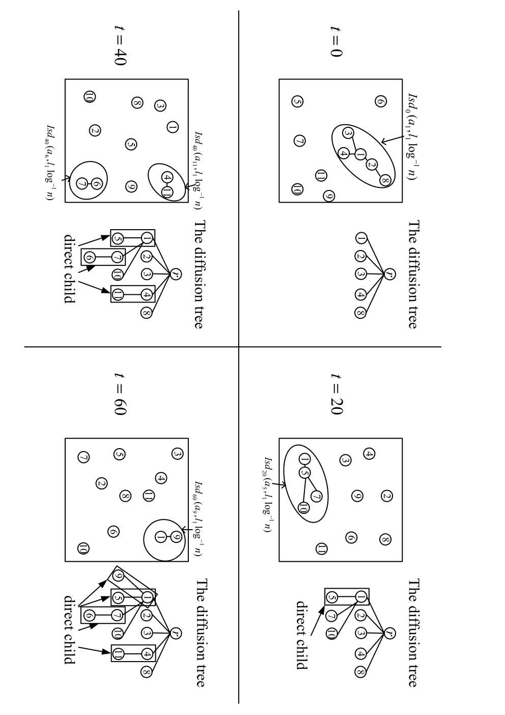
Refer to caption
Figure 1: An example of the diffusion process and its corresponding diffusion tree at t=0,20,40,60t=0,20,40,60. Assume no collisions happen beyond these 4 time steps.

  At t=0t=0, the agent a1\mathrm{a}_{1} is initially infected. Since Isd0​(a1,ℓ1​log−1​n)={a1,a2,a3,a4,a8}{\mathrm{Isd}}_{0}(\mathrm{a}_{1},\ell_{1}\log^{-1}n)=\{\mathrm{a}_{1},\mathrm{a}_{2},\mathrm{a}_{3},\mathrm{a}_{4},\mathrm{a}_{8}\}, the agents a2,a3\mathrm{a}_{2},\mathrm{a}_{3}, a4\mathrm{a}_{4}, and a8\mathrm{a}_{8} are all considered infected at t=0t=0. Also, 𝐫\mathbf{r} does not have a direct child.

  At t=20t=20, the agent a1\mathrm{a}_{1} meets a5\mathrm{a}_{5}. Since Isd20​(a1,ℓ1​log−1​n)={a1,a5,a7,a10}{\mathrm{Isd}}_{20}(\mathrm{a}_{1},\ell_{1}\log^{-1}n)=\{\mathrm{a}_{1},\mathrm{a}_{5},\mathrm{a}_{7},\mathrm{a}_{10}\}, a7\mathrm{a}_{7} and a10\mathrm{a}_{10} are also infected. At this time step, dchild⁡(a1)={a5}\mathrm{dchild}(\mathrm{a}_{1})=\{\mathrm{a}_{5}\} and child⁡(a1)={a5,a7,a10}{\mathrm{child}}(\mathrm{a}_{1})=\{\mathrm{a}_{5},\mathrm{a}_{7},\mathrm{a}_{10}\}.

  At t=40t=40, a4\mathrm{a}_{4} meets a11\mathrm{a}_{11} and a6\mathrm{a}_{6} meets a7\mathrm{a}_{7}; Isd40​(a4,ℓ1​log−1​n)={a4,a11}{\mathrm{Isd}}_{40}(\mathrm{a}_{4},\ell_{1}\log^{-1}n)=\{\mathrm{a}_{4},\mathrm{a}_{11}\} and Isd40​(a7,ℓ1​log−1​n)={a6,a7}{\mathrm{Isd}}_{40}(\mathrm{a}_{7},\ell_{1}\log^{-1}n)=\{\mathrm{a}_{6},\mathrm{a}_{7}\}. At this time step, child4​(a4)=dchild⁡(a4)={a11}{\mathrm{child}}_{4}(\mathrm{a}_{4})=\mathrm{dchild}(\mathrm{a}_{4})=\{\mathrm{a}_{11}\} and child⁡(a7)=dchild⁡(a7)={a6}{\mathrm{child}}(\mathrm{a}_{7})=\mathrm{dchild}(\mathrm{a}_{7})=\{\mathrm{a}_{6}\}. Notice that a11∈𝔽1\mathrm{a}_{11}\in\mathbb{F}_{1} and a6∈𝔽3\mathrm{a}_{6}\in\mathbb{F}_{3}. These two generations grow simultaneously at t=40t=40.

  At t=60t=60, a1\mathrm{a}_{1} meets a9\mathrm{a}_{9}. Isd60​(a9)={a1,a9}{\mathrm{Isd}}_{60}(\mathrm{a}_{9})=\{\mathrm{a}_{1},\mathrm{a}_{9}\}. We have a9∈child⁡(a1)\mathrm{a}_{9}\in{\mathrm{child}}(\mathrm{a}_{1}) and a9∈dchild⁡(a1)\mathrm{a}_{9}\in\mathrm{dchild}(\mathrm{a}_{1}). Also, notice that a1\mathrm{a}_{1} now contains two direct children.