The Lyman- $\alpha$ forest in three dimensions: measurements of large scale flux correlations from BOSS 1st-year data

Anže Slosar Affiliation: Brookhaven National Laboratory, Blgd 510, Upton NY 11375, USA Email: anze@bnl.gov Andreu Font-Ribera Affiliation: Institut de Ciències de l’Espai (CSIC-IEEC), Campus UAB, Fac. Ciències, torre C5 parell 2, Bellaterra, Catalonia Matthew M. Pieri Affiliation: Center for Astrophysics and Space Astronomy, University of Colorado, 389 UCB, Boulder, Colorado 80309, USA Affiliation: Department of Astronomy, Ohio State University, 140 West 18th Avenue, Columbus, OH 43210, USA James Rich Affiliation: CEA, Centre de Saclay, IRFU, 91191 Gif-sur-Yvette, France Jean-Marc Le Goff Affiliation: CEA, Centre de Saclay, IRFU, 91191 Gif-sur-Yvette, France Éric Aubourg Affiliation: CEA, Centre de Saclay, IRFU, 91191 Gif-sur-Yvette, France Affiliation: APC, Université Paris Diderot-Paris 7, CNRS/IN2P3, CEA, Observatoire de Paris, 10, rue A. Domon & L. Duquet, Paris, France Jon Brinkmann Affiliation: Apache Point Observatory, P.O. Box 59, Sunspot, NM 88349,USA Nicolas Busca Affiliation: APC, Université Paris Diderot-Paris 7, CNRS/IN2P3, CEA, Observatoire de Paris, 10, rue A. Domon & L. Duquet, Paris, France Bill Carithers Affiliation: Lawrence Berkeley National Laboratory, 1 Cyclotron Road, Berkeley, CA 94720, USA. Romain Charlassier Affiliation: CEA, Centre de Saclay, IRFU, 91191 Gif-sur-Yvette, France Marina Cortês Affiliation: Lawrence Berkeley National Laboratory, 1 Cyclotron Road, Berkeley, CA 94720, USA. Rupert Croft Affiliation: Bruce and Astrid McWilliams Center for Cosmology, Carnegie Mellon University, Pittsburgh, PA 15213, USA Kyle S. Dawson Affiliation: University of Utah, Dept. of Physics & Astronomy, 115 S 1400 E, Salt Lake City, UT 84112, USA Daniel Eisenstein Affiliation: Harvard College Observatory, 60 Garden St., Cambridge MA 02138, USA Jean-Christophe Hamilton Affiliation: APC, Université Paris Diderot-Paris 7, CNRS/IN2P3, CEA, Observatoire de Paris, 10, rue A. Domon & L. Duquet, Paris, France Shirley Ho Affiliation: Lawrence Berkeley National Laboratory, 1 Cyclotron Road, Berkeley, CA 94720, USA. Khee-Gan Lee Affiliation: Department of Astrophysical Sciences, Princeton University, Princeton, New Jersey 08544, USA Robert Lupton Affiliation: Department of Astrophysical Sciences, Princeton University, Princeton, New Jersey 08544, USA Patrick McDonald Affiliation: Brookhaven National Laboratory, Blgd 510, Upton NY 11375, USA Affiliation: Lawrence Berkeley National Laboratory, 1 Cyclotron Road, Berkeley, CA 94720, USA. Bumbarija Medolin Affiliation: 104-20 Queens Blvd #17A, Forest Hills, NY 11375, USA Jordi Miralda-Escudé Affiliation: Institució Catalana de Recerca i Estudis Avançats, Barcelona, Catalonia Affiliation: Institut de Ciències del Cosmos, Universitat de Barcelona/IEEC, Barcelona 08028, Catalonia Demitri Muna Affiliation: Center for Cosmology and Particle Physics, New York University, New York, NY 10003 USA Adam D. Myers Affiliation: Department of Astronomy, MC-221, University of Illinois, 1002 West Green Street, Urbana, IL 61801, USA Affiliation: Department of Physics and Astronomy, University of Wyoming, Laramie, WY 82071, USA Robert C. Nichol Affiliation: Institute of Cosmology and Gravitation (ICG), Dennis Sciama Building, Burnaby Road, Univ. of Portsmouth, Portsmouth, PO1 3FX, UK. Nathalie Palanque-Delabrouille Affiliation: CEA, Centre de Saclay, IRFU, 91191 Gif-sur-Yvette, France Isabelle Pâris Affiliation: Université Paris 6 et CNRS, Institut d’Astrophysique de Paris, 98bis blvd. Arago, 75014 Paris, France Patrick Petitjean Affiliation: Université Paris 6 et CNRS, Institut d’Astrophysique de Paris, 98bis blvd. Arago, 75014 Paris, France Yodovina Piškur Affiliation: Department of Astrophysical Sciences, Princeton University, Princeton, New Jersey 08544, USA Emmanuel Rollinde Affiliation: Université Paris 6 et CNRS, Institut d’Astrophysique de Paris, 98bis blvd. Arago, 75014 Paris, France Nicholas P. Ross Affiliation: Lawrence Berkeley National Laboratory, 1 Cyclotron Road, Berkeley, CA 94720, USA. David J. Schlegel Affiliation: Lawrence Berkeley National Laboratory, 1 Cyclotron Road, Berkeley, CA 94720, USA. Donald P. Schneider Affiliation: Department of Astronomy and Astrophysics, The Pennsylvania State University, 525 Davey Lab, University Park, PA 16802, USA Erin Sheldon Affiliation: Brookhaven National Laboratory, Blgd 510, Upton NY 11375, USA Benjamin A. Weaver Affiliation: Institució Catalana de Recerca i Estudis Avançats, Barcelona, Catalonia David H. Weinberg Affiliation: Department of Astronomy, Ohio State University, 140 West 18th Avenue, Columbus, OH 43210, USA Christophe Yeche Affiliation: CEA, Centre de Saclay, IRFU, 91191 Gif-sur-Yvette, France Donald G. York Affiliation: Department of Astronomy and Astrophysics, University of Chicago, 5640 South Ellis Avenue, Chicago, IL 60637, USA Affiliation: Enrico Fermi Institute, University of Chicago, 5640 South Ellis Avenue, Chicago, IL 60637, USA

Abstract

Using a sample of approximately 14,000 $z>2.1$ quasars observed in the first year of the Baryon Oscillation Spectroscopic Survey (BOSS), we measure the three-dimensional correlation function of absorption in the Lyman- $\alpha$ forest. The angle-averaged correlation function of transmitted flux ( $F=e^{-\tau}$ ) is securely detected out to comoving separations of $60\,h^{-1}\,{\rm Mpc}$ , the first detection of flux correlations across widely separated sightlines. A quadrupole distortion of the redshift-space correlation function by peculiar velocities, the signature of the gravitational instability origin of structure in the Lyman- $\alpha$ forest, is also detected at high significance. We obtain a good fit to the data assuming linear theory redshift-space distortion and linear bias of the transmitted flux, relative to the matter fluctuations of a standard $\Lambda$ CDM cosmological model (inflationary cold dark matter with a cosmological constant). At 95% confidence, we find a linear bias parameter $0.16<b<0.24$ and redshift-distortion parameter $0.44<\beta<1.20$ , at central redshift $z=2.25$ , with a well constrained combination $b~(1+\beta)=0.336\pm 0.012$ . The errors on $\beta$ are asymmetric, with $\beta=0$ excluded at over $5\sigma$ confidence level. The value of $\beta$ is somewhat low compared to theoretical predictions, and our tests on synthetic data suggest that it is depressed (relative to expectations for the Lyman- $\alpha$ forest alone) by the presence of high column density systems and metal line absorption. These results set the stage for cosmological parameter determinations from three-dimensional structure in the Lyman- $\alpha$ forest, including anticipated constraints on dark energy from baryon acoustic oscillations.

Keywords

cosmology, Lyman-

\alpha

forest, large scale structure, dark energy

1 Introduction

Early spectra of high-redshift ( $z>2$ ) quasars showed ubiquitous absorption lines blueward of their Lyman- $\alpha$ emission, which were identified as arising primarily from Lyman- $\alpha$ absorption by intervening concentrations of neutral hydrogen [1]. While early models described the absorbers as discrete clouds analogous to those in the interstellar medium, a combination of theoretical and observational advances in the mid-1990s led to a revised view of the forest as a continuous phenomenon, analogous to Gunn-Peterson [2] absorption but tracing an inhomogeneous, fluctuating intergalactic medium (see, e.g., the review by [3]). This revision of theoretical understanding also transformed the promise of the Lyman- $\alpha$ forest as a tool for cosmology, by showing that the forest traces the distribution of dark matter in the high-redshift universe in a relatively simple way. Adopting this “continuous medium” view, several groups [4, 5, 6, 7, 8, 9] measured the power spectrum of Lyman- $\alpha$ forest flux in successively larger samples of quasar spectra and used it to constrain the power spectrum of the underlying dark matter distribution. The most recent of these measurements [9], using a large quasar sample from the Sloan Digital Sky Survey (SDSS; [10, 11, 12, 13, 14, 15, 16, 17]), have provided some of the strongest constraints on inflation, neutrino masses, and the “coldness” of dark matter, especially when combined with data sets that probe other redshifts and/or physical scales (e.g., [18, 19, 20, 21, 22, 23]). However, while the underlying density field is three-dimensional, all of these cosmological analyses have treated the forest as a collection of independent 1-dimensional maps.

This paper presents measurements of Lyman- $\alpha$ forest flux correlations across parallel lines of sight with the widest separation reached so far, taking advantage of the large sample of high-redshift quasars observed during the first year of BOSS, the Baryon Oscillation Spectroscopic Survey of SDSS-III [24].

Measurements of correlated absorption towards gravitational lenses and closely separated quasar pairs [25, 26, 27, 28] provided some of the critical observational evidence for the revised understanding of the Lyman- $\alpha$ forest. These transverse correlation measurements implied a coherence scale of several hundred $\,h^{-1}\,{\rm kpc}$ (comoving) for individual absorbing structures. The large sizes and low neutral column densities in turn implied that the absorbing gas has low densities and is highly photoionized by the intergalactic UV background, making the total baryon content of the forest a large fraction of the baryons allowed by Big Bang nucleosynthesis [29]. Hydrodynamic cosmological simulations naturally explained these large coherence scales and many other statistical properties of the forest [30, 31, 32, 33], with typical absorption features arising in filamentary structures of moderate overdensity, $\delta\equiv\rho/\bar{\rho}-1\sim 20$ . Detailed investigation of these simulations revealed an approximate description of the forest that is both surprisingly simple and surprisingly accurate [34, 35]: the Lyman- $\alpha$ forest arises in gas that traces the underlying dark matter distribution, except for small scale pressure support, with the neutral hydrogen fraction determined by photoionization equilibrium, and with a power-law temperature-density relation $T\propto(\rho/\bar{\rho})^{\gamma-1}$ . This relation is established by the competition of photoionization heating and adiabatic cooling [36]. In this approximation, the transmitted flux fraction $F$ is related to the dark matter overdensity $\delta$ by

F=e^{-\tau}=\exp\left[-A(1+\delta)^{2-0.7(\gamma-1)}\right]~,

(1)

where the temperature-density slope $(\gamma-1)$ depends on the inter-galactic medium (IGM) reionization history, and the constant $A$ depends on redshift and on a variety of physical parameters (see [37] for a recent discussion). On large scales, the three-dimensional power spectrum of the field $\delta_{F}\equiv F/\bar{F}-1$ should have the same shape as the power spectrum of $\delta=\rho/\bar{\rho}-1$ [35, 4, 5]. Thermal motions of atoms smooth spectra on small scales, producing a turnover in the one-dimensional flux power spectrum at high $k$ . (In practice, peculiar velocities, which we discuss next, produce a turnover at larger scales than thermal motions.)

The most significant correction to equation (1) is from peculiar velocities, which shift the apparent locations of the absorbing neutral hydrogen in the radial direction. On large scales, the power spectrum should approximately follow the linear theory model of redshift-space distortions,

P_{F}(k,\mu_{k})=b^{2}P_{L}(k)(1+\beta\mu_{k}^{2})^{2}~,

(2)

where $P_{L}(k)$ is the real-space linear power spectrum and $\mu_{k}$ is the cosine of the angle between the wavevector ${\bf k}$ and the line of sight. The bias factor $b$ of the forest is the bias factor of the contrast of the flux fluctuations and not the bias factor of the neutral hydrogen. It is typically low because the full range of density variations is mapped into the transmitted flux range $0<F<1$ ( $b$ is actually technically negative, because overdensities in mass produce smaller $F$ , but this is irrelevant to our paper so we will just quote $|b|$ ). While the functional form in Eq. 2 is that of Kaiser [38], the parameter $\beta$ does not have the same interpretation, coming from a more general linear theory calculation of redshift-space distortions in the case where the directly distorted field, in this case optical depth, undergoes a subsequent non-linear transformation, in this case $F=\exp(-\tau)$ [5, 39]. For a galaxy survey, $\beta\approx[\Omega_{m}(z)]^{0.55}/b$ , but for the Lyman- $\alpha$ forest $\beta$ can vary independently of $\Omega_{m}$ and $b$ , i.e., it is generally a free parameter.

The simulations of [39] suggest an approximate value of $\beta\approx 1.47$ at $z\approx 2.25$ (interpolating over the parameter dependences in Table 1 of [39], since the central model there is antiquated). Lower resolution calculations of [40] ( $500h^{-1}{\rm kpc}$ mean particle spacing and particle-mesh (PM) cell size) found a lower value $\beta\sim 1$ . Unpublished work by Martin White demonstrates that the value of $\beta$ predicted by PM simulations with different smoothing applied to the mass density field decreases with increasing smoothing length (based simulations with $73~h^{-1}{\rm kpc}$ resolution, and in agreement with the $\sim 180~h^{-1}{\rm kpc}$ resolution simulation in [41]). Reference [39] concurred that low resolution simulations produce lower $\beta$ , and agree with White on the value at similar smoothing, so the fundamental outstanding question for predicting $\beta$ is apparently how smooth is the gas in the IGM ([39] quantifies other parameter dependences, but none of them make so much difference, given the relatively small uncertainty in those parameters, for vanilla models at least). The smoothing scale of the IGM is determined mostly by the pressure, i.e., Jeans smoothing, which is determined by the temperature history of the gas [42, 43]. A linear theory calculation of the smoothing scale for reasonable thermal history, following [42], predicts $\sim 100\,h^{-1}\,{\rm kpc}$ or slightly more (this is the rms smoothing length for a Gaussian kernel applied to the density field). [39] used the hydro-PM (HPM) approximation of [42] to include pressure in the non-linear evolution of otherwise PM simulations and found results consistent with smoothing PM by a smaller amount, $\sim 40\,h^{-1}\,{\rm kpc}$ . We know of no reason to doubt the qualitative accuracy of the HPM simulations, but ultimately fully hydrodynamic simulations will be required to decisively compute the expected value of $\beta$ for a given model. [44] plotted the 3D power spectrum from a hydro simulation, and suggested $\beta$ could be $\sim 1$ , but their single $25\,h^{-1}\,{\rm Mpc}$ simulation box had too few modes in the comfortably linear regime to assess the accuracy of this result. Finally, even if we were sure of our calculation for a given thermal history, there is some uncertainty due to uncertainty about the thermal history, especially the redshift of reionization (we have not quantified how large this uncertainty is).

Refer to caption — Figure 1: Survey area of the quasars used in this paper in equatorial coordinates, in the Aitoff projection.

Figure 3: Redshift distribution of quasars for the sample used in this analysis (left panel), and weighted distribution of Lyman-

\alpha

forest pixel redshifts for the three redshift bins considered in this paper (right panel). The quasar redshifts are cut to be between

2.1<z<3.5

. The pixel weights are limited by the UV coverage of the spectroscope at low redshift end and by the redshift of quasars at high redshift. We show the sample of quasars without DLA flag; however, the two plots are virtually identical for the sample in which DLA flagged quasars are included.

At the percent level needed to interpret 1D power spectrum measurements, the value of the bias parameter $b$ is well known to depend on the mean absorption level (shown directly in [39]), which is difficult to determine accurately; however, at the level of this paper it is actually quite precisely predicted, with [39] and [41] (verified by Martin White, private communication) agreeing on a value $\sim 0.13$ to $\sim 10$ % with less sensitivity to smoothing than for $\beta$ ([40] did find a higher value $\sim 0.18$ for their much lower $500h^{-1}{\rm kpc}$ resolution simulation).

In addition to quasar pair measurements, there have been some studies of closely spaced groupings of quasars that provide hints of three-dimensional structure in the Lyman- $\alpha$ forest [45, 46, 47, 48, 49, 50, 51, 52, 53]. However, large scale flux correlations are weak, so detecting them with high significance across widely separated sightlines requires a large and dense quasar sample. By design, the BOSS quasar survey provides precisely such a sample, probing a large comoving volume with $\sim 15$ sightlines per deg².

The ultimate goal of the BOSS survey is to measure the baryon acoustic oscillation (BAO) feature to high precision in the galaxy redshift survey at $z<0.7$ and Lyman- $\alpha$ forest at $z\approx 2.5$ [24] (the possibility of measuring the BAO feature using the Lyman- $\alpha$ forest was suggested in [39] and some preliminary calculations were done by [54], but the potential of the measurement was not really quantified until [55] (see also [40, 41, 56]). These measurements will be used as a standard ruler to measure the angular diameter distance $D_{A}(z)$ and Hubble parameter $H(z)$ . The first proof-of-concept paper for the galaxy part of the survey is [57], and this paper attempts to do the same for the Lyman- $\alpha$ forest part of the survey. The sample of 14,000 quasars analyzed in this paper is too small to yield a confident detection of the BAO feature, but it does allow the first precise measurements of three-dimensional structure in the Lyman- $\alpha$ forest. The basic statistic that we use is the flux correlation function

\xi_{F}(r,\mu)=\langle\delta_{F}({\bf x})\delta_{F}({\bf x}+{\bf r})\rangle~,

(3)

which is the Fourier transform of the power spectrum (2). Our measurements provide novel tests of the basic cosmological understanding of high-redshift structure and the nature of the Lyman- $\alpha$ forest.

The next section describes our data sample, based on quasars observed by BOSS between December 2009 and July 2010. During these first few months of BOSS, which included commissioning of new hardware, software, and observing procedures, data taking was relatively inefficient. Our sample of 14,598 $z>2.1$ quasars over $\sim 880$ square degrees is less than 10% of the anticipated final sample of 150,000 quasars selected over 10,000 deg², but it is already comparable to the total number of $z>2.1$ quasars found by SDSS-I and II [58]. Section 3 describes our methods for creating realistic synthetic data sets, which are crucial to testing our measurement and error estimation procedures and which we use as a source of theoretical predictions for comparison to our measurements. Section 4 describes our analysis procedures including removal of continuum, estimation of the flux correlation function and its statistical errors, and model fitting, presenting detailed tests of these procedures on the synthetic data. Section 5 presents the main results of the BOSS analysis. We describe several internal tests for systematic errors in §6, and we summarize our results in §7 with final remarks given §8.

2 Data sample

In this section we give a brief overview of the BOSS Quasar data sample that was used in our analysis, and the French Participation Group (FPG) visual inspections of the BOSS spectra. The quasar target selection for the first year of BOSS observations is described in detail in [59], which draws together the various methods presented in [60, 61] and [62]. In summary, selecting $z>2.1$ , and in particular $2.1<z<3.5$ objects, has always been challenging due to the colours of quasars at these redshifts crossing over the stellar locus in, e.g., SDSS ugriz optical colour-space [63]. Therefore, the “UV Excess” method, generally used for $z<2$ objects, fails. As such, the $2.2<z<3.5$ redshift range was sparsely sampled in the original SDSS, and the number density of $z>3.5$ objects was very low ( $\sim$ few deg^-2).

In BOSS, selecting $2.2<z<3.5$ is key to meeting our science requirements. We have the advantage that when one selects the quasars only as backlights for the detection of neutral hydrogen, one is at liberty to use a combination of methods to select quasars without having to understand the completeness of the sample in any variable relevant for studying quasar properties or clustering. In total 54,909 spectra were taken by BOSS that were targeted as high, $z>2.2$ , quasar targets between Modified Julian Dates (MJDs) 55176 (11 Dec 2009) and 55383 (6 July 2010). From this sample, 52,238 are unique objects, and have SDSS PSF magnitudes in the range $18.0<r<22.0$ . Of these 52,238 objects, 13,580 (14,810) quasars have $z\geq 2.20\ (2.10)$ and a secure redshift as given by the BOSS spectro-pipeline.

Although the BOSS spectro-pipeline is secure at the 90-95% level, a non-negligible number of objects are classified as QSOs when they are stars and vice-versa. Because of this, the nearly 55,000 objects were also visually inspected by one, or more, of the BOSS team members. These inspections are generally referred to as the FPG inspections. The manual inspections of the BOSS spectra give a further level of confidence in the data, and result in a net gain of real high- $z$ quasars that the pipeline does not select, at the level of $\sim 1-3$ objects per 7 deg² plate. Moreover, the visual inspection has the option to manually label high- $z$ quasars which have either Damped Lyman- $\alpha$ (DLA) or Broad Absorption Line (BAL) features. Currently, this option is binary in the sense that the visual inspector has the option of setting the BAL and DLA flags but no attempt is made to measure $N_{\rm HI}$ column density or the position of the absorber. We have checked that the flagged DLAs have log $N$ (H i)(cm^-2) $>\sim 20.3$ . The list is not complete however, since DLAs are difficult to detect along lines of sight of SNR $<$ 4 [64]. We have also checked that the so-called balnicity index is larger than 2000 km s^-1 (see e.g. [65]). The removal of DLA systems in our data hence still depends on a human factor and signal-to-noise ratio and is currently not a very well quantified process. This will become better defined in future work.

For the analysis presented here, those objects labeled by the FPG visual inspections as “BAL” are not used, and we don’t include objects labeled as “DLA” unless mentioned specifically.

In our sample we restrict the analysis to quasars from the FPG sample with $2.1<z<3.5$ . Compared to the targeted science sample described above, this sample has no magnitude cut, expands the lower redshift to $z=2.1$ and uses some quasars that are on plates nominally marked as “bad” by the pipeline, but contain useful data based on manual inspections. After removing approximately 1300 quasars marked as BALs, our complete sample contains 14,598 quasars, of which 13,743 are not labeled as having a DLA. Several quasars in the first year sample had repeated observations - we do not use these repeats and limit ourselves to the best quality observation (as determined by FPG). The FPG visual inspections are continuously being updated and revised. We froze the data used on 1^st October 2010.

Further details about the target selection and details about the instrument and the observational procedure can be found in [59].

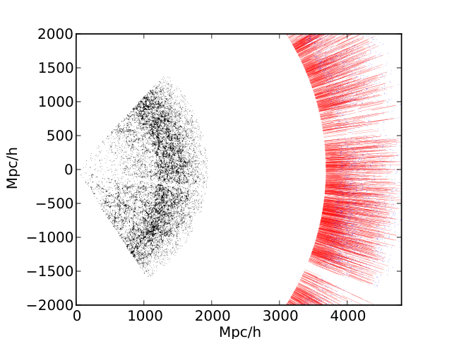
Figure 1 shows the position of the BOSS Year One quasars on the sky in equatorial projections in the Aitoff projection. Figure 2 shows the geometry of BOSS probes of large scale structure in comoving coordinates. Figure 3 gives the redshift distribution of the $z>2.1$ quasars and the weighted histogram of pixel redshifts contributing to our correlation measurement (explained and discussed later), as a function of redshift.

3 Synthetic data

To test our data reduction pipeline and to examine the impact of various systematics, we created extensive synthetic datasets. These synthetic data shared the geometry with the observed set of quasars, i.e. the positions and redshifts of quasars were identical, and we used the observed SDSS $g$ magnitudes to normalize the spectra.

The statistical properties of synthetic data matched our initial estimate of the properties of the underlying flux field, including the non-linear corrections to the linear redshift-space distortions [39].

The Lyman- $\alpha$ absorption spectra of each quasar were generated using a method described below to obtain the variable $\delta_{F}=F/\bar{F}-1$ , where $F$ is the fraction of transmitted flux, at each spectral pixel from a realization of the underlying cosmological density fluctuations, including linear redshift-space distortions and non-linear corrections to the flux power spectrum model that is used as input. A total of 30 different realizations of this underlying cosmological field were generated. For each realization, the following sets of synthetic data were created, with increasing level of realism to evaluate the impact of various observational effects and of our data reduction procedure:

•

Noiseless measurements of $\delta_{F}$
•

Noiseless measurements of Lyman- $\alpha$ forest with continua
•

Noisy measurements of Lyman- $\alpha$ forest with continua
•

Noisy measurements of Lyman- $\alpha$ forest with continua and high-absorption systems
•

Noisy measurements of Lyman- $\alpha$ forest with continua and forest metal contamination
•

Noisy measurements of Lyman- $\alpha$ forest with continua and forest metal contamination and high-absorption systems

Note that continua here means variable continua using randomly generated PCA eigenmode amplitudes [66], instead of the same mean continuum for every QSO.

In the following subsections we briefly describe how these synthetic data are actually generated. The generation of Lyman- $\alpha$ absorption and associated structure will be discussed in more detail in [67].

3.1 Absorption field

3.1.1 Generation of a Gaussian field

A Lyman- $\alpha$ forest survey samples the intrinsically three-dimensional flux transmission fraction field along a set of infinitesimally thin lines of sight to quasars. The brute force method for generating a survey with correct correlations would be to generate the full 3D field with sufficient resolution (tens of kpc), and then read off the density along lines of sight. For a survey as large as ours, this requires too much memory. Fortunately, when generating a Gaussian field we can greatly simplify the problem, maintaining exact high-resolution statistics while only creating the field for the limited fraction of the volume where it is required.

To generate a Gaussian random field for a general set of pixels with covariance matrix $\mathbf{C}$ we can Cholesky decompose the covariance matrix, i.e. first find $\mathbf{L}$ such that

\mathbf{L}\cdot\mathbf{L}^{T}=\mathbf{C}.

(4)

If we then generate a unit variance white noise field $w_{j}$ in the pixels and multiply it by $L_{ij}$ , the resulting field will have the desired correlation function, i.e.

\left<\delta_{i}\delta_{j}\right>=\left<L_{ik}w_{k}L_{jl}w_{l}\right>=L_{ik}L^{T}_{kj}=C_{ij}.

(5)

Assuming the lines of sight are parallel allows another significant simplification. Suppose the field $\delta\left(x_{\parallel},\mathbf{x_{\perp}}\right)$ has power spectrum $P\left(k_{\parallel},k_{\perp}\right)$ . If we Fourier transform this field in the radial direction only, the resulting modes have correlation

\left<\delta\left(k_{\parallel},\mathbf{x_{\perp}}\right)\delta\left(k_{\parallel}^{\prime},\mathbf{x_{\perp}}^{\prime}\right)\right>=2\pi~\delta^{D}\left(k_{\parallel}+k_{\parallel}^{\prime}\right)P_{\times}\left(k_{\parallel},\left|\mathbf{x_{\perp}}-\mathbf{x_{\perp}}^{\prime}\right|\right)~,

(6)

where

P_{\times}\left(k_{\parallel},r_{\perp}\right)=\frac{1}{2\pi}\int_{k_{\parallel}}^{\infty}k~dk~J_{0}\left(k_{\perp}r_{\perp}\right)~P\left(k,\mu_{k}\right)~,

(7)

where $k_{\perp}=\sqrt{k^{2}-k_{\parallel}^{2}}$ and $\mu_{k}=k_{\parallel}/k$ . The key point is that modes with different values of $k_{\parallel}$ are uncorrelated. We can generate the field efficiently by following the above general procedure for generating a correlated Gaussian random field, except now independently for every value of $k_{\parallel}$ required for the radial Fourier transform. We never need to manipulate a matrix larger than a manageable $N_{q}\times N_{q}$ , where $N_{q}$ is the number of quasars. However, we do take into account the fact that lines of sight are not fully parallel as discussed in Section 3.1.3.

We use this procedure to generate any desired Gaussian field $\delta$ at each pixel of each quasar spectrum of the synthetic data sets, once we have a model for the power spectrum $P(k,\mu_{k})$ of this variable.

3.1.2 Generation of the transmitted flux fraction, $F$

In order to obtain realistic synthetic data including noise as in the observed spectra, it is necessary to generate the flux transmission fraction $F$ with a realistic distribution in the range $0$ to $1$ , and add the noise to this flux variable. The solution we have adopted is to convert the Gaussian fields $\delta$ to a new field $F(\delta)$ with any desired distribution. In this paper we use a log-normal distribution in the optical depth, $\tau=-\log F$ (where log denotes natural logarithm), which implies the following probability distribution for $F$ :

p(F)\,dF={\exp\left[-(\log\tau-\log\tau_{0})^{2}/(2\sigma_{\tau}^{2})\right]\over\tau F\sqrt{2\pi}\sigma_{\tau}}\,dF~,

(8)

with the two parameters $\tau_{0}$ and $\sigma_{\tau}$ that determine the mean and dispersion of $F$ . We find the function $F(\delta)$ that results in this distribution for $F$ when $\delta$ is a Gaussian variable. The correlation function of the variables $\delta$ and $F$ are then related by the following equation:

$\displaystyle\xi_{F}(r_{12})=$	$\displaystyle\left<F_{1}F_{2}\right>$
$\displaystyle=$	$\displaystyle\int_{0}^{1}dF_{1}\int_{0}^{1}dF_{2}p(F_{1},F_{2})F_{1}F_{2}$
$\displaystyle=$	$\displaystyle\int_{-\infty}^{\infty}d\delta_{1}\int_{-\infty}^{\infty}d\delta_{2}p(\delta_{1},\delta_{2})F_{1}F_{2}$
$\displaystyle=$	$\displaystyle\int_{-\infty}^{\infty}d\delta_{1}\int_{-\infty}^{\infty}d\delta_{2}\frac{e^{-\frac{\delta_{1}^{2}+\delta_{2}^{2}-2\delta_{1}\delta_{2}\xi^{2}(r_{12})}{2(1-\xi^{2}(r_{12}))}}}{2\pi\sqrt{1-\xi^{2}(r_{12})}}F(\delta_{1})F(\delta_{2})~.$	(9)

We note that this equation relates $\xi_{F}$ to $\xi$ , independently of the variables $r$ , $\mu$ and $z$ . Therefore, we simply tabulate $\xi_{F}(\xi)$ , and invert the relation to figure out the correlation function $\xi$ that is required in order to obtain any desired correlation function $\xi_{F}$ .

We use a model for the flux power spectrum in redshift space, $P_{F}(k,\mu_{k})$ , which was fitted to the results of simulations in [39]. We use the value of $\beta$ for the central model in that paper, $\beta=1.58$ , and a bias inspired by the central model but roughly adjusted for cosmological model (not using the parameter dependence Table in [39]), $b=0.145$ , at $z=2.25$ . When generating the synthetic data, we keep the value of $\beta$ constant as a function of redshift, and vary the amplitude of the power spectrum according to a power-law, $P_{F}\propto(1+z)^{\alpha}$ . We compute the correlation function $\xi_{F}$ from the Fourier transform, then we calculate $\xi$ for the Gaussian field, and we Fourier transform back to obtain the desired power spectrum for $\delta$ . We generate this Gaussian field in all the quasar spectra with the method described above, and then transform this to the variable $\delta_{F}$ . In this way we obtain a set of spectra with the desired flux distribution and redshift-space power spectrum.

We use mean transmission fraction approximately matching the observations [8]: $\ln\left<F\right>(z)=\ln(0.8)\left[\left(1+z\right)/3.25\right]^{3.2}$ .

3.1.3 Redshift evolution and non-parallel lines of sight

The field $\delta_{F}$ is generated as described at a fixed redshift, and assuming parallel lines of sight. This is done at four different values of the redshift, by generating the realizations of the field with fixed random numbers for all the Fourier modes, and changing the amplitudes according to the different power spectra at every redshift. The power spectrum varies both because of the intrinsic evolution, and because the angular diameter distance used to convert angular to physical separation between the quasars varies with redshift. In this way, the fact that the lines of sight are non-parallel is incorporated into the calculation in the same way as the redshift evolution of the power spectrum. The final field $\delta_{F}$ is obtained by interpolating between the fields that have been generated at different redshifts, to the exact redshift of each point on the line of sight. This field then has the desired local power spectrum at any redshift, evolving as it is prescribed according to the linear interpolation.

The redshift evolution of amplitude assumed in this work is described by a power law $(1+z)^{\alpha}$ , with $\alpha=3.9$ as suggested by the measured evolution of the 1D flux power spectrum [9].

3.2 Adding absorption systems: Lyman Limit Systems (LLS) and Damped Lyman- $\alpha$ (DLA) systems

The highest column density absorption systems produce broad damped absorption wings which can have a strong impact on the correlation function of the transmitted flux. These systems are traditionally known as Damped Lyman Alpha absorbers (DLA) and have H I column densities above $10^{20.3}{\rm cm}^{-2}$ , however, the damping wings can affect the line profile at lower column densities as well. Systems with column densities above $10^{17.2}{\rm cm}^{-2}$ are known as Lyman Limit Systems (LLS) since they are self-shielded [68]. At $10^{17.2}{\rm cm}^{-2}$ , the effect of damping wings on the profile is small, but it becomes significant well before $10^{20.3}{\rm cm}^{-2}$ [69].

The impact of these absorption systems is two-fold. First, they add noise to the measurement of the correlation function. Second, the systems trace the underlying mass density field, and therefore they are correlated with themselves and with the Lyman- $\alpha$ absorption arising from the intergalactic medium. This systematically modifies the overall Lyman- $\alpha$ transmission correlation function.

To simulate the effect of these systems in the synthetic data, we introduce lines with $N_{\rm HI}>10^{17.2}{\rm cm}^{2}$ with an abundance consistent with observational constraints [70, 71, 72], using the formula of [69]. The decrease in $\left<F\right>(z=2.25)$ due to these systems is 0.014. We also introduce a correlation between these systems and the rest of the Lyman- $\alpha$ absorption by placing them only in regions where the optical depth is above a critical value $\tau_{0}$ , such that the probability of $\tau>\tau_{0}$ is 1%. This is performed to explore the way that the damped absorbers may bias the measured correlation function, but their detailed impact depends on the specifics of this correlation. We leave for a future analysis a better modeling of the cross-correlation of damped absorbers and the Lyman- $\alpha$ forest.

In the rest of the paper we refer to these contaminants as LLS/DLA.

3.3 Adding forest metal contamination

Absorption by intergalactic metals imprints correlated signal in quasar spectra on characteristic scales. These scales are set by the wavelength ratios of metal line transitions with Lyman- $\alpha$ and with each other. As a result, this correlated signal is a potential contaminant of large-scale structure measurements in the forest. In order to add forest metal absorption to the synthetic data we measure the strength of metals. We do this in a self-consistent manner by measuring metal line absorption in the continuum normalized BOSS Year One spectra (excluding spectra with known DLAs). We use a modified version of the method set out by [73] and measure these lines by stacking absorption lines between 1041Å–1185Å in the quasar rest-frame. We measure the signal associated with metal lines correlated with Lyman- $\alpha$ or Si III in the forest. This is described in Appendix C, including a look-up table of flux decrements measured in the composite spectra.

We introduce these metal absorption features to the full suite of mock data with no noise and no LLS/DLAs, on a pixel-by-pixel basis; we walk through the spectra and lower the transmitted flux by values from interpolation of this table, and then add Gaussian noise. As a result, we lower the mean transmitted flux by 0.003 in the mocks. This approach assumes that metal lines trace Lyman- $\alpha$ structure monotonically, and as such these 1D correlations will add metal structure to our 3D analysis. Full line profiles are recovered by virtue of our easing of the local minimum requirement (metal absorption is added at the wings of Lyman- $\alpha$ profiles as well as the center).

This technique does not provide a full description of metal absorption and, in particular, neglects the impact of scatter in metallicity and metal complexes. We test these mocks by stacking them in the same manner used for the BOSS Year One spectra. The metal correlations imprinted in the noise-free mocks are reasonably well recovered in these composite spectra. Composite spectra of the mocks with noise added (after metals have been introduced) show metal correlations that, where measurable, are up to 10% weaker than those seen in the observed data or added to the mocks in all cases except the Si III line seen in the strongest bin which is 30% weaker. This is caused by a combination of Gaussian noise and the probability distribution function of the flux. The noise distribution is symmetrical but, in the relevant regime, there are always far more pixels in the higher flux bin, which have weaker associated metal absorption. We conclude that metals added are probably an underestimate of the average metal absorption associated with Lyman- $\alpha$ lines, but these results are sufficient for an exploration of the approximate impact of forest metals. It seems unlikely that LLS/DLA interlopers are able to produce the observed metal signal for the reasons given in [73], however, we shall explore this issue further in future publications. We also combine forest metals with LLS/DLA corrected mocks by introducing these high column lines after forest metals have been added. Hence only metals associated with the Lyman- $\alpha$ forest are included.

3.4 Generating the spectra

Once we have created an absorption field for every line of sight, we proceed to generate the actual spectrum for each quasar, multiplying it by the “continuum” of the quasar, i.e. the unabsorbed spectrum.

We generate each quasar continuum shape taking into account the quasar redshift and using a mean rest-frame continuum and random PCA components derived from the low-redshift Hubble data [66]. The continuum is then normalized using the $g$ magnitude of the quasar (taking into account the Lyman- $\alpha$ forest absorption).

Since our data are sampled on precisely the same grid as the observed data, we can also introduce noise by using the actual values of noise from the observed data. We assume noise to be Gaussian with the absolute flux variance given by the pipeline, i.e., we do not correct the signal-to-noise ratio for differences between our randomly generated continuum level and the data level.

Because the mocks were generated before the data analysis procedure was finalized, we have mocks only for quasars with redshift $>2.2$ , while the data analysis uses $z_{q}>2.1$ .

4 Data analysis

In this section we describe the analysis applied to both real and synthetic data. Briefly, the steps involved in this analysis start with co-adding the multiple spectra of each quasar. We then fit a model for the mean quasar continuum and mean absorption from the whole set of spectra. This is used to determine the fluctuation in the fraction of transmitted flux, $\delta_{F}$ , from the observed flux, in each individual spectrum over the Lyman- $\alpha$ forest range. The correlation function is then measured from these flux fluctuations. The information on the distribution of datapoint pairs and the measured correlations feed into the code that estimates the errors on our correlation function. With the estimated correlation function and error-covariance matrix, we finally proceed to estimate the parameters in our model of the correlation function, in particular the two bias parameters. The next subsections explain in detail each of these steps.

4.1 Preparing the data

All spectra in this analysis were obtained with the BOSS spectrograph on the Sloan 2.5-meter telescope at Apache Point Observatory [15]. The BOSS instrument follows the design of the spectrograph previously used in SDSS, but with improved throughput, wider wavelength coverage, reduced sky background from smaller fibers and a larger number of fibers. A full description of the instrument will be reported in a future paper [74].

Observations are performed using 15-minute exposures that are processed immediately with a simple data reduction package. These quick reductions provide estimates of data quality that are evaluated by a pair of observers at APO to insure roughly uniform depth over the full survey. The observers cease exposures when estimates of the accumulated SNR exceed a minimum threshold, leading to an average exposure time of approximately 75 minutes per plate. Within 24 hours of completing a night of observations, the images are fully reduced into wavelength-calibrated, flux-calibrated, one dimensional spectra. Adapted from the SDSS-I/II spectroscopic reduction pipeline, version v5_4_14 of the BOSS pipeline is used to generate the spectra in this analysis. An updated version of the BOSS pipeline [75] is used for the first two years of spectra that will be publicly released in July, 2012.

The modeling of the noise associated with the flux measured at each wavelength is particularly important for measurements of correlated Lyman- $\alpha$ absorption. Noise is characterized for each pixel in the raw images early in the Spectro-2D stage of the BOSS data reduction pipeline. After bias removal, the flux in each pixel is converted from analog digital units into photon counts using CCD amplifier gains that were determined independently during the commissioning of the instrument. We generate a corresponding image to represent the variance by taking the sum of square of the readnoise (measured in the overscan region of each quadrant) and the gain-corrected flux measured at each pixel for which the flux is positive. Pixels that fluctuate to negative flux values are assigned a variance from the readnoise only. The relative pixel-to-pixel response in the data is corrected with a flat-field image and the variance for each pixel is rescaled accordingly. For each pixel, we then invert the variance into units of inverse variance, and set the inverse variance equal to zero for all pixels that are contaminated by cosmic rays or known cosmetic defects.

We transform each two-dimensional image into a set of one-dimensional spectra with an optimal extraction [76]. The flat-field exposure is used to determine the shape of the profile and the fiber-to-fiber variations in throughput. The arc lamp image is used to determine the wavelength solution, with linear corrections made in each exposure to match sky line locations. The profile is fit to each spectrum in the two-dimensional image weighted by the inverse variance. Each extracted spectrum and corresponding inverse variance vector are corrected to ensure a uniform response curve as determined from the fiber-to-fiber variations in throughput mentioned above. All corrections to the inverse variance and flux vector preserve the SNR for each pixel. Sky subtraction is performed on each individual exposure using a model for background that varies with fiber position. The model is determined from the one-dimensional spectra extracted from fibers that were intentionally set to regions where no objects had been detected in the SDSS imaging program. The inverse variance of all fibers is rescaled by a factor to force the error distribution of all sky fibers at each wavelength to have a normal distribution with unit variance. In the Lyman-alpha region of the spectra, this typically scales the errors by a factor of 1.1, and this scaling is never allowed to decrease the errors. This effectively corrects for systematic uncertainties in the sky modeling and subtraction. We also mask spectra around bright atmospheric emission lines, such as Hg (5460Å) and O I (5577Å).

At the final step in the Spectro-2D stage of the BOSS reduction pipeline, the spectra derived from individual exposures are combined into a coadded spectrum for each fiber. The Spectro-1D pipeline spectroscopically classifies and assigns redshifts to each object based upon a minimum chi-squared fit to a library of PCA templates derived from BOSS data.

In this analysis, we use the spectra output from the Spectro-2D pipeline before the coaddition. Instead of using the resampled coadds from Spectro-2D, we co-add the data using the same fixed wavelength grid as the pipeline, but combining the flux values of the closest pixels in wavelength from the individual exposures. This ensures, in the simplest possible way, that the noise of the co-added data is independent from pixel to pixel, at the expense of a poor treatment of the small scale fluctuations in the data. Since we are interested in large-scale correlations, we are not concerned about these effects. In each pixel the data are coadded using inverse variance weighting. We apply a small correction to the final variance in each pixel, which typically increases it by less than 10%, to ensure that the inter-exposure variance in pixels is consistent with the noise predicted by the pipeline for individual exposures.

Typical values of observational parameters for BOSS quasars used in this work can be found in the Table 1. An example of a BOSS spectrum after this reduction is shown in Figure 4. This spectrum has a somewhat higher than typical SNR of quasars in our sample.

Parameter	Value
Total number of QSOs	14,598 ( $\sim$ 160,000 in the complete survey)
QSO sky density	10-25 deg^-2 (typically $\sim$ 15 deg^-2)
QSO redshift range	2.2 - 3.5
Spectral resolution	$\sim 2.5{\rm\AA}\sim 2.5h^{-1}{\rm Mpc}$
Pixel scale	$\sim 1.0{\rm\AA}\sim 1.0h^{-1}{\rm Mpc}$
Signal to noise ratio per pixel	0.5 - 10 (typically $\sim$ 1)
Exposure times	Until SNR thresholds is reached, typically 5 $\times$ 15 minutes
g-band magnitude	18-22 (typically $\sim 21$ )

Table 1: Typical observational parameters for BOSS quasars

Figure 4: A quasar spectrum at redshift

z=3.276

from the first year of BOSS data. The Lyman-

\alpha

forest is the shaded region between the Lyman-

\alpha

and the Lyman-

\beta

emission lines. Other strong emission lines are also indicated.

4.2 Continuum fitting

The next step in analyzing the data is to fit the continuum. Our model for the flux measured at wavelength $\lambda$ in quasar $i$ at redshift $z_{i}$ is as follows:

f(\lambda,i)=a_{i}\,[\lambda_{r}/(1185{\,\rm\AA})]^{b_{i}}\,C(\lambda_{r})\bar{F}(\lambda)\left[1+\delta_{F}(\lambda,i)\right]~,

(10)

where $\lambda_{r}=\lambda/(1+z_{i})$ is the rest-frame wavelength. The term $C(\lambda_{r})$ denotes the mean rest-frame quasar spectrum, which is multiplied by a power law $a_{i}[\lambda/(1185\,{\rm\AA})]^{b_{i}}$ , where $a_{i}$ and $b_{i}$ are two parameters determined for each individual quasar. The power-law is included to allow for large-scale spectro-photometric errors that are present due to imperfect sky subtraction and calibration, as well as for any intrinsic variation in the quasar spectra. The term $\bar{F}(z)$ describes the mean absorption in the forest as a function of redshift. The entire product $a_{i}\lambda^{b_{i}}C(\lambda/(1+z_{q}))\bar{F}(z)$ is a well constrained quantity, but individual terms are correlated. For example, we can multiply $a_{i}$ and $\bar{F}(z)$ by a certain factor and absorb it into $C(\lambda/(1+z_{q}))$ ; this is also true for the power-law parameter $b_{i}$ . Consequently, some quantities ( $\bar{F}$ , $a_{i}$ , etc.) are determined only up to an overall normalization constant.

For the purpose of determining our fit to the mean quasar continuum and mean transmission, and the parameters $a_{i}$ and $b_{i}$ , we calculate an overall likelihood of all the data without taking into account the correlations of the forest and the continuum fluctuations in different spectral pixels. This simplification allows us to write this simple expression for the likelihood function,

\log\mathcal{L}=\sum_{i}\sum_{\lambda}\left[-\frac{\left[f(\lambda,i)-a_{i}[\lambda_{r}/(1185\,{\rm\AA})]^{b_{i}}\,C(\lambda_{r})\bar{F}(z)\right]^{2}}{2\sigma^{2}(i,\lambda)}-\log\sigma(i,\lambda)\right]+{\rm const.}.

(11)

Here, $\sigma(i,\lambda)$ is the sum of the variances due to measurement noise and the intrinsic variance, i.e., it contains both variance due to continuum errors as well a variance due to small scale flux fluctuations. This quantity is required to be a function of the observed wavelength only in the region of the Lyman- $\alpha$ forest (or equivalently, the Lyman- $\alpha$ forest redshift), while outside the forest we force it to depend only on rest-frame wavelength, which implicitly assumes that the dominant source of variation in that region is continuum errors. We do not necessarily believe his assumption is true, but this allows in one sense optimal weighting of different parts of the quasar spectrum outside the forest, i.e., prevents certain high-variance parts of the rest-frame spectrum from excessively affecting the solution. In the long term, this assumption will have to be relaxed.

We restrict the rest-frame wavelength range used for this fit between $1041\,$ Å and $1600\,$ Å, and we also discard the data at an observed wavelength bluer than $3600\,$ Å. We parameterize $C(\lambda_{r})$ using 20 equally-spaced spline nodes inside the forest ( $1041\,$ Å to $1185\,$ Å), and 20 equally-spaced spline nodes outside the forest ( $1185\,$ Å to $1600\,$ Å), with one point fixed to the center of the Lyman- $\alpha$ emission line. We also use 8 spline nodes in redshift for the mean transmission fraction $\bar{F}$ , another 8 spline nodes to describe the scatter in the forest as a function of redshift, and another 20 spline nodes to describe the rms variations with rest-frame wavelength outside the forest. The full model used in continuum fitting is therefore described by 76 global parameters and 2 parameters for each quasar, $a_{i}$ and $b_{i}$ .

Since we are completely ignoring the correlations between pixels, the numerical values of $\sigma^{2}(i,\lambda)$ and $\chi^{2}=-2\log\mathcal{L}$ have no physical interpretation. They should be thought of as merely assisting the fit to naturally incorporate the variances in the data. Therefore, it is not crucial that $\sigma^{2}$ is parameterized by redshift inside the forest and rest-wavelength outside. A possible criticism of our fitting procedure is that redward of the Lyman-alpha emission, 20 nodes of the spline fit are not enough to resolve the full structure of the mean continuum at the resolution of the BOSS spectrograph. However, these points are used only to assist with determining the values of $a_{i}$ and $b_{i}$ (the normalization and power law slope, relative to a mean continuum), and hence our determination of continuum must be only good enough to broadly describe the shape in that region.

We determine all the parameters using a specially crafted Markov Chain Monte Carlo (MCMC, see e.g. [77]) procedure to find the maximum of $\mathcal{L}$ . The global parameters are first varied, while keeping $a_{i}$ and $b_{i}$ fixed, taking several hundred accepted samples (steps in the chain) of the MCMC. Next, the global parameters are fixed and we vary just $a_{i}$ and $b_{i}$ for one quasar at a time, looping over all quasars. At this step, only the model for the particular quasar under consideration matters, and hence likelihood evaluations are extremely fast. We then go back to varying the global parameters and repeat the process for several accepted samples. This is iterated about 50 times (we have tested that using just 20 iterations negligibly affects the final results), and we finally take the sample with the optimal fit. The proposal function of the MCMC process learns the degeneracy directions by using the covariance of previously accepted samples, separately for the global parameters and the quasar-specific parameters. This MCMC process is simply used here as a functional maximizer, i.e., we take just the most likely sample. The process takes about 36 hours on an 8-core workstation.

4.3 Determination of $\delta_{F}$

The next step is determining the flux variation $\delta_{F}$ , reducing the resolution of our data and determining the weighting factors that are used for calculating the correlation function. First, the continuum is predicted at each pixel of each quasar spectrum. Then the observed flux and continuum are averaged over four consecutive pixels, weighted with the inverse variance. This provides coarser pixels and an estimate of the noise on the value of flux in each rebinned pixel, with a reduced resolution. The typical length of these rebinned pixels is $\sim 3h^{-1}{\rm Mpc}$ . We assume that the total variance in a coarse pixel is the sum of the noise plus the intrinsic variance in the flux field, which is a function of redshift. We then iteratively determine:

•

The intrinsic variance in the rebinned pixels, determined as a function of redshift by splining over 8 points in redshift.
•

A factor by which we multiply our estimate of the continuum in each quasar, which ensures that the flux averaged over the entire Lyman- $\alpha$ forest of the quasar equals the mean continuum averaged over the same interval. This average is calculated by weighting with the inverse total variance in each pixel.

We find that by forcing the average mean flux over the quasar forest to match that of the average continuum, we decrease the variance in the correlation function estimate, although we also erase all modes along the line of sight of wavelength larger than that of the size of the forest. The way that this elimination of the mean flux variation in each quasar alters the measured correlation function can be easily modeled, as discussed in Appendix A. The upshot is that we can correct the predicted correlation function for this effect using a simple theory with one parameter $\Delta r$ , which is the effective Lyman- $\alpha$ forest length. In the limit of $\Delta r\rightarrow\infty$ , the correction disappears, as expected. The value of $\Delta r$ can be predicted from first principles, but we let it be a nuisance parameter as explained later.

Finally, we find the average value of the fluctuation $\delta_{F}$ at each fixed observed wavelength by averaging over all quasars, and we then subtract this average from all the values of $\delta_{F}$ in each individual quasar. The average is calculated in wavelength intervals $\Delta\lambda/\lambda_{Ly\alpha\ }=0.001$ . This procedure, which removes purely radial modes, helps remove some systematics of imperfect sky subtraction or Galactic CaII absorption [78] that occur at a fixed wavelength. The analysis of synthetic data demonstrates that this negligibly impacts the measured Lyman- $\alpha$ correlation properties. Finally, we make a cut on pixels in $\delta_{F}$ that are over $6-\sigma$ away from zero in terms of the total variance. A handful of pixels were removed that way, but this cut makes negligible change in the resulting correlation function.

4.4 Estimation of the correlation function and its errors

We use the trivial sub-optimal estimator of the correlation function as simply the weighted average over pixel pairs,

\bar{\xi_{F}}(r,\mu)=\frac{\sum_{{\rm pairs}\ i,j}w_{i}w_{j}\,\delta_{Fi}\delta_{Fj}}{\sum_{{\rm pairs}\ i,j}w_{i}w_{j}},

(12)

where the weights $w_{i}$ are the total inverse variance (from both the measurement noise as well as the intrinsic variance due to small scale fluctuations in the forest). This estimator effectively assumes that the covariance matrix of the $\delta_{Fi}$ values can be approximated as diagonal. By construction it is an unbiased estimator, but it is not an optimal one. To avoid introducing contamination from the correlated residuals from continuum fitting errors, we include only pairs of points from different quasars when measuring the three-dimensional correlation function. We also measure the one-dimensional correlation function along each quasar, which is, however, only used for the error estimation.

Throughout we neglect signal-noise correlations that arise due to the fact that the Poisson noise associated with counting of the photons hitting the CCD is measured from the observed photon count rather than the underlying (and unknown) true expectation value of photon count. In [9] it was found that this results in 1-2% change in the amplitude of the continuum fit, which induces a corresponding 2-4% change in the amplitude of the power spectrum, but they find no effect beyond this change in amplitude. The effect is likely to be smaller in BOSS data, compared to SDSS data since objects in BOSS are in average fainter and hence the amount of (not signal-correlated) Poisson noise coming from sky-subtraction is larger.

Another potentially important source of spurious correlations is correlated noise on different quasars observed on the same plate from imperfect sky-subtraction. We have found that including pairs of pixels from the same observed-frame wavelength produces strong contamination, which we think comes from residuals of the sky-subtraction. We therefore eliminate all pairs of pixels with an observed wavelength that are within $1.5\,$ Å of each other. The resulting correlation function is well described by the three-parameter linear cosmological model and thus we believe that we have managed to remove majority of the contaminating signal. By applying this cut and ignoring pairs in the same quasar with thus discard information in purely transverse ( $\mu=0$ ) and purely radial ( $\mu=1$ ) modes.

We measure the correlation function $\xi_{F}(r,\mu,z)$ in 12 radial bins up to $r=100h^{-1}{\rm Mpc}$ , 10 angular bins equally spaced in $\mu=\cos\theta$ , where $\theta$ is the angle from the line of sight, and 3 redshift bins ( $z<2.2$ , $2.2<z<2.4$ , $z>2.4$ ). The redshift bins correspond to the redshift of the absorbing gas rather that the redshift of the background quasars backlighting the gas. Together with estimating the correlation function in individual bins, we have also calculated the weighted averages of $r$ , $\mu$ and $z$ for each bin (i.e., weighted in the same way as the $\xi$ measurement in that bin), which are used in the subsequent analyses. These averages correspond to the true bin position, although we find the difference with respect to the nominal bin centre to be small. When estimating the correlation function in limited redshift bins, we take into consideration all pairs whose mean redshift falls in the redshift bin under consideration.

It can be shown that the error covariance matrix of this estimator is given by (see Appendix B):

C_{AB}=\frac{\sum_{{\rm pairs}\ i,j\in A,{\rm pairs}\ k,l\in B}w_{i}w_{j}w_{k}w_{l}(\xi_{Fik}\xi_{Fjl}+\xi_{Fil}\xi_{Fjk})}{\sum_{{\rm pairs}\ i,j\in A}w_{i}w_{j}\sum_{{\rm pairs}\ k,l\in B}w_{k}w_{l}}~,

(13)

where $A$ and $B$ represent two bins in $r$ , $\mu$ and $z$ of the correlation function measurement and $\xi_{ij,obs}$ denotes the actual observed covariance between the data points $i$ and $j$ . We stress that $\xi_{ij,obs}$ is obtained from the data, so the contribution from noise and continuum fitting errors, metal absorption or any other possible systematic effects is automatically included (note that we do use overall measurements of the correlation function, including even the noise in an averaged sense, not pixel-by-pixel noise, however, the covariance is not dominated by pixel self-products so this detail probably is not important).

Strictly speaking, this estimator for errors is true only at the level of 2-point contribution to the error covariance matrix; however, we show using synthetic data that it accurately reproduces the errors (although our mocks do not contain as much non-Gaussianity as we expect from the real data).

Evaluating the sum in the numerator of equation 13 is a computationally daunting task: one would need to make a sum over all possible pairs of pairs, which is an $O(N^{4})$ task for $N$ datapoints compared to the $O(N^{2})$ for the estimation of the correlation function itself. Since in our case $N\sim 10^{5}$ , the extra effort is $O(10^{10})$ computationally more expensive when compared to estimation of the correlation function. However, only a small fraction of all possible 4-point configurations add significantly to the sum, namely those configurations of points $(i,j,k,l)$ for which $(i,k)$ and $(j,l)$ are close together (so that the corresponding values of $\xi_{F}$ are large), and for which the distance between the pairs $(i,j)$ and $(k,l)$ is in the relevant range over which we want to estimate the correlation function. We therefore use the following Monte-Carlo procedure:

1.

For each quasar, identify the list of quasars that are closer than the largest distance scale on which we are attempting to measure the correlation function ( $100h^{-1}{\rm Mpc}$ ). We denote such quasar pairs neighbors. We additionally identify a subset of neighbours which are at distances closer than $r_{\rm cn}=30h^{-1}{\rm Mpc}$ . Such quasar pairs are denoted close neighbors.
2.

Select a random two pixels in the dataset, corresponding to neighbouring quasars A and B¹¹ 1 Since quasars have varying number of pixels, this is not identical to selecting random neighbouring quasars A and B and then random pixels in these quasars.. These two points constitute a pair $(i,j)$ , which is held fixed while we loop over all possible pairs of points $(k,l)$ . Pairs $(k,l)$ are chosen from all possible pixels in close neighbors of $A$ and close neighbours of $B$ . For each such quadruplet and for the two possible pairing of points, determine which covariance matrix element they belong to and add to the corresponding element according to the Equation (13).
3.

Repeat the step 2 for $N_{\rm MC}$ times and then multiply the final sum with the ratio of all possible pairs $(i,j)$ to the actual number of pairs considered $N_{\rm MC}$ .
4.

Divide this sum by the appropriate sum of weights for each covariance matrix bin.

This process converges for about $N_{\rm MC}>10^{7}$ , in the sense that the resulting $\chi^{2}$ values change by less than unity. The reason why this Monte-Carlo procedure works is fairly intuitive: quasars are distributed randomly and hence there are no special points that would anomalously contribute to the variance of our estimator. We must sample the geometry of the distribution of our points well enough to cover all typical configurations, and by that time the error estimation converges. It is also important to note that our error estimation is complete in the sense that it is based on the measured two-point statistics in the field. For example, the continuum errors add a large scale contaminating signal along each quasar. These errors manifest themselves as larger correlations in the auto-correlation function of the quasar and ultimately result in larger errors on our measurements of the three-dimensional correlation function.

Finally, the speed of this error estimation is drastically affected by the distance chose to denote close neighbors $r_{\rm cn}$ . The method approximates that the contribution to the error covariance from correlations beyond this distance is negligible. The speed for converges grows approximately quadratically with $r_{\rm cn}$ . We have tested the procedure with $r_{\rm cn}=10,20,30,50h^{-1}{\rm Mpc}$ and noted that the results converge at $r_{\rm cn}\sim 20h^{-1}{\rm Mpc}$ . The convergence has been established by inspecting the best fit $\chi^{2}$ when fitting bias/beta parameters (see section 4.5) and demanding that it changes by less than unity. We have therefore chosen $r_{\rm cn}=30h^{-1}{\rm Mpc}$ .

We tested this procedure using synthetic data as follows. We averaged 30 synthetic realizations of the full dataset (with noise and continuum) into one single mean measurement, which was assumed to be the true theory. For each realization we calculated the $\chi^{2}$ , resulting in 30 $\chi^{2}$ values. Since we did not input the true theory, but the mean of thirty synthetic datasets, the mean $\chi^{2}$ , for $N$ correlation function bins, is expected to be $\langle\chi^{2}\rangle=\left(1-1/M\right)N$ , where $M=30$ is the number of datasets being averaged over. In practice, we Monte-Carlo this distribution by drawing random vectors from the same covariance matrix in a set of 30. The purpose of performing error estimation test this way is that it allows us to disentangle the accuracy of error-estimation from systematic effects that might affect the theory predictions (for example, when continuum fitting can add small systematic shifts in the mean predicted signal). Figure 5 presents the results of this exercise on the synthetic data with continuum and noise and shows that the error estimation is robust.

Figure 5: The result of the

\chi^{2}

distribution exercise for radial bins at

r>10h^{-1}{\rm Mpc}

, which is used in our cosmological fitting. The thick black histogram correspond to Monte-Carlos with realizations, while the thick red histogram is the distribution for the actual 30 realizations of synthetic data. The thin histograms of the same colors shows the effect of ignoring off-diagonal elements of the covariance matrix. The number of bins here is 300 (

10\times 10\times 3

). See text for discussion.

We plot the structure of the error covariance in Figure 6 which shows that the neighboring $\mu$ bins are somewhat correlated, but the neighboring $r$ bins much less so. The neighboring redshift bins (not plotted) are even less correlated (at around 1%). Finally, we note the negative correlation at high- $\mu$ , large $r$ arising due to removal of the mean in each quasar.

The $\chi^{2}$ distribution test in Figure 5 shows that the error calculation is broadly correct, but is not very sensitive to inaccuracy in an important subset of the error matrix, and does not test for systematic inaccuracy in the measurement. To address these points we also show the result of another test of the error matrix. In the next section we discuss how we fit the bias parameters, and in the results section we will quote the tail probability that $\beta$ is larger than a certain number based on MCMC chains. We test this procedure on our 30 mocks by precisely the same test, namely fitting the bias parameters and then measuring the probability that the value of $\beta$ is larger than the fiducial value used in creating the synthetic datasets. If our process is unbiased and correct, then we expect this probability to be uniformly distributed between zero and one. We plot the results of this test in Figure 7. Results of this exercise are quite encouraging - despite evidence for small systematic shifts in the inferred parameters (Table 2), we seem be able to successfully recover limits in the $\beta$ parameter for confidence limits used in this paper.

Figure 7: Cumulative distribution of the fraction of samples with value of

\beta

above the fiducial value when fitting synthetic data. For correctly estimated errors, ignoring the upper prior on

\beta

, this distribution should be flat between zero and unity, giving a straight line for cumulative distribution, plotted as thick red. Thin blue line is the same when off-diagonal elements in the covariance matrix are ignored. Faint grey lines are 100 realizations of 30 points drawn from uniform.

Note that Figure 7 is a test both of the errors (whether the covariance matrix is correct, and whether the likelihood is fully described by a covariance matrix) and any systematic offset in the measurement. There are a few things that are known to be imperfect about our analysis, although not expected to be important: We make no attempt to include non-Gaussianity of the measured field in the covariance matrix estimation, i.e., to include the connected part of the 4-point function. The mocks are in any case only a weak test of this assumption, as they are not designed to have the correct 4-point function. On the other hand, [9] found that the errors in the 1D power spectrum were within $\sim 10$ % of the Gaussian expectation, and we are probing larger scales here, where we expect less non-Gaussianity. There are technical issues that could add up to biases in the pipeline. For example, the measured correlation function, which is used to estimate the errors, is assumed to be constant within radial bins, which is a poor approximation, especially for the most important bins at small separations. It is also true that the process of adding noise and fitting and dividing by continuum could potentially “renormalize” the large-scale bias parameters. Careful exploration of these effects will be left for the future work. This will inevitably require many more mocks in order to clearly differentiate between biased error estimation and realization variance. In any case, Figure 7 shows that many possible forms of error in the analysis are unimportant.

4.5 Fitting bias parameters

We have fitted the bias parameters of the real and synthetic data assuming a fiducial flat cosmology with $\Omega_{m}=0.27$ , $\sigma_{8}=0.8$ , $n_{s}=0.96$ , $H_{0}=71~{\rm km~s^{-1}}\,{\rm Mpc}^{-1}=100~h~{\rm km~s^{-1}}\,{\rm Mpc}^{-1}$ , $\Omega_{b}=0.04$ , (where symbols have their standard meaning). We assume that the correlation function of $\delta_{F}$ is linearly biased with respect to the underlying dark-matter correlation function, and that it follows the linear theory redshift-space distortions. We do not use the measured correlation at $r<10h^{-1}{\rm Mpc}$ for the fits where linear theory becomes a poorer approximation. After Fourier transforming Equation (2), one derives the following expression for the redshift-space correlation function:

\xi_{F}(r,\mu)=\sum_{\ell=0,2,4}b^{2}C_{\ell}(\beta)\xi_{F\ell}(r)P_{\ell}(\mu)~,

(14)

where $P_{\ell}$ are Legendre polynomials,

	$\displaystyle C_{0}=1+2/3\beta+1/5\beta^{2}~,$		(15)
	$\displaystyle C_{2}=4/3\beta+4/7\beta^{2}~,$		(16)
	$\displaystyle C_{4}=8/35\beta^{2}~,$		(17)

and

\xi_{F\ell}(r)=(2\pi)^{-3}\int P(k)k_{\ell}(kr)d^{3}k~,

(18)

with the kernels $k_{\ell}(x)$ given by

$\displaystyle k_{0}(x)$	$\displaystyle=$	$\displaystyle\sin(x)/x~,$	(19)
$\displaystyle k_{2}(x)$	$\displaystyle=$	$\displaystyle(\sin(x)x^{2}-3\sin(x)+3\cos(x)x)/x^{3}~,$	(20)
$\displaystyle k_{4}(x)$	$\displaystyle=$	$\displaystyle(x^{4}\sin(x)-45x^{2}\sin(x)+105\sin(x)+10x^{3}\cos(x)-105x\cos(x))/x^{5}~,$	(21)

and $P(k)$ is the linear real-space power spectrum.

We model the redshift evolution of the power spectrum as a simple power-law,

P_{F}(k,z)=b^{2}P(k,z=2.25)\left(\frac{1+z}{1+2.25}\right)^{\alpha}.

(22)

Therefore, the growth factor never enters our analysis - the redshift evolution is parametrised purely as power-law deviation from the power at $z=2.25$ . The only exception to this rule is when we fit the actual bias parameters in the three redshift bins independently (see Figure 20), where bias parameters are measured in individual redshift bins with respect to the matter power at that redshift (but are assumed constant across a redshift bin).

Whenever we fit for these parameters, we also include three $\Delta r$ parameters describing the effect of removing the mean quasar component (as derived in Appendix A) at three redshifts, as free nuisance parameters. Although these parameters can be determined a-priori, we have found that fitting for them is easier, accurate enough (as tested on mocks), and worsens the errorbars on the inferred bias parameters by a very small amount when we marginalize over them. The resulting chains constrained values of $\Delta r$ very weakly to be in the range between $\sim 200h^{-1}{\rm Mpc}$ and $500h^{-1}{\rm Mpc}$ .

We fit using an MCMC procedure. We put a flat prior on $0<\beta<5$ and unconstrained flat prior on $b(1+\beta)$ , which are well-defined non-degenerate parameters. (Note that $\beta$ can in general be less than zero, however, it is difficult to imagine a scenario in which this would happen.) This implies a non-flat prior on $b$ . We also assume a flat prior on $\alpha$ .

When we fit the data, we always evaluate the theory at each bin’s mean redshift, $\mu$ value and radius. This approach allows for any linear variations of the underlying quantity across the bin. This is not a good approximation at the lowest values of $r$ , but, as we show later, it is a good approximation for the bins that we actually use when fitting the bias parameters.

4.6 Pipeline tests and synthetic data

Our code has been extensively tested on the synthetic data. These tests have served two goals. First, they helped remove coding errors in both the data-reduction code and the synthetic data making codes. For this purpose, the two codes were written completely separately by two people. Second, these tests established the amount of systematic effects introduced by the data-reduction process. Our guiding principle in this exploratory work was that we should only correct for the errors that affect our results at the level of the current statistical errors in the experiment. Namely, as long as we are able to reproduce the input parameters from our synthetic data with the highest level of realism and noise at acceptable $\chi^{2}$ values, we pronounce the data reduction code sufficient and apply the same method to the observed data. More data might require better codes.

While not always strictly enforced, we did attempt to follow the principles of blind analysis: after our basic reduction code was in place and gave no visually surprising results on the observed data, we worked exclusively on synthetic data in order to understand the reduction procedure and returned to observed data only when we were able to reproduce the input parameters from the synthetic data. (The analysis procedure was not, however, frozen at this point, as our mocks were not realistic enough to expect every problem to show up in them.)

We begin by discussing the noiseless synthetic measurements of $\delta_{F}$ . While these data are noiseless and there is no error associated with the continuum fitting, the final result still contains variance associated with sample variance.

We have analyzed these datasets using three methods: i) by calculating the correlation function, ii) by first removing the mean component of each spectrum and then calculating the correlation function and iii) by also removing the purely radial modes as described in Section 4.3. The result of ii) and iii) are practically identical. We show the results of this exercise in Figure 8, where we have averaged the individual results of all 30 realizations in order to make this an essentially statistical error-free measurement, at least when compared to the statistical error in the real data. The purpose of this figure is essentially two-fold: to illustrate that, at the level of noiseless synthetic data, we can reproduce the theory that is being put into the simulations, and, more importantly, that the simple model in Appendix A appears to produce fairly good results (we will quantify these later).

In order to proceed we need to understand the effect of adding various complexities to the data and how they affect the results. It is very difficult to judge the size of various effects by visually assessing how the points move on the plots, so we adopted the following procedure. We run the parameter estimation of the synthetic data with the covariance matrix corresponding to one mock noisy dataset, but with the data vector corresponding to mean over 30 mock datasets. During the fitting procedure this yields $\chi^{2}$ values which are too small, but it allows one to see how central values move with respect to the size of the error bars. Note that our 3-parameter model (the bias $b$ , the redshift-space distortion $\beta$ , and the redshift-evolution index $\alpha$ ) is essentially the same model that has been used to create mocks, but with the important difference that the latter contains corrections to the linear theory redshift-space formula arising from matter power spectrum non-linearities, scale-dependence of the effective bias and fingers-of-God effect.

Figure 9: Results of fitting the data averaged over 30 mock datasets together with noise covariance for a single noisy realization and using only datapoints with

r>20h^{-1}{\rm Mpc}

in the fit. We show constraints on the

b-\beta

plane and the probability histogram of

\alpha

(which has negligible degeneracy with the other parameters). The input points are denoted by the red dot and the red line. The upper left plot is for the pure synthetic noiseless

\delta_{F}

values. The upper right plot is for synthetic data that have PCA continua and noise. The lower left plot is for the data that in addition to PCA continua are additionally painted with high column-density systems. The bottom right panel is for synthetic data to which metals have been added as described in §3.3 (with noise and continua but no DLA/LSS).

Figure 10: Same as figure 9 but for fitting all data with

r>10h^{-1}{\rm Mpc}

. The axis limits were kept the same for easier comparison.

Synthetic Data	bias	$\beta$	$b(1+\beta)$	$\alpha$
Noiseless
$r>20h^{-1}{\rm Mpc}$	$0.145\pm{0.013}$	$1.58\pm^{0.24\ 0.54\ 1.03}_{0.19\ 0.35\ 0.49}$	$0.374\pm{0.008}$	$3.93\pm{0.75}$
Best fit	$0.148$	$1.53$	$0.375$	$3.95$
$r>10h^{-1}{\rm Mpc}$	$0.150\pm{0.007}$	$1.50\pm^{0.13\ 0.28\ 0.43}_{0.11\ 0.22\ 0.32}$	$0.373\pm{0.006}$	$3.93\pm{0.54}$
Best fit	$0.151$	$1.47$	$0.374$	$3.93$
+ Continuum/noise
$r>20h^{-1}{\rm Mpc}$	$0.133\pm{0.017}$	$1.75\pm^{0.39\ 0.93\ 1.83}_{0.29\ 0.52\ 0.72}$	$0.366\pm{0.008}$	$3.88\pm{0.84}$
Best fit	$0.140$	$1.59$	$0.364$	$4.07$
$r>10h^{-1}{\rm Mpc}$	$0.143\pm{0.008}$	$1.57\pm^{0.18\ 0.39\ 0.60}_{0.16\ 0.29\ 0.42}$	$0.368\pm{0.006}$	$3.98\pm{0.57}$
Best fit	$0.145$	$1.55$	$0.369$	$3.88$
Continuum/noise/LLS/DLA
$r>20h^{-1}{\rm Mpc}$	$0.172\pm{0.014}$	$1.38\pm^{0.22\ 0.47\ 0.80}_{0.18\ 0.32\ 0.45}$	$0.409\pm{0.007}$	$3.50\pm{0.65}$
Best fit	$0.176$	$1.33$	$0.410$	$3.50$
$r>10h^{-1}{\rm Mpc}$	$0.179\pm{0.008}$	$1.25\pm^{0.11\ 0.23\ 0.38}_{0.10\ 0.18\ 0.26}$	$0.402\pm{0.005}$	$3.63\pm{0.45}$
Best fit	$0.182$	$1.20$	$0.401$	$3.71$
Continuum/noise/forest metals
$r>20h^{-1}{\rm Mpc}$	$0.149\pm{0.016}$	$1.45\pm^{0.32\ 0.70\ 1.26}_{0.24\ 0.42\ 0.58}$	$0.367\pm{0.008}$	$4.04\pm{0.80}$
Best fit	$0.156$	$1.35$	$0.366$	$4.12$
$r>10h^{-1}{\rm Mpc}$	$0.148\pm{0.009}$	$1.50\pm^{0.17\ 0.38\ 0.63}_{0.15\ 0.28\ 0.39}$	$0.369\pm{0.006}$	$4.01\pm{0.52}$
Best fit	$0.149$	$1.47$	$0.369$	$4.07$
Continuum/noise/LLS/
DLA/forest metals
$r>20h^{-1}{\rm Mpc}$	$0.193\pm{0.014}$	$1.13\pm^{0.17\ 0.36\ 0.61}_{0.14\ 0.26\ 0.37}$	$0.412\pm{0.007}$	$3.66\pm{0.62}$
Best fit	$0.197$	$1.09$	$0.412$	$3.58$
$r>10h^{-1}{\rm Mpc}$	$0.187\pm{0.007}$	$1.15\pm^{0.10\ 0.20\ 0.31}_{0.09\ 0.17\ 0.25}$	$0.404\pm{0.005}$	$3.62\pm{0.43}$
Best fit	$0.190$	$1.12$	$0.403$	$3.60$

Table 2: Results of parameter fittings for the average of 30 synthetic datasets and noise matrix for a single noisy measurement. The input values are

b=0.145

\beta=1.58

b(1+\beta)=0.375

and

\alpha=3.8

. Errorbars are

1-\sigma

confidence limits except for

\beta

where we give the 1, 2 and 3

\sigma

error bars.

In Figure 9 we show the results of the test described above, when fitting with the data corresponding to $r>20h^{-1}{\rm Mpc}$ . Figure 10 contains the same material but for the sample for $r>10h^{-1}{\rm Mpc}$ . We show the same information also in the tabular form in table 2. It is important to note that the inferred parameter constraints come with the usual caveats about Bayesian inference (projections and priors) and therefore we also quote the best-fit model, which should be at the position of the true theory, if we had infinite number of synthetic datasets.

The noise and continuum fitting do not strongly affect the inferred bias parameters. It is important to stress that this is a non-trivial conclusion: the continua in the synthetic data were simulated using PCA eigen-components, while the fitting procedure assumed a much simpler model for the continuum variations. This test also confirms the validity of the results of the Appendix A for the present purpose. There is some evidence that the continuum fitting may systematically decrease the bias, but the effect is smaller than the errorbars for one set of mocks. However, we find that the presence of the high column-density systems increases the expected bias and lowers the inferred value of $\beta$ . This is not an artifact of the pipeline, but simply the result of change in the theory. Forest metals have the same effect, but to a somewhat lesser extent. High column-density systems and forest metals definitely warrant further investigation, but this is beyond the scope of this article, and here we just note that these two effects can affect the inferred values of bias, $\beta$ , and, to a lesser extent, $\alpha$ . The inferred parameters are skewed (at a $0.5-\sigma$ level) when fitting with linear models using $r>10h^{-1}{\rm Mpc}$ data due to incorrect assumption of fully linear redshift-space distortions, especially at large values of $\mu$ .

Finally, we note the surprisingly high degree of degeneracy in the $b$ - $\beta$ plane. This degeneracy is present in all measurements of $\beta$ (see e.g. [79]), but the high values of $\beta$ of the Lyman- $\alpha$ forest compared to typical galaxy populations makes it particularly acute. At $\beta=1.5$ , the power spectrum of purely radial modes has $(1+1.5)^{2}=6.25$ times more power than purely transverse modes and hence is measured much more precisely. If one measures just radial modes, the data would exhibit a perfect $b(1+\beta)$ degeneracy, which is only relatively weakly broken by the measurements of the low $\mu$ modes.

5 Results with the observed data

In this section we discuss results derived from the observed data. Figure 11 illustrates, qualitatively, our 3-d measurement of structure traced by the Lyman- $\alpha$ forest, and it gives an idea of the relevant scales. The inset panel shows the distribution of BOSS quasars in a patch of sky $140^{\prime}\times 70^{\prime}$ , corresponding to $170\,h^{-1}\,{\rm Mpc}\times 85\,h^{-1}\,{\rm Mpc}$ (comoving) at $z=2.5$ for our adopted cosmological model. The main panel plots the spectra of those quasars marked in the inset panel by circles; we have omitted other quasars in the field (shown by $\times$ ’s in the inset) to preserve clarity. In the main panel, observed wavelengths have been converted to redshifts for the Lyman- $\alpha$ transition and from redshift to comoving distance using the standard cosmology. Note the radical difference in scale of the two axes in the main panel: the Lyman- $\alpha$ forest of a typical spectrum (highlighted in red) spans $\sim 400\,h^{-1}\,{\rm Mpc}$ , while typical transverse separations of neighbouring quasars are a few $\,h^{-1}\,{\rm Mpc}$ up to $\sim 20\,h^{-1}\,{\rm Mpc}$ .

Figure 11: Illustration of 3-d Lyman-

\alpha

forest measurement. Inset panel shows the distribution of BOSS quasars in a patch of sky

170\,h^{-1}\,{\rm Mpc}\times 85\,h^{-1}\,{\rm Mpc}

(comoving size at

z=2.5

). The main panel plots spectra of the ten quasars marked by filled circles in the inset. Other quasars are included in the analysis but omitted here for clarity. Wavelengths have been converted to equivalent comoving distance for Lyman-

\alpha

, and the Lyman-

\alpha

forest regions are highlighted in red. Note that the scales for the vertical and horizontal axes are much different – in fact the lines of sight are much closer together, relative to their length, than they appear here.

Next we illustrate our continuum fitting process in Figure 12 for the observed data and the synthetic data. The left-hand panel shows the mean continuum, while the right hand panel shows the mean absorption up to an arbitrary scaling factor (since it is completely degenerate with unabsorbed continuum level). It is important to stress that no information from the actual measured data went into this first generation of synthetic data. The continua in the synthetic data were created from the low-redshift Hubble Space Telescope observations and the agreement between real and synthetic data attests to the universality of the quasar mean continuum. We do not plot the measurement errors here, since the errors on the final correlation function are derived using the measured correlations in the data, and these include all the extra variance due to continuum errors.

Figure 12: The mean continuum fits (left) and mean absorption fits (right), in arbitrary units, after thirty iterations of the continuum fitting pipeline for both the observed data (blue) and synthetic data (red). The curves diverge for

z<2

and

z>3

as there are virtually no data in those regions (see right panel of Figure 3).

We illustrate the distribution of parameters $a_{i}$ and $b_{i}$ for real and synthetic data in Figure 13. The distribution for the observed data is considerably wider than that for the synthetic data. This is most likely due to the presence of the spectro-photometric errors in the data, but one should not exclude, in principle, a wider intrinsic variation in the shape of the quasar continua. However, we have shown that fitting out these parameters does not affect the derived correlation function.

Figure 14: The remaining variance per pixel in the forest as a function of redshift after the observational noise has been subtracted. The thick black line is the value of the default synthetic data, while the blue line is the synthetic data with LLS/DLA added and the green line is with the forest metals added. The thick red line is for the data, and the dotted red line is for an alternative continuum fit to the data [80].

In Figure 14 we plot the variance per pixel of $\delta_{F}$ , after the observational noise has been subtracted. To translate this quantity into a theory observable, one must take into account the effects of the pixel size, the point spread function of the telescope, and the variance introduced by the continuum fitting. We see that at relatively high redshift the theoretical expectation obtained from the synthetic data sets agrees within $\sim$ 10%, although there is an unexpected upward trend in the residual variance at redshifts below 2.4. This will be further discussed in §7. The solid red curve describes the data with our standard continuum determination, while the dotted curve shows the results of using an alternative continuum fitting method that will be described elsewhere [80].

Finally we proceed to the actual results on the correlation function. Figure 15 displays the measured correlation function as a function of radius up to $100h^{-1}{\rm Mpc}$ , together with the best fit theory, after averaging over angle (upper plot), and also on a two-dimensional grid of transverse ( $r_{\perp}$ ) and radial ( $r_{\parallel}$ ) separation (two lower plots). These plots demonstrate the main two results of this paper: we have detected correlations in Lyman- $\alpha$ absorption in our 3-dimensional measurement out to comoving separations of $60\,h^{-1}\,{\rm Mpc}$ , and we have detected strong redshift-space anisotropy in the flux correlation function. Both results are established at high statistical significance, and our measurements are consistent with the predictions of a standard $\Lambda$ CDM cosmological large-scale structure model augmented by a well motivated 3-parameter description of the relation between the Lyman- $\alpha$ forest and the underlying dark matter distribution. The parameter values — describing linear bias, linear redshift-space distortion, and redshift evolution — are in accord with a priori theoretical expectations, once we account for the impact of high column density absorbers and metal lines.

We note also that our parameter errors are substantially larger for measurements on the real data relative to the mocks (not counting $\beta$ , where the errors are highly dependent on the central value). Because the errors depend entirely on the measured correlation function in each case, this implies a substantially different correlation function between the two cases. We have not investigated carefully, but we suspect the difference is related to the large variance at low $z$ in the real data (Figure 14), which is apparently not entirely compensated by boosted large-scale signal.

In Figure 16 we show the actual measured data-points of $\xi_{F}(r,\mu,z)$ in 30 panels for each bin in $\mu$ and $z$ , together with the best-fit theory to guide the eye. We plot the square root of the diagonal elements of the covariance matrix as error bars, but measurements are correlated and therefore one should not attempt to evaluate $\chi^{2}$ by eye. The points in this figure are our actual measurements used in the fitting of the bias parameters. For easier visualization of the results, we also convert them to a few alternative forms. In Figure 17 we average over redshift bins and radial bins in some cases and plot the same datapoints as a function of $\mu$ .

In Figure 18 we convert the ten $\mu$ measurements, averaged over redshift, into measurements of the multipoles of the correlation function. We perform the same operation for the best-fit theory. Our results are in striking agreement with the predictions of the standard linear (i.e., extended Kaiser) theory: we see a strong monopole correlation function that is proportional to the linear theory matter correlation function and a strong detection of a negative quadrupole, which is the signature of linear theory large-scale redshift-space distortions. (Note that the mean removal effect and the uneven redshift of individual points create a small $\ell=6$ moment for the theoretical predictions, even though the $\ell=6$ moment is exactly zero in pure linear theory.)

Figure 17: Measurements of the observed data. Each panel corresponds to redshift-averaged data at a certain radius as a function of

\mu

. We also plot the best-fit linear model to guide the eye. Measurements are correlated and hence one should not evaluate “

\chi^{2}

by eye”.

Figure 18: Results of Figure 16 converted to multipoles. The four panels correspond to the redshift-averaged monopole, quadrupole (top row), hexadecapole and

\ell=6

moment (bottom row). Lines are best-fit theory.

These results confirm that we have detected correlations in the Lyman- $\alpha$ forest flux in three dimensions out to a much larger scale than in previous measurements, and that we have detected the linear redshift distortions for the first time in the Lyman- $\alpha$ forest. This demonstrates that, on the large scales in which these linear correlations are measured, the dominant source of the Lyman- $\alpha$ forest transmission variations arise from gravitational instability of primordial mass fluctuations.

Figure 19: Fits to the real data. The upper panels correspond to the data fitted using points with separations

r>20h^{-1}{\rm Mpc}

while the lower panel is for fits using points with

r>10h^{-1}{\rm Mpc}

. The left-hand-side plots is for the default dataset, while the right hand side plot is for data that include quasars flagged as harboring DLAs by the FPG. The red-point corresponds to the value that was used in the creation of the synthetic datasets.

To put this claim on a more quantitative basis, we fit the bias parameters as described in section 4.5. The results are plotted in Figure 19 and given in Table 3. The best-fit $\chi^{2}$ values are 233 with 237 degrees of freedom when fitting with points $r>20h^{-1}{\rm Mpc}$ and 281 with 297 degrees of freedom when using points with $r>10h^{-1}{\rm Mpc}$ .

Compared to the simulations of reference [39], the data prefer lower values of $\beta$ and higher values of bias, although the product $b(1+\beta)$ is of the right magnitude. We also see a somewhat lower evolution with redshift. The formal probability that $\beta>1.5$ is $\sim 3\times 10^{-3}$ ( $\sim 1\times 10^{-3}$ for $r>10h^{-1}{\rm Mpc}$ fitting; both cases probably dominated by the MCMC sampling noise), and $\beta>1.0$ about $10\%$ (24% for $r>10h^{-1}{\rm Mpc}$ fitting). For fitting each redshift bin individually, the probabilities are 11%, 24% and 48% for $\beta>1.5$ and 33%, 48% and 65% for $\beta>1.0$ for the lowest, medium and highest redshift bin respectively. We see that the low value $\beta$ for a single $\beta$ fit is driven a lot by the lowest redshift bin. Our synthetic data sets show that metals and high column density systems (LLS/DLAs) can considerably lower the observed value of $\beta$ . Clearly, more work will be required to explain in detail the values of bias parameters that we find.

To determine the distance to which we have formally detected correlations, we calculate the value of $\chi^{2}$ for a model with no correlations and compare it to the $\chi^{2}$ of the three parameter model. Using this criterion, we have detected correlations up to a distances $60h^{-1}{\rm Mpc}<r<100h^{-1}{\rm Mpc}$ at 3- $\sigma$ ( $\Delta\chi^{2}>9$ ), and up to $70h^{-1}{\rm Mpc}<r<100h^{-1}{\rm Mpc}$ at 2- $\sigma$ ( $\Delta\chi^{2}>4$ ). Similarly, we have detected redshift-space distortions with high significance. For $r>20h^{-1}{\rm Mpc}$ , setting $\beta=0$ while varying other parameters results in $\Delta\chi^{2}\sim 48$ , while using distance $r>10h^{-1}{\rm Mpc}$ one gets $\Delta\chi^{2}\sim 120$ . These large $\Delta\chi^{2}$ values imply very high statistical confidence. We quote this numbers as “over $5\sigma$ ” to conservatively take into account potential imperfections in the error matrix.

Data	bias	$\beta$	$b(1+\beta)$	$\alpha$
$r>20h^{-1}{\rm Mpc}$	$0.197\pm{0.021}$	$0.71\pm^{0.21\ 0.49\ 0.87}_{0.16\ 0.27\ 0.39}$	$0.336\pm{0.012}$	$1.59\pm{1.55}$
$r>10h^{-1}{\rm Mpc}$	$0.175\pm{0.012}$	$0.90\pm^{0.15\ 0.33\ 0.56}_{0.13\ 0.23\ 0.33}$	$0.333\pm{0.008}$	$2.09\pm{0.94}$
With LLS/DLA, $r>20h^{-1}{\rm Mpc}$	$0.217\pm{0.025}$	$0.55\pm^{0.19\ 0.48\ 0.97}_{0.14\ 0.25\ 0.35}$	$0.337\pm{0.014}$	$2.99\pm{1.74}$
With LLS/DLA, $r>10h^{-1}{\rm Mpc}$	$0.180\pm{0.013}$	$0.87\pm^{0.16\ 0.35\ 0.56}_{0.13\ 0.25\ 0.35}$	$0.337\pm{0.009}$	$3.11\pm{0.93}$
$r>20h^{-1}{\rm Mpc}$ ,
1^st $z$ -bin $z=2.0-2.2$	$0.168\pm{0.033}$	$0.81\pm^{0.54\ 1.64\ 3.33}_{0.30\ 0.49\ 0.65}$	$0.305\pm{0.017}$	/
2^nd $z$ -bin $z=2.2-2.4$	$0.167\pm{0.037}$	$0.97\pm^{0.82\ 2.55\ 3.86}_{0.39\ 0.62\ 0.78}$	$0.330\pm{0.019}$	/
3^rd $z$ -bin $z=2.4-3.0$	$0.164\pm{0.047}$	$1.33\pm^{1.56\ 3.21\ 3.65}_{0.66\ 0.98\ 1.19}$	$0.383\pm{0.033}$	/
$r>20h^{-1}{\rm Mpc}$ ,
$\mu>0.1$	$0.200\pm{0.021}$	$0.63\pm^{0.19\ 0.45\ 0.78}_{0.15\ 0.27\ 0.38}$	$0.325\pm{0.013}$	$1.57\pm{1.77}$
$\mu<0.9$	$0.206\pm{0.023}$	$0.65\pm^{0.21\ 0.48\ 0.80}_{0.16\ 0.28\ 0.38}$	$0.341\pm{0.013}$	$1.33\pm{1.60}$
$r>20h^{-1}{\rm Mpc}$ ,
1041Å $<\lambda_{\rm rest}<$ 1120Å	$0.207\pm{0.050}$	$0.36\pm^{0.30\ 0.96\ 2.66}_{0.18\ 0.30\ 0.35}$	$0.285\pm{0.054}$	$-9.31\pm{13.87}$
1120Å $<\lambda_{\rm rest}<$ 1185Å	$0.118\pm{0.032}$	$1.62\pm^{1.54\ 2.98\ 3.35}_{0.74\ 1.08\ 1.31}$	$0.311\pm{0.024}$	$3.40\pm{2.91}$
$r>20h^{-1}{\rm Mpc}$ ,
$g<20.5$	$0.137\pm{0.035}$	$1.10\pm^{1.01\ 2.94\ 3.82}_{0.45\ 0.71\ 0.90}$	$0.295\pm{0.042}$	$-9.10\pm{7.55}$
$g>20.5$	$0.162\pm{0.035}$	$1.20\pm^{0.99\ 2.78\ 3.72}_{0.45\ 0.71\ 0.89}$	$0.357\pm{0.022}$	$2.64\pm{2.36}$

Table 3: This table shows the results of the parameter fittings for the data and various systematics checks. All error bars are

1-\sigma

error bars, except for the

\beta

parameter in which case we give

1

2

and

3-\sigma

confidence limits.

6 Systematic effects, cross-checks and data-splits

In the previous section we have shown results of fitting the bias parameters to the measured correlation function. In this section we investigate how stable these results are against various divisions of the data. We always perform two basic cuts on the data: we never use pairs of pixels from the same quasar, and we never use pairs of pixels that are separated by less than $1.5\,$ Å. In addition, we have performed several tests by splitting the data in a variety of ways. Generally, for each split we measure the bias parameters and compare these to the full dataset. If the combined data were inconsistent with a subset of the data, this might indicate some unknown systematic error. For example, if what we are measuring are truly cosmological fluctuations, our results should be the same regardless of using bright or faint quasars. We perform the following data splits:

Figure 20: In this plot we show fits to the real data when the

b

and

\beta

parameters are allowed to be a function of redshift. We plot the 1,2 and 3

\sigma

error bars. The bias in this plot is with respect to the fiducial cosmological model with

\sigma_{8}=0.8

at the redshift of interest, therefore the numbers cannot be directly compared with the fitted

\alpha

b

parameters. We plot the value of

\beta

determined from the overall fit as a black solid line. All fits in this figure are limited to

r>10h^{-1}{\rm Mpc}

Figure 21: Results of fits of the real data to the

b

and

\beta

parameters when they are allowed to be a function of scale. We plot constraints on

b

\beta

and

b(1+\beta)

, and their 1,2 and 3

\sigma

error bars measured from the corresponding percentiles of MCMC chains. Note that

\beta

and

b(1+\beta)

have flat priors on them and that

b

is a derived parameters. The solid black thick lines correspond to the best fit parameters determined from fitting

r>10h^{-1}{\rm Mpc}

points.

•

Perform the fitting excluding the lowest $\mu$ or the highest $\mu$ bin. In both cases, the central values shift and error bars increase, but the overall fit is not driven by either low and high $\mu$ values alone.
•

Perform the fitting as a function of separation. We fit for bias- $\beta$ parameters in 5 radial bins. Results of this test are plotted in Figure 21. The value of $\alpha$ was fixed at the fiducial value of $\alpha=3.9$ , but $\alpha$ is not degenerate with other parameters.
•

Perform the fitting as a function of redshift. We fit for the bias and $\beta$ parameters independently in each redshift bin. Results of this test are plotted in Figure 20.
•

Split by Lyman- $\alpha$ forest range. We divided the total data into two segments $1041{\rm\AA}-1120{\rm\AA}$ and $1120{\rm\AA}-1185{\rm\AA}$ . Note that each of these sets contain only a quarter of the original pairs (the remaining half being in the cross-correlations between the two halves). The measurement of $\alpha$ is very poor using the short wavelength end because there is a dearth of pixels at relatively high redshift in this case.
•

Split by quasar brightness. We divided by $g$ -band magnitude into quasars brighter or fainter than 20.5. Note that each of these sets contain only a quarter of the original pairs. The measurement of $\alpha$ is very poor using the bright quasars because there is a dearth of pixels at relatively high redshift in this case.

None of these tests resulted in a detection of a significant systematic effect. Results of this exercise are also presented in Table 3. Note, however, that these splits are not entirely satisfactory, as the differences are hard to test at precision approaching the overall precision. E.g., in the case where $\mu$ is restricted to be $>0.1$ , $b(1+\beta)$ changes from $0.336\pm 0.012$ to $0.325\pm 0.013$ . This seems like a small change, but on the other hand it is almost $1~\sigma$ when only a small fraction of the data is removed. If we think of $\mu>0.1$ and $\mu<0.1$ as two independent measurements of $b(1+\beta)$ , the implied difference between the values is $0.074\pm 0.034$ , i.e., a $2.2~\sigma$ difference. There is no compelling reason to believe this is evidence for a systematic error (this was chosen out of several possibilities as an example of a big difference), but it highlights the fact that a split can differ by $\sim 6~\sigma$ by the scale of the full-sample errors (i.e., 0.074/0.012) yet still not be decisive evidence for a systematic problem, i.e., big effects could hide in this kind of test. In the cases where the sample of quasars is split, the errors often expand catastrophically due to a reduction in cross-correlation pairs, so in the end the tests are not actually very powerful. In the future, we may try to squeeze out more powerful tests by, e.g., fitting for some simple parameterized dependence of $b$ and $\beta$ on quasar magnitude (or other properties), continuing to use the full data set in the fit.

7 Discussion

We measure the redshift-space distortion parameter $\beta$ to be between 0.44 and 1.2 at the 95% confidence level. This value is lower than the theoretical prediction from numerical simulations of the Lyman- $\alpha$ forest in [39], $\beta\simeq 1.47$ , with small error bars for the particular model that was analyzed there. We have shown here that forest metal contamination and LLS/DLAs may help explain this discrepancy: in the simple model we have adopted to include LLS/DLAs in our synthetic data, these systems alone lower the fitted value of $\beta$ from 1.58 to $\beta\simeq 1.33$ , while forest metals alone lower it to $\beta\simeq 1.35$ . The two effects together can lower it to $\beta\simeq 1.09$ (we used $\beta=1.58$ to start here, instead of 1.47, because we had not yet adjusted the prediction of [39] to reflect a modern cosmological model). Note that we have removed by-eye-identified DLAs from the data set, so any effect must be coming from ones that are missed, due to low column density and/or noise in the data.

When we include identified DLAs in the analysis (Table 3), $b$ and $\beta$ change in the direction predicted by the mocks, but it is actually quite difficult to estimate whether this change is consistent with a small or large fraction of the systems relevant to $b$ and $\beta$ being included in this identified sample. Since optical depth is additive, the observed flux fluctuations are $\delta_{f}(x)=(1+\delta_{F}(x))(1+\delta_{D}(x))$ where $\delta_{F}(x)$ is low density forest and $\delta_{D}(x)$ high density. At this point one might be tempted to approximate this as $\delta_{f}(x)\simeq\delta_{F}(x)+\delta_{D}(x)$ , which makes it straightforward to estimate $b$ and $\beta$ for one of the fields given the other two. This would make it possible to interpret the mocks as predicting $b$ and $\beta$ for the DLA/LLSs, and then estimate exactly how, given that model, the observations with DLA/LLSs should be related to ones without them. Unfortunately, as shown by [81, 82], this linearized calculation is mathematically nonsensical. A careful study of a term like $\left<\delta_{F}(x)\delta_{D}(x)\delta_{F}(y)\right>$ shows that this is not generically smaller than $\left<\delta_{D}(x)\delta_{F}(y)\right>$ – a naive Taylor series approach is not valid because the product $\delta_{F}(x)\delta_{D}(x)$ applies locally, i.e., at a small-scale point where fluctuations are not small. Pursuing this calculation to next-to-leading order shows that gravitational evolution generically leads to a modulation of this local product by large scale density modes, so the composite field $\delta_{F}(x)\delta_{D}(x)$ appears as a standard linearly biased field on large scales.

Somewhat puzzlingly, adding real DLAs increased our $\alpha$ result substantially (Table 3), while the mocks actually predict a reduction. Clearly there are some imperfections in our treatment, although sub-DLAs which are included in the mocks but not identified in real data could in principle account for these oddities. We emphasize here that the degree to which LLS/DLA and metal lines may lower the value of $\beta$ ought to depend on the way in which these systems are inserted in our synthetic data sets, and on the way they are cross-correlated with the Lyman- $\alpha$ forest. The model we have adopted to insert the DLA/LLS systems in our mock spectra should only be considered as an illustrative example of their plausible effect. An observationally calibrated physical model of the distribution of these systems will be required before reliable predictions can be made of their impact on the value of $\beta$ .

As discussed in the introduction, simulations with lower resolution/smoothing scale than [39] (including [39]’s own low resolution simulations) find considerably lower value of $\beta\sim 1.0$ ([40], Martin White private communication), so it is possible that a low $\beta$ that survives other explanations is an indication of smoother-than-expected small-scale gas, or a flaw in the HPM modeling of pressure used in [39].

The second parameter that we measure is the bias. Bias is, of course, completely degenerate with the assumed value of $\sigma_{8}$ , which at the moment is known to about 3% in the simplest LCDM model [83]. The parameter that we are really measuring from the Lyman- $\alpha$ forest observations is the product $b\sigma_{8}(z\sim 2.25)$ . We assumed a value of $\sigma_{8}(z=0)=0.8$ and our inferred bias varies as the inverse of $\sigma_{8}(z=2.25)$ (where we mean $\sigma_{8}$ loosely – really, the linear power on the scale that we are measuring). Our bias is constrained to be between 0.16 and 0.24, a value which is considerably higher than the $b\sim 0.13$ obtained in [39] and [41] (the latter verified by later simulations of Martin White with higher resolution). [40] did obtain a higher value $b\sim 0.18$ from very low resolution simulations, but the numerical smoothing in these simulations is almost certainly much larger than any physical smoothing of the IGM. These theoretical numbers are for the uncontaminated forest; metal contamination associated with forest absorption negligibly affects bias, but LLS/DLAs can raise the bias considerably, by some 20% in synthetic data. The effect of including or excluding quasars marked as DLAs is about 10% on the bias in our data. This is consistent with the fact that our non-DLA flagged sample is still likely to be contaminated with high column density systems at some level (see §2). Regardless of the cause, the higher-than-expected bias may improve BAO detection by creating a higher-than-forecast signal.

There is some evidence that our lowest redshift bin is the most problematic. From Figure 20 it is clear that it contributes a lot to the overall signal on $\beta$ and that it drives the low value of $\beta$ observed here. Moreover, Figure 14 indicates a greater variance than expected at the lowest values of $z$ (this expectation is an extrapolation of the trend in the SDSS observational measurement of [9], not necessarily a simulation prediction). The cause of this enhanced variance is not yet understood. The bias evolution parameter $\alpha$ is similarly smaller than expected, indicating extra power at low $z$ on large scales, although this is only significant enough to be suggestive. At current sensitivity, the data are consistent with a constant $\beta$ and bias, which suggests that any contaminant that is affecting the large-scale correlation is itself a tracer of the large scale structure.

Irrespective of these uncertainties on the values of $b$ and $\beta$ and their implications for the physics of the Lyman- $\alpha$ forest, which will need to be further investigated in the future, one main conclusion stands out from this work: the correlation function of the Lyman- $\alpha$ forest on the scales of $10$ to $60h^{-1}{\rm Mpc}$ bears the signature of redshift distortions consistently with the growth of linear density perturbations by gravitational instability. The detailed physics of the Lyman- $\alpha$ forest may still be influenced by other processes on smaller scales, such as galactic winds and outflows from quasar jets, but on the large scales examined here, linear gravitational evolution must be the principal process at work.

What are the main improvements that are desirable for the next iteration of the analysis of the BOSS Lyman- $\alpha$ forest data? We have reasons to believe that our analysis is sufficient for the goals in this paper, mainly because of the good fit we obtain to the standard theoretical model and the tests performed in §6. However, the next iteration may require a more sophisticated analysis, especially to better understand the lowest redshift bin. First, we need to remove the potential sources of systematics by subtracting the ’signal’ measured red-ward of the Lyman- $\alpha$ emission line. This should eliminate potential contamination from low-redshift metal lines as well as any systematics associated with, e.g., imperfect sky subtraction. With the present quasar sample we have performed this test; however the sample used here did not include low- $z$ quasars that would be required to do this subtraction in the lowest redshift bin. The two higher redshift bins did not show any measurable deviation from zero. Note, however, that such methods will not solve the problem of metals lines that arise exclusively (or almost exclusively) in the forest, as described in § 3.3. Second, the continuum fitting could perhaps be improved by going beyond a fixed continuum model (e.g. [80]) and more thoroughly investigating the spectro-photometric errors in the data. Third, our results have shown that there is a real need to better understand and filter out the high column density and metal-line systems systems present in the data. These should be identified, possibly using the absorption features red-ward of the Lyman- $\alpha$ emission line, and either corrected or removed from the data. Only the approximate impact of forest metals has been explored here. As the survey grows, measurements of metal clustering and scatter in absorption strength will be included in the analysis. This will also provide greater precision and, perhaps, sensitivity to weaker metal lines. We have not explored in this paper the impact of metals associated with LLS/DLAs, and this is something we intend to address. Fourth, additional physical effects might complicate the biasing of the observed field with respect to the dark matter, such as temperature and ionization fluctuations in the intergalactic medium [44] (although see [84] for a possible way to constrain these from the 1-dimensional Lyman- $\alpha$ forest). These do not affect the measurement per se, but they do affect its interpretation. Finally, the method for calculating the correlation function (or power spectrum) should be made more optimal. This should include a better treatment of the evolution of the flux across the forest and an appropriate form of inverse variance weighting. The full problem is computationally intractable, but one could apply the inverse covariance weighting on a per quasar basis, an approximately optimal weighting suggested in [55, 56], or do the full problem on coarse pixels.

One of the main ultimate goals of the measurement of the Lyman- $\alpha$ forest correlation function is to infer the angular diameter distance $D_{A}(z)$ and the Hubble constant $H(z)$ at the observed redshifts, using the position of the BAO peak. However, even at the smaller scales at which we have made our measurements here, cosmological constraints might be obtainable on the product $D_{A}(z)H(z)$ through the Alcock-Paczyński method [85, 86, 87]. To illustrate the statistical potential of this test, we have attempted to fit the observed data assuming an Einstein-de-Sitter cosmology. If we simply rescale the radial and transverse distances, keeping a constant form for the linear theory power spectrum, spurious higher multipoles appear in the redshift-space correlation function. This results in the best fit $\chi^{2}$ degrading by $\Delta\chi^{2}\sim 10$ when using only $r>20h^{-1}{\rm Mpc}$ , and by $\Delta\chi^{2}\sim 21$ when using $r>10h^{-1}{\rm Mpc}$ . This procedure is not a fully geometrical form of the Alcock-Paczyński test, since we have assumed that the real space correlation function has the shape predicted by $\Lambda$ CDM, but it shows that our data already have enough power to detect any large deviations from the spacetime metric of a flat, $\Lambda$ -dominated universe.

A much stronger change appears if, in addition to changing distances, we also change the underlying theory. The CDM correlation function for $\Omega_{m}=1$ passes through zero in the radial direction at $\sim 28h^{-1}{\rm Mpc}$ , clearly at odds with our data (see e.g. Figure 15). The best-fit $\chi^{2}$ in this case increases by $\Delta\chi^{2}\sim 48$ when fitting $r>20h^{-1}{\rm Mpc}$ and by $\Delta\chi^{2}\sim 88$ when fitting with $r>10h^{-1}{\rm Mpc}$ . We caution that this procedure has not been tested with synthetic data; fitting cosmological parameters goes beyond the scope of this paper. This shows, however, that the shape of the correlation function may contain substantial cosmological information in addition to the BAO feature if systematic errors can be well controlled.

8 Conclusions and Prospects

For more than a decade, 1-dimensional analyses of the Lyman- $\alpha$ forest have provided a powerful quantitative tool for probing structure in the high-redshift universe. The BOSS quasar sample makes it possible, for the first time, to treat large-scale structure in the Lyman- $\alpha$ forest as a truly 3-dimensional phenomenon. Although this first-year BOSS quasar sample is only 10% of the anticipated final sample, it is already several times larger than the largest previous sample used for cosmological analysis of the Lyman- $\alpha$ forest [9]. It is similar in size to the entire sample of $z>2.1$ quasars from SDSS-I and SDSS-II [58], and the order-of-magnitude higher surface density of BOSS quasars makes it a much more powerful sample for 3-dimensional measurements. We have achieved high-significance detection of the angle-averaged flux correlation function out to comoving separation of $60\,h^{-1}\,{\rm Mpc}$ , and the shape of this correlation function agrees well with the predictions of a standard $\Lambda$ CDM cosmological model.

Our measurements show the clear signature of redshift-space anisotropy induced by large-scale peculiar velocities. The agreement of the observed anisotropy with the linear theory prediction of the extended Kaiser model confirms the standard model of the Lyman- $\alpha$ forest as structure that originates in the gravitational instability of primordial density fluctuations [30, 31, 32, 33, 88].

We have fit our measurements with a 3-parameter model that describes the linear bias of the forest ( $b$ ), the redshift-space distortion ( $\beta$ ), and the redshift-evolution of the correlation amplitude ( $\alpha$ ). Our estimated parameter values are within the range of theoretical predictions, though the value of $\beta$ appears somewhat low (see §7). Our synthetic data tests suggest that this low $\beta$ may be a consequence of high column density systems (LLS/DLA) and metal-line absorption within the forest. Statistical errors estimated internally from the data agree well with external estimates based on the synthetic data sets, which suggests that we have identified any observational or physical effects that have a large impact on our measurements.

The tests in §7 show that assuming either an $\Omega_{m}=1$ spacetime metric or an $\Omega_{m}=1$ CDM matter power spectrum leads to substantially worse agreement with our measurements. However, we have not attempted to derive cosmological parameter constraints, instead fitting values of $b$ , $\beta$ , and $\alpha$ assuming an underlying $\Lambda$ CDM cosmology. Previous studies using the 1-dimensional flux power spectrum have inferred the slope and amplitude of the matter power spectrum by using cosmological simulations to predict the bias of the flux power spectrum (including its scale dependence) from first principles. Even after marginalizing over uncertainties in the IGM equation of state, these studies yield valuable cosmological constraints (e.g., [4, 5, 6, 7, 18, 20]

The BOSS Lyman- $\alpha$ forest measurements will allow these tests to become much more powerful. The measurement of the 1-dimensional power spectrum will itself become much more precise with the large BOSS data sample, and division of the data set into many subsamples of redshift, data quality, and quasar properties will allow careful cross-checks for systematic errors. Much stronger constraints can be obtained from three-dimensional measurements, because of the additional information contained in the cross-correlation of parallel lines of sight and because they allow for strong tests based on redshift space distortions and the cosmological dependence of the angular diameter distance and expansion rate. Fully exploiting these data will require considerable analysis of the systematic effects of the DLA/LLS and metal-line absorption and of additional physical effects on the correlation function, such as those due to variations in the ionizing background or in the temperature-density relation induced by helium reionization [44]. However, BOSS data will provide many measurements with which to constrain these models and test for observational or theoretical systematics.

The design goal of the BOSS quasar survey is to measure the angular diameter distance $D_{A}(z)$ and Hubble parameter $H(z)$ at $z\approx 2.5$ from the BAO feature in Lyman- $\alpha$ forest clustering [24]. Forecasts using the formalism of [55] imply $1\sigma$ constraints of 7.7% and 3.0% on these two quantities, respectively, from the full survey. These errors are strongly correlated (similar to the $b$ - $\beta$ degeneracy found in this paper), so it is more meaningful to quote the forecast error on an overall distance scale dilation factor, which is 1.9%. Our present measurement of clustering on sub-BAO scales is based on 10% of the full BOSS data sample and on first-pass versions of the spectroscopic reduction pipeline and Lyman- $\alpha$ forest analysis procedures. The good agreement that we find with theoretical expectations reinforces the promise of the Lyman- $\alpha$ forest as a tool to map the high-redshift universe, to measure its expansion via BAO, and to thereby constrain the origin of cosmic acceleration.

Acknowledgements

We thank Martin White, David Kirkby and many others for useful discussions.

Funding for SDSS-III has been provided by the Alfred P. Sloan Foundation, the Participating Institutions, the National Science Foundation, and the U.S. Department of Energy. The SDSS-III web site is http://www.sdss3.org/.

SDSS-III is managed by the Astrophysical Research Consortium for the Participating Institutions of the SDSS-III Collaboration including the University of Arizona, the Brazilian Participation Group, Brookhaven National Laboratory, University of Cambridge, University of Florida, the French Participation Group, the German Participation Group, the Instituto de Astrofisica de Canarias, the Michigan State/Notre Dame/JINA Participation Group, Johns Hopkins University, Lawrence Berkeley National Laboratory, Max Planck Institute for Astrophysics, New Mexico State University, New York University, Ohio State University, Pennsylvania State University, University of Portsmouth, Princeton University, the Spanish Participation Group, University of Tokyo, University of Utah, Vanderbilt University, University of Virginia, University of Washington, and Yale University.

This work was supported in part by the U.S. Department of Energy under Contract No. DE-AC02-98CH10886. AF and JM are supported by Spanish grants AYA2009-09745 and CSD2007-00060. Some computations were performed on CITA’s Sunnyvale clusters which are funded by the Canada Foundation for Innovation, the Ontario Innovation Trust, and the Ontario Research Fund.

References

(1) R. Lynds, The Absorption-Line Spectrum of 4c 05.34, ApJL 164 (Mar., 1971) L73+.
(2) J. E. Gunn and B. A. Peterson, On the Density of Neutral Hydrogen in Intergalactic Space., ApJ 142 (Nov., 1965) 1633–1641.
(3) M. Rauch, The Lyman Alpha Forest in the Spectra of QSOs, ARAA 36 (1998) 267–316, [astro-ph/].
(4) R. A. C. Croft, D. H. Weinberg, M. Pettini, L. Hernquist, and N. Katz, The Power Spectrum of Mass Fluctuations Measured from the LYalpha Forest at Redshift Z=2.5, ApJ 520 (July, 1999) 1–23.
(5) P. McDonald, J. Miralda-Escudé, M. Rauch, W. L. W. Sargent, T. A. Barlow, R. Cen, and J. P. Ostriker, The Observed Probability Distribution Function, Power Spectrum, and Correlation Function of the Transmitted Flux in the Ly $\alpha$ Forest, ApJ 543 (Nov., 2000) 1–23.
(6) R. A. C. Croft, D. H. Weinberg, M. Bolte, S. Burles, L. Hernquist, N. Katz, D. Kirkman, and D. Tytler, Toward a Precise Measurement of Matter Clustering: Ly $\alpha$ Forest Data at Redshifts 2-4, ApJ 581 (Dec., 2002) 20–52.
(7) M. Viel, M. G. Haehnelt, and V. Springel, Inferring the dark matter power spectrum from the Lyman $\alpha$ forest in high-resolution QSO absorption spectra, MNRAS 354 (Nov., 2004) 684–694.
(8) P. McDonald, U. Seljak, R. Cen, D. Shih, D. H. Weinberg, S. Burles, D. P. Schneider, D. J. Schlegel, N. A. Bahcall, J. W. Briggs, J. Brinkmann, M. Fukugita, Ž. Ivezić, S. Kent, and D. E. Vanden Berk, The Linear Theory Power Spectrum from the Ly $\alpha$ Forest in the Sloan Digital Sky Survey, ApJ 635 (Dec., 2005) 761–783.
(9) P. McDonald, U. Seljak, S. Burles, D. J. Schlegel, D. H. Weinberg, R. Cen, D. Shih, J. Schaye, D. P. Schneider, N. A. Bahcall, J. W. Briggs, J. Brinkmann, R. J. Brunner, M. Fukugita, J. E. Gunn, Ž. Ivezić, S. Kent, R. H. Lupton, and D. E. Vanden Berk, The Ly $\alpha$ Forest Power Spectrum from the Sloan Digital Sky Survey, ApJS 163 (Mar., 2006) 80–109.
(10) D. G. York et. al., The Sloan Digital Sky Survey: Technical Summary, AJ 120 (Sept., 2000) 1579–1587.
(11) C. Stoughton, R. H. Lupton, M. Bernardi, M. R. Blanton, S. Burles, F. J. Castander, A. J. Connolly, D. J. Eisenstein, J. A. Frieman, G. S. Hennessy, R. B. Hindsley, Ž. Ivezić, S. Kent, P. Z. Kunszt, B. C. Lee, A. Meiksin, J. A. Munn, H. J. Newberg, R. C. Nichol, T. Nicinski, J. R. Pier, G. T. Richards, M. W. Richmond, D. J. Schlegel, J. A. Smith, M. A. Strauss, M. SubbaRao, A. S. Szalay, A. R. Thakar, D. L. Tucker, D. E. Vanden Berk, B. Yanny, and the SDSS collaboration, Sloan Digital Sky Survey: Early Data Release, AJ 123 (Jan., 2002) 485–548.
(12) J. A. Smith, D. L. Tucker, S. Kent, M. W. Richmond, M. Fukugita, T. Ichikawa, S.-i. Ichikawa, A. M. Jorgensen, A. Uomoto, J. E. Gunn, M. Hamabe, M. Watanabe, A. Tolea, A. Henden, J. Annis, J. R. Pier, T. A. McKay, J. Brinkmann, B. Chen, J. Holtzman, K. Shimasaku, and D. G. York, The u’g’r’i’z’ Standard-Star System, AJ 123 (Apr., 2002) 2121–2144, [astro-ph/0201143].
(13) J. R. Pier, J. A. Munn, R. B. Hindsley, G. S. Hennessy, S. M. Kent, R. H. Lupton, and Ž. Ivezić, Astrometric Calibration of the Sloan Digital Sky Survey, AJ 125 (Mar., 2003) 1559–1579, [astro-ph/0211375].
(14) N. Padmanabhan, D. J. Schlegel, D. P. Finkbeiner, J. C. Barentine, M. R. Blanton, H. J. Brewington, J. E. Gunn, M. Harvanek, D. W. Hogg, Ž. Ivezić, D. Johnston, S. M. Kent, S. J. Kleinman, G. R. Knapp, J. Krzesinski, D. Long, E. H. Neilsen, Jr., A. Nitta, C. Loomis, R. H. Lupton, S. Roweis, S. A. Snedden, M. A. Strauss, and D. L. Tucker, An Improved Photometric Calibration of the Sloan Digital Sky Survey Imaging Data, ApJ 674 (Feb., 2008) 1217–1233, [astro-ph/0703454].
(15) J. E. Gunn, W. A. Siegmund, E. J. Mannery, R. E. Owen, C. L. Hull, R. F. Leger, L. N. Carey, G. R. Knapp, D. G. York, W. N. Boroski, S. M. Kent, R. H. Lupton, C. M. Rockosi, M. L. Evans, P. Waddell, J. E. Anderson, J. Annis, J. C. Barentine, L. M. Bartoszek, S. Bastian, S. B. Bracker, H. J. Brewington, C. I. Briegel, J. Brinkmann, Y. J. Brown, M. A. Carr, P. C. Czarapata, C. C. Drennan, T. Dombeck, G. R. Federwitz, B. A. Gillespie, C. Gonzales, S. U. Hansen, M. Harvanek, J. Hayes, W. Jordan, E. Kinney, M. Klaene, S. J. Kleinman, R. G. Kron, J. Kresinski, G. Lee, S. Limmongkol, C. W. Lindenmeyer, D. C. Long, C. L. Loomis, P. M. McGehee, P. M. Mantsch, E. H. Neilsen, Jr., R. M. Neswold, P. R. Newman, A. Nitta, J. J. Peoples, J. R. Pier, P. S. Prieto, A. Prosapio, C. Rivetta, D. P. Schneider, S. Snedden, and S.-i. Wang, The 2.5 m Telescope of the Sloan Digital Sky Survey, AJ 131 (Apr., 2006) 2332–2359, [astro-ph/0602326].
(16) J. E. Gunn, M. Carr, C. Rockosi, M. Sekiguchi, K. Berry, B. Elms, E. de Haas, Ž. Ivezić, G. Knapp, R. Lupton, G. Pauls, R. Simcoe, R. Hirsch, D. Sanford, S. Wang, D. York, F. Harris, J. Annis, L. Bartozek, W. Boroski, J. Bakken, M. Haldeman, S. Kent, S. Holm, D. Holmgren, D. Petravick, A. Prosapio, R. Rechenmacher, M. Doi, M. Fukugita, K. Shimasaku, N. Okada, C. Hull, W. Siegmund, E. Mannery, M. Blouke, D. Heidtman, D. Schneider, R. Lucinio, and J. Brinkman, The Sloan Digital Sky Survey Photometric Camera, AJ 116 (Dec., 1998) 3040–3081, [astro-ph/9809085].
(17) M. Fukugita, T. Ichikawa, J. E. Gunn, M. Doi, K. Shimasaku, and D. P. Schneider, The Sloan Digital Sky Survey Photometric System, AJ 111 (Apr., 1996) 1748–+.
(18) U. Seljak, A. Makarov, P. McDonald, S. F. Anderson, N. A. Bahcall, J. Brinkmann, S. Burles, R. Cen, M. Doi, J. E. Gunn, Ž. Ivezić, S. Kent, J. Loveday, R. H. Lupton, J. A. Munn, R. C. Nichol, J. P. Ostriker, D. J. Schlegel, D. P. Schneider, M. Tegmark, D. E. Berk, D. H. Weinberg, and D. G. York, Cosmological parameter analysis including SDSS Ly $\alpha$ forest and galaxy bias: Constraints on the primordial spectrum of fluctuations, neutrino mass, and dark energy, Phys. Rev. D 71 (May, 2005) 103515–+.
(19) U. Seljak, A. Makarov, P. McDonald, and H. Trac, Can Sterile Neutrinos Be the Dark Matter?, Physical Review Letters 97 (Nov., 2006) 191303–+, [astro-ph/].
(20) U. Seljak, A. Slosar, and P. McDonald, Cosmological parameters from combining the Lyman- $\alpha$ forest with CMB, galaxy clustering and SN constraints, Journal of Cosmology and Astro-Particle Physics 10 (Oct., 2006) 14–+, [astro-ph/0604335].
(21) M. Viel and M. G. Haehnelt, Cosmological and astrophysical parameters from the Sloan Digital Sky Survey flux power spectrum and hydrodynamical simulations of the Lyman $\alpha$ forest, MNRAS 365 (Jan., 2006) 231–244.
(22) M. Viel, G. D. Becker, J. S. Bolton, M. G. Haehnelt, M. Rauch, and W. L. W. Sargent, How Cold Is Cold Dark Matter? Small-Scales Constraints from the Flux Power Spectrum of the High-Redshift Lyman- $\alpha$ Forest, Physical Review Letters 100 (Feb., 2008) 041304–+, [arXiv:0709.0131].
(23) M. Viel, M. G. Haehnelt, and V. Springel, The effect of neutrinos on the matter distribution as probed by the intergalactic medium, JCAP 6 (June, 2010) 15–+, [arXiv:1003.2422].
(24) D. J. Eisenstein, D. H. Weinberg, E. Agol, H. Aihara, C. Allende Prieto, S. F. Anderson, J. A. Arns, E. Aubourg, S. Bailey, E. Balbinot, and et al., SDSS-III: Massive Spectroscopic Surveys of the Distant Universe, the Milky Way Galaxy, and Extra-Solar Planetary Systems, ArXiv e-prints (Jan., 2011) [arXiv:1101.1529].
(25) A. Smette, J. Surdej, P. A. Shaver, C. B. Foltz, F. H. Chaffee, R. J. Weymann, R. E. Williams, and P. Magain, A spectroscopic study of UM 673 A and B - On the size of Lyman-alpha clouds, ApJ 389 (Apr., 1992) 39–62.
(26) J. Bechtold, A. P. S. Crotts, R. C. Duncan, and Y. Fang, Spectroscopy of the double quasars Q1343+266A, B: A new determination of the size of Lyman-alpha forest absorbers, ApJL 437 (Dec., 1994) L83–L86.
(27) N. Dinshaw, C. D. Impey, C. B. Foltz, R. J. Weymann, and F. H. Chaffee, Common Lyman-alpha absorption toward the quasar pair Q1343+2640A, B: Evidence for large and quiescent clouds, ApJL 437 (Dec., 1994) L87–L90.
(28) N. Dinshaw, C. B. Foltz, C. D. Impey, R. J. Weymann, and S. L. Morris, Large size of Lyman- $\alpha$ gas clouds at intermediate redshifts, Nature 373 (Jan., 1995) 223–225.
(29) M. Rauch and M. G. Haehnelt, Omega_baryon and the geometry of intermediate-redshift Lyman alpha absorption systems, MNRAS 275 (Aug., 1995) L76–L78, [astro-ph/].
(30) R. Cen, J. Miralda-Escude, J. P. Ostriker, and M. Rauch, Gravitational collapse of small-scale structure as the origin of the Lyman-alpha forest, ApJL 437 (Dec., 1994) L9–L12.
(31) Y. Zhang, P. Anninos, and M. L. Norman, A Multispecies Model for Hydrogen and Helium Absorbers in Lyman-Alpha Forest Clouds, ApJL 453 (Nov., 1995) L57+.
(32) L. Hernquist, N. Katz, D. H. Weinberg, and J. Miralda-Escudé, The Lyman-Alpha Forest in the Cold Dark Matter Model, ApJL 457 (Feb., 1996) L51+.
(33) J. Miralda-Escude, R. Cen, J. P. Ostriker, and M. Rauch, The LY alpha Forest from Gravitational Collapse in the Cold Dark Matter + Lambda Model, ApJ 471 (Nov., 1996) 582–+.
(34) D. H. Weinberg, N. Katz, and L. Hernquist, Simulating Cosmic Structure Formation, in Origins (C. E. Woodward, J. M. Shull, & H. A. Thronson Jr., ed.), vol. 148 of Astronomical Society of the Pacific Conference Series, pp. 21–+, 1998. astro-ph/.
(35) R. A. C. Croft, D. H. Weinberg, N. Katz, and L. Hernquist, Recovery of the Power Spectrum of Mass Fluctuations from Observations of the Ly alpha Forest, ApJ 495 (Mar., 1998) 44–+.
(36) L. Hui and N. Y. Gnedin, Equation of state of the photoionized intergalactic medium, MNRAS 292 (Nov., 1997) 27–+.
(37) M. S. Peeples, D. H. Weinberg, R. Davé, M. A. Fardal, and N. Katz, Pressure support versus thermal broadening in the Lyman $\alpha$ forest - I. Effects of the equation of state on longitudinal structure, MNRAS 404 (May, 2010) 1281–1294, [arXiv:0910.0256].
(38) N. Kaiser, Clustering in real space and in redshift space, MNRAS 227 (July, 1987) 1–21.
(39) P. McDonald, Toward a Measurement of the Cosmological Geometry at $z\sim 2$ : Predicting Ly $\alpha$ Forest Correlation in Three Dimensions and the Potential of Future Data Sets, ApJ 585 (Mar., 2003) 34–51.
(40) A. Slosar, S. Ho, M. White, and T. Louis, The Acoustic Peak in the Lyman Alpha Forest, JCAP 0910 (2009) 019, [arXiv:0906.2414].
(41) M. White, A. Pope, J. Carlson, K. Heitmann, S. Habib, P. Fasel, D. Daniel, and Z. Lukic, Particle Mesh Simulations of the Ly $\alpha$ Forest and the Signature of Baryon Acoustic Oscillations in the Intergalactic Medium, ApJ 713 (Apr., 2010) 383–393, [arXiv:0911.5341].
(42) N. Y. Gnedin and L. Hui, Probing the Universe with the Lyalpha forest - I. Hydrodynamics of the low-density intergalactic medium, MNRAS 296 (May, 1998) 44–55.
(43) P. McDonald, J. Miralda-Escudé, M. Rauch, W. L. W. Sargent, T. A. Barlow, and R. Cen, A Measurement of the Temperature-Density Relation in the Intergalactic Medium Using a New Ly $\alpha$ Absorption-Line Fitting Method, ApJ 562 (Nov., 2001) 52–75.
(44) M. McQuinn, L. Hernquist, A. Lidz, and M. Zaldarriaga, The Signatures of Large-scale Temperature Fluctuations in the Lyman-alpha Forest, ArXiv e-prints (Oct., 2010) [arXiv:1010.5250].
(45) G. M. Williger, A. Smette, C. Hazard, J. A. Baldwin, and R. G. McMahon, Evidence for Large-Scale Structure in the Ly $\alpha$ Forest at $z>2.6$ , ApJ 532 (Mar., 2000) 77–87, [astro-ph/].
(46) E. Rollinde et. al., The correlation of the Lyman-alpha forest in close pairs and groups of high-redshift quasars: clustering of matter on scales 1-5 Mpc, Mon. Not. Roy. Astron. Soc. 341 (2003) 1279, [astro-ph/0302145].
(47) G. D. Becker, W. L. W. Sargent, and M. Rauch, Large-Scale Correlations in the Ly $\alpha$ Forest at z = 3-4, ApJ 613 (Sept., 2004) 61–76, [astro-ph/].
(48) V. D’Odorico, M. Viel, F. Saitta, S. Cristiani, S. Bianchi, B. Boyle, S. Lopez, J. Maza, and P. Outram, Tomography of the intergalactic medium with Ly $\alpha$ forests in close QSO pairs, MNRAS 372 (Nov., 2006) 1333–1344, [astro-ph/].
(49) F. Coppolani, P. Petitjean, F. Stoehr, E. Rollinde, C. Pichon, S. Colombi, M. G. Haehnelt, B. Carswell, and R. Teyssier, Transverse and longitudinal correlation functions in the intergalactic medium from 32 close pairs of high-redshift quasars, MNRAS 370 (Aug., 2006) 1804–1816, [astro-ph/0605618].
(50) C. M. Casey, C. D. Impey, C. E. Petry, A. R. Marble, and R. Davé, Pc 1643+4631A, b: the LYMAN- $\alpha$ Forest at the Edge of Coherence, AJ 136 (July, 2008) 181–196, [arXiv:0804.2257].
(51) A. R. Marble, K. A. Eriksen, C. D. Impey, L. Bai, and L. Miller, The Flux Auto- and Cross-Correlation of the Ly $\alpha$ Forest. I. Spectroscopy of QSO Pairs with Arcminute Separations and Similar Redshifts, ApJS 175 (Mar., 2008) 29–47, [arXiv:0803.1851].
(52) D. Tytler, M. Gleed, C. Melis, A. Chapman, D. Kirkman, D. Lubin, P. Paschos, T. Jena, and A. P. S. Crotts, Metal absorption systems in spectra of pairs of QSOs: how absorbers cluster around QSOs and other absorbers, MNRAS 392 (Feb., 2009) 1539–1572.
(53) M. Cappetta, V. D’Odorico, S. Cristiani, F. Saitta, and M. Viel, High-resolution spectroscopy of the 3D cosmic web with close QSO groups, MNRAS 407 (Sept., 2010) 1290–1300, [arXiv:1004.0221].
(54) M. White, The Ly-a forest, in The Davis Meeting On Cosmic Inflation, Mar., 2003.
(55) P. McDonald and D. J. Eisenstein, Dark energy and curvature from a future baryonic acoustic oscillation survey using the Lyman- $\alpha$ forest, Phys. Rev. D 76 (Sept., 2007) 063009–+, [astro-ph/0607122].
(56) M. McQuinn and M. White, On Estimating Lyman-alpha Forest Correlations between Multiple Sightlines, ArXiv e-prints (Feb., 2011) [arXiv:1102.1752].
(57) M. White, M. Blanton, A. Bolton, D. Schlegel, J. Tinker, A. Berlind, L. da Costa, E. Kazin, Y. Lin, M. Maia, C. K. McBride, N. Padmanabhan, J. Parejko, W. Percival, F. Prada, B. Ramos, E. Sheldon, F. de Simoni, R. Skibba, D. Thomas, D. Wake, I. Zehavi, Z. Zheng, R. Nichol, D. P. Schneider, M. A. Strauss, B. A. Weaver, and D. H. Weinberg, The Clustering of Massive Galaxies at z ˜ 0.5 from the First Semester of BOSS Data, ApJ 728 (Feb., 2011) 126–+, [arXiv:1010.4915].
(58) D. P. Schneider, G. T. Richards, P. B. Hall, M. A. Strauss, S. F. Anderson, T. A. Boroson, N. P. Ross, Y. Shen, W. N. Brandt, X. Fan, N. Inada, S. Jester, G. R. Knapp, C. M. Krawczyk, A. R. Thakar, D. E. Vanden Berk, W. Voges, B. Yanny, D. G. York, N. A. Bahcall, D. Bizyaev, M. R. Blanton, H. Brewington, J. Brinkmann, D. Eisenstein, J. A. Frieman, M. Fukugita, J. Gray, J. E. Gunn, P. Hibon, Ž. Ivezić, S. M. Kent, R. G. Kron, M. G. Lee, R. H. Lupton, E. Malanushenko, V. Malanushenko, D. Oravetz, K. Pan, J. R. Pier, T. N. Price, D. H. Saxe, D. J. Schlegel, A. Simmons, S. A. Snedden, M. U. SubbaRao, A. S. Szalay, and D. H. Weinberg, The Sloan Digital Sky Survey Quasar Catalog. V. Seventh Data Release, AJ 139 (June, 2010) 2360–2373, [arXiv:1004.1167].
(59) N. P. Ross, A. D. Myers, E. S. Sheldon, C. Yeche, M. A. Strauss, J. A. K. Jo Bovy, G. T. Richards, E. Aubourg, M. R. Blanton, W. N. Brandt, W. C. Carithers, R. A. Croft, R. da Silva, K. Dawson, D. J. Eisenstein, J. F. Hennawi, S. Ho, D. W. Hogg, K.-G. Lee, B. Lundgren, R. G. McMahon, J. Miralda-Escudé, N. Palanque-Delabrouille, I. Pâris, P. Petitjean, M. M. Pieri, J. Rich, N. A. Roe, D. Schiminovich, D. J. Schlegel, D. P. Schneider, A. Slosar, N. Suzuki, J. L. Tinker, D. H. Weinberg, A. Weyant, M. White, and W. M. Wood-Vasey, The SDSS-III Baryon Oscillation Spectroscopic Survey: Qusar Target Selection fot Data Release Nine, in preparation (2011).
(60) G. T. Richards, A. D. Myers, A. G. Gray, R. N. Riegel, R. C. Nichol, R. J. Brunner, A. S. Szalay, D. P. Schneider, and S. F. Anderson, Efficient Photometric Selection of Quasars from the Sloan Digital Sky Survey. II. ˜1,000,000 Quasars from Data Release 6, ApJS 180 (Jan., 2009) 67–83, [arXiv:0809.3952].
(61) C. Yèche, P. Petitjean, J. Rich, E. Aubourg, N. Busca, J. Hamilton, J. Le Goff, I. Paris, S. Peirani, C. Pichon, E. Rollinde, and M. Vargas-Magaña, Artificial neural networks for quasar selection and photometric redshift determination, A&A 523 (Nov., 2010) A14+.
(62) J. Kirkpatrick et. al., in preparation, 2011.
(63) G. T. Richards, X. Fan, H. J. Newberg, M. A. Strauss, D. E. Vanden Berk, D. P. Schneider, B. Yanny, A. Boucher, S. Burles, J. A. Frieman, J. E. Gunn, P. B. Hall, Ž. Ivezić, S. Kent, J. Loveday, R. H. Lupton, C. M. Rockosi, D. J. Schlegel, C. Stoughton, M. SubbaRao, and D. G. York, Spectroscopic Target Selection in the Sloan Digital Sky Survey: The Quasar Sample, AJ 123 (June, 2002) 2945–2975, [astro-ph/0202251].
(64) P. Noterdaeme, P. Petitjean, C. Ledoux, and R. Srianand, Evolution of the cosmological mass density of neutral gas from Sloan Digital Sky Survey II - Data Release 7, A&A 505 (Oct., 2009) 1087–1098, [arXiv:0908.1574].
(65) J. R. Trump, P. B. Hall, T. A. Reichard, G. T. Richards, D. P. Schneider, D. E. Vanden Berk, G. R. Knapp, S. F. Anderson, X. Fan, J. Brinkman, S. J. Kleinman, and A. Nitta, A Catalog of Broad Absorption Line Quasars from the Sloan Digital Sky Survey Third Data Release, ApJS 165 (July, 2006) 1–18, [astro-ph/].
(66) N. Suzuki, D. Tytler, D. Kirkman, J. M. O’Meara, and D. Lubin, Predicting QSO Continua in the Ly $\alpha$ Forest, ApJ 618 (Jan., 2005) 592–600.
(67) A. Font-Ribera et. al., in preparation, 2011.
(68) Z. Zheng and J. Miralda-Escudé, Self-shielding Effects on the Column Density Distribution of Damped Ly $\alpha$ Systems, ApJL 568 (Apr., 2002) L71–L74.
(69) P. McDonald, U. Seljak, R. Cen, P. Bode, and J. P. Ostriker, Physical effects on the Ly $\alpha$ forest flux power spectrum: damping wings, ionizing radiation fluctuations and galactic winds, MNRAS 360 (July, 2005) 1471–1482.
(70) J. X. Prochaska and S. Herbert-Fort, The Sloan Digital Sky Survey Damped Ly $\alpha$ Survey: Data Release 1, PASP 116 (July, 2004) 622–633.
(71) C. Péroux, M. Dessauges-Zavadsky, S. D’Odorico, T. Kim, and R. G. McMahon, A homogeneous sample of sub-damped Lyman $\alpha$ systems - II. Statistical, kinematic and chemical properties, MNRAS 345 (Oct., 2003) 480–496.
(72) C. Péroux, R. G. McMahon, L. J. Storrie-Lombardi, and M. J. Irwin, The evolution of $\Omega$ _HI and the epoch of formation of damped Lyman $\alpha$ absorbers, MNRAS 346 (Dec., 2003) 1103–1115.
(73) M. M. Pieri, S. Frank, D. H. Weinberg, S. Mathur, and D. G. York, The Composite Spectrum of Strong Ly $\alpha$ Forest Absorbers, ApJL 724 (Nov., 2010) L69–L73, [arXiv:1001.5282].
(74) X. Smee et. al., in preparation, 2011.
(75) D. Schlegel, A. Bolton, et. al., in preparation, 2011.
(76) K. Horne, An optimal extraction algorithm for CCD spectroscopy, PASP 98 (June, 1986) 609–617.
(77) A. Lewis and S. Bridle, Cosmological parameters from CMB and other data: A Monte Carlo approach, Phys. Rev. D 66 (Nov., 2002) 103511–+, [astro-ph/0205436].
(78) N. Ben Bekhti, P. Richter, T. Westmeier, and M. T. Murphy, Ca II and Na I absorption signatures from extraplanar gas in the halo of the Milky Way, A&A 487 (Aug., 2008) 583–594, [arXiv:0806.3204].
(79) P. McDonald and U. Seljak, How to evade the sample variance limit on measurements of redshift-space distortions, JCAP 10 (Oct., 2009) 7–+, [arXiv:0810.0323].
(80) K. Lee et. al., in preparation, 2011.
(81) P. McDonald, Clustering of dark matter tracers: Renormalizing the bias parameters, Phys. Rev. D 74 (Nov., 2006) 103512–+, [astro-ph/0609413].
(82) P. McDonald and A. Roy, Clustering of dark matter tracers: generalizing bias for the coming era of precision LSS, JCAP 8 (Aug., 2009) 20–+, [arXiv:0902.0991].
(83) E. Komatsu et. al., Seven-Year Wilkinson Microwave Anisotropy Probe (WMAP) Observations: Cosmological Interpretation, arXiv:1001.4538.
(84) K. Lee and D. N. Spergel, Threshold Clustering Functions and Thermal Inhomogeneities in the Lyman-Alpha Forest, ArXiv e-prints (July, 2010) [arXiv:1007.3734].
(85) C. Alcock and B. Paczynski, An evolution free test for non-zero cosmological constant, Nature 281 (Oct., 1979) 358–+.
(86) P. McDonald and J. Miralda-Escudé, Measuring the Cosmological Geometry from the Ly $\alpha$ Forest along Parallel Lines of Sight, ApJ 518 (June, 1999) 24–31.
(87) L. Hui, A. Stebbins, and S. Burles, A Geometrical Test of the Cosmological Energy Contents Using the LYalpha Forest, ApJL 511 (Jan., 1999) L5–L8, [astro-ph/].
(88) H. Bi and A. F. Davidsen, Evolution of Structure in the Intergalactic Medium and the Nature of the Ly alpha Forest, ApJ 479 (Apr., 1997) 523–+, [astro-ph/].

Appendix A Appendix: Removing the mean of the forest

Consider a toy model in which a quasar has a constant continuum and we measure flux in pixels $i=1\ldots N$ :

f_{i}=\bar{f}(1+\delta_{i}+\epsilon_{i}),

(23)

where $\delta_{i}$ is the underlying fluctuation field and $\epsilon_{i}$ our measurement error (we can rescale it by $\bar{f}$ without loss of generality). By fitting a continuum to the set of points and estimating the flux contrast, we actually estimate $\delta_{i}$ as:

\delta_{i}^{\prime}=\frac{f_{i}-N^{-1}\sum_{k}f_{i}}{N^{-1}\sum_{k}f_{i}}=\frac{\delta_{i}+\epsilon_{i}-N^{-1}\sum_{k}(\delta_{k}+\epsilon_{k})}{1+N^{-1}\sum_{k}(\delta_{k}+\epsilon_{k})}\\ \approx\left(\delta_{i}+\epsilon_{i}-N^{-1}\sum_{k}(\delta_{k}+\epsilon_{k})\right)\left(1-N^{-1}\sum_{k}(\delta_{k}+\epsilon_{k})\right).

(24)

In the approximation, we have used the fact that the mean fluctuation across the forest is much less than unity. Taking expectation value over noise, one gets

\left<\delta_{i}^{\prime}\right>=\delta_{i}-N^{-1}\sum_{k}\delta_{k}-\delta_{i}N^{-1}\sum_{k}\delta_{k}+N^{-2}\sum_{kl}\delta_{k}\delta_{l}-N^{-1}\sigma_{i}^{2}+N^{-2}\sum_{k}\sigma_{k}^{2}

(25)

where we assumed diagonal noise vector $\left<\epsilon_{k}\epsilon_{l}\right>=\delta^{K}_{kl}\sigma^{2}_{k}$ (neglecting the terms from the denominator above).

This means that, after fitting for mean continuum, the estimator is not unbiased anymore and can, in principle, lead to change in large-scale bias²² 2 Note that this calculation is incomplete as we are missing the third-order terms which contribute at the same order when computing a correlation function..This effect is the 1-dimensional analogue of the integral constraint for the correlation function that is a direct consequence of $k=0$ mode being forced to be zero. Our pipeline forces not only the overall mean of fluctuations to be zero, but also mean in each individual quasars to be zero, effectively imposing an integral constraint on the per-quasar as well as per-survey basis.

We proceed to look at cross-correlation between two adjacent quasars with respective flux contrast measurements $\delta^{\prime A}$ and $\delta^{\prime B}$ which we, for simplicity, assume to have forests of equal length. Then, the trivial correlation function estimator gives

\left<\delta^{\prime A}_{i}\delta^{\prime B}_{j}\right>=\left<\delta^{A}_{i}\delta^{B}_{j}\right>-\frac{1}{N}\sum_{k}(\left<\delta^{A}_{i}\delta^{B}_{k}\right>+\left<\delta^{A}_{k}\delta^{B}_{j}\right>)+\frac{1}{N^{2}}\sum_{k}\sum_{l}\left<\delta^{A}_{k}\delta^{B}_{l}\right>+\mbox{h. o. correlators}

(26)

(neglecting the terms from the denominator above).

Therefore for a given pair of pixels, the process of removing the mean component from the quasar results in measuring the true correlation function minus the appropriately averaged correlation function averaged over pixel pairs in the quasar.

In practice, one does not need to simulate the full geometry of the survey to calculate this effect; it is sufficient (as proven by tests on synthetic data) to assume that a typical correlation function is averaged over some distance $\Delta r$ in the positions of both quasars:

\xi_{F}^{\prime}(r_{\perp},r_{\parallel})=\xi_{F}(r_{\perp},r_{\parallel})-2\frac{1}{\Delta r}\int_{-\Delta r/2}^{\Delta r/2}dr_{1}\xi_{F}(r_{\perp},r_{\parallel}+r_{1})+\frac{1}{\Delta r^{2}}\iint_{-\Delta r/2}^{\Delta r/2}dr_{1}dr_{2}\xi_{F}(r_{\perp},r_{\parallel}+r_{1}-r_{2})

(27)

where note that the $r_{\parallel}$ inside the integrals is not derived from Eq. 26 – we are approximating the distribution of relative quasar redshifts by assuming that all quasars are at the same redshift in the $r_{\parallel}=0$ case, and then assuming that the slightly different weightings of alignments for non-zero $r_{\parallel}$ lead effectively to a shift in alignment by exactly $r_{\parallel}$ .

We use this simple formula to account for the overall affect of removing means from all spectra, with a single fitted $\Delta r$ in each redshift bin, even though generally we could do a more careful spectrum-by-spectrum calculation using the pixel-pair weights, because mocks show that this approximation is good enough.

Appendix B Appendix: Errors of the trivial estimator

In this work we use the trivial correlation function estimator (we drop the subindex $F$ in the flux correlation function in this Appendix to reduce clutter):

\bar{\xi}(r,\mu)=\frac{\sum_{{\rm pairs}\ i,j}w_{i}w_{j}\delta_{f_{i}}\delta_{f_{j}}}{\sum_{{\rm pairs}\ i,j}w_{i}w_{j}},

(28)

It is clear that the expectation value of this estimator is the true correlation function, regardless of which weights $w_{i}$ are used:

\left<\bar{\xi}(r,\mu)\right>=\frac{\sum_{{\rm pairs}\ i,j}w_{i}w_{j}\left<\delta_{fi}\delta_{fj}\right>}{\sum_{{\rm pairs}\ i,j}w_{i}w_{j}}=\left<\delta_{fi}\delta_{fj}\right>\frac{\sum_{{\rm pairs}\ i,j}w_{i}w_{j}}{\sum_{{\rm pairs}\ i,j}w_{i}w_{j}}=\xi(r,\mu).

(29)

(where the correlation function is assumed to be constant within a bin). In other words, the estimator is un-biased. The co-variance of this estimator is given by (we use $A$ and $B$ to denote two $(r,\mu)$ pairs):

\left<\bar{\xi}(A)\bar{\xi}(B)\right>=\frac{\sum_{{\rm pairs}\ i,j\in A,{\rm pairs}\ k,l\ \in B}w_{i}w_{j}w_{k}w_{l}\left<\delta_{fi}\delta_{fj}\delta_{fk}\delta_{fl}\right>}{\sum_{{\rm pairs}\ i,j\in A}w_{i}w_{j}\sum_{{\rm pairs}\ i,j\in B}w_{i}w_{j}}

(30)

The 4-point term in brackets can be expanded using Wick’s theorem, which yields three terms, the first of which is separable, giving

\left<\bar{\xi}(A)\bar{\xi}(B)\right>=\xi(A)\xi(B)+\frac{\sum_{{\rm pairs}\ i,j\in A,{\rm pairs}\ k,l\in B}w_{i}w_{j}w_{k}w_{l}(\xi_{ik}\xi_{jl}+\xi_{il}\xi_{jk})}{\sum_{{\rm pairs}\ i,j\in A}w_{i}w_{j}\sum_{{\rm pairs}\ i,j\in B}w_{i}w_{j}}

(31)

and hence the covariance matrix of errors is given by

C_{AB}\left<\bar{\xi}(A)\bar{\xi}(B)\right>-\xi(A)\xi(B)=\frac{\sum_{{\rm pairs}\ i,j\in A,{\rm pairs}\ k,l\in B}w_{i}w_{j}w_{k}w_{l}(\xi_{ik}\xi_{jl}+\xi_{il}\xi_{jk})}{\sum_{{\rm pairs}\ i,j\in A}w_{i}w_{j}\sum_{{\rm pairs}\ i,j\in B}w_{i}w_{j}}.

(32)

We use the raw measurement of the correlation function from the data for $\xi$ here, including the noise contribution to the diagonal (in an averaged sense, not pixel-by-pixel). Strictly speaking this estimator is true only for Gaussian fields and the corrections to it are of the order of bispectrum.

Appendix C Appendix: Measuring forest metal absorption

A modified version of the approach described by [73] is used to measure metal absorption associated with the Lyman- $\alpha$ forest. We eliminate the requirement that stacked pixels be a local flux minimum, which was intended to limit the stacking of wings from stronger lines. This is preferable because our goal is not to measure metallicity, but to measure a signal in order to reproduce it. We combine the individual spectra using the arithmetic mean with a 3% outlier clipping and continuum fit to correct for uncorrelated absorption giving us a composite transmitted flux, $F_{c}$ , of stacked systems.

We select pixels to stack by virtue of their normalized flux $F_{n}\equiv F/\bar{F}$ , where the mean transmitted flux, $\bar{F}$ , is determined using the method set out in § 4.2. Seven composite spectra were produced with $F_{n}<0.4$ (above which the metal signal was negligible). We retain the requirement from [73] that pixels be $0.5\sigma$ from saturation (a standard choice in pixel optical depth techniques) in order to obtain a clean measure and minimize the contribution of LLS/DLAs. In each of our composite spectra, we measure $F_{c}$ at line center for 7 metal transitions: Si II ( $1193$ Å), Si III ( $1207$ Å), N V ( $1239,1242$ Å), Si II ( $1260$ Å), O I ( $1302$ Å), Si II ( $1304$ Å). Since we do not set a requirement that all stacked absorption be Lyman- $\alpha$ , we allow that some lines in the composite arise from stacking metal lines. The only resolved contamination of this sort arises from stacking Si III lines. We have measured $F_{c}$ at line center for 7 wavelengths where this ‘shadow’ signal would be present (see [73] for details). We include this shadow signal in the construction of mocks as if it came from, e.g., an additional metal line at $\sim 1225$ Å, even though this implies that the original underlying mock field represents not just a hydrogen field, but also an identical Si III field unphysically offset by $\sim 20\,h^{-1}\,{\rm Mpc}$ in the radial direction. We don’t think this affects our results.

This process provides a look-up table of 7 Lyman- $\alpha$ line strengths and normalized flux decrements ( $D_{c}\equiv 1-F_{c}$ ) at 14 fixed spectral locations. This is shown in Table 4. It should be noted that we do not limit ourselves to high-significance lines (as in dedicated metal line studies). Instead we include all metal lines that may introduce contamination, and are seen in some composite spectra. We constrain the metal signal to be positive, which biases our results upward (e.g., if a line did not really exist, we would on average add one), but we do not think this affects our results, because generally the non-detections have fairly tight upper limits. We ignore the fact that N V is a doublet and the two lines are treated independently. The very low absorption seen in the weaker N V renders it negligible and is only included for completeness.

No significant evolution in the metal line strengths is seen, but as the size of the BOSS survey grows we will revisit the analysis. Here we use the full redshift range used in this flux correlation analysis.

(10^{3}D_{c})

from correlation with Lyman-

\alpha

(10^{3}D_{c})

from correlation with Si III

Species

Si II

Si III

N V

Si II

O I

Si II

Lyman-

\alpha

N V

Si II

O I

Si II

\lambda

1193

1207

1239

1242

1260

1302

1304

1202

1225

1248

1252

1270

1312

1314

Stacked

F_{n}

Min

Max

Mean

0.02

0.1

0.074

\pm

123

\pm

\pm

\pm

\pm

\pm

\pm

\pm

\pm

\pm

\pm

\pm

\pm

\pm

0.1

0.15

0.128

\pm

\pm

\pm

\pm

\pm

\pm

\pm

\pm

\pm

\pm

\pm

\pm

\pm

\pm

0.15

0.2

0.177

\pm

\pm

\pm

\pm

\pm

\pm

\pm

\pm

\pm

\pm

\pm

\pm

\pm

\pm

0.2

0.25

0.227

\pm

\pm

\pm

\pm

\pm

\pm

\pm

\pm

\pm

\pm

\pm

\pm

\pm

\pm

0.25

0.3

0.276

\pm

\pm

\pm

\pm

\pm

\pm

\pm

\pm

\pm

\pm

\pm

\pm

\pm

\pm

0.3

0.35

0.326

\pm

\pm

\pm

\pm

\pm

\pm

\pm

\pm

\pm

\pm

\pm

\pm

\pm

\pm

0.35

0.4

0.376

\pm

\pm

\pm

\pm

\pm

\pm

\pm

\pm

\pm

\pm

\pm

\pm

\pm

\pm

Table 4: The flux decrement at line center,

D_{c}

, measured in the composite spectra of absorbers within the Lyman-

\alpha

forest as described in Appendix C. Signal measured as a result of stacking both Lyman-

\alpha

and Si III is shown. The correlated signal due to 8 transitions are measured.

The Lyman-α\alpha forest in three dimensions: measurements of large scale flux correlations from BOSS 1st-year data

Abstract

Keywords

1 Introduction

2 Data sample

3 Synthetic data

3.1 Absorption field

3.1.1 Generation of a Gaussian field

3.1.2 Generation of the transmitted flux fraction, FF

3.1.3 Redshift evolution and non-parallel lines of sight

3.2 Adding absorption systems: Lyman Limit Systems (LLS) and Damped Lyman-α\alpha (DLA) systems

3.3 Adding forest metal contamination

3.4 Generating the spectra

4 Data analysis

4.1 Preparing the data

4.2 Continuum fitting

4.3 Determination of δF\delta_{F}

4.4 Estimation of the correlation function and its errors

4.5 Fitting bias parameters

4.6 Pipeline tests and synthetic data

5 Results with the observed data

6 Systematic effects, cross-checks and data-splits

7 Discussion

8 Conclusions and Prospects

Acknowledgements

References

Appendix A Appendix: Removing the mean of the forest

Appendix B Appendix: Errors of the trivial estimator

Appendix C Appendix: Measuring forest metal absorption

The Lyman- $\alpha$ forest in three dimensions: measurements of large scale flux correlations from BOSS 1st-year data

3.1.2 Generation of the transmitted flux fraction, $F$

3.2 Adding absorption systems: Lyman Limit Systems (LLS) and Damped Lyman- $\alpha$ (DLA) systems

4.3 Determination of $\delta_{F}$