Analytic continuation of Taylor series and the boundary value problems of some nonlinear ordinary differential equations
Abstract
We compare and discuss the respective efficiency of three methods (with two variants for each of them), based respectively on Taylor (Maclaurin) series, Padé approximants and conformal mappings, for solving quasi-analytically a two-point boundary value problem of a nonlinear ordinary differential equation (ODE). Six configurations of ODE and boundary conditions are successively considered according to the increasing difficulties that they present. After having indicated that the Taylor series method almost always requires the recourse to analytical continuation procedures to be efficient, we use the complementarity of the two remaining methods (Padé and conformal mapping) to illustrate their respective advantages and limitations. We emphasize the importance of the existence of solutions with movable singularities for the efficiency of the methods, particularly for the so-called Padé-Hankel method. (We show that this latter method is equivalent to pushing a movable pole to infinity.) For each configuration, we determine the singularity distribution (in the complex plane of the independent variable) of the solution sought and show how this distribution controls the efficiency of the two methods. In general the method based on Padé approximants is easy to use and robust but may be awkward in some circumstances whereas the conformal mapping method is a very fine method which should be used when high accuracy is required.
Keywords:
Two-point boundary value problem, Taylor series method, Padé-Hankel method, Conformal mapping, Polchinski’s fixed point equation , Falkner-Skan’s equation , Blasius’ problem , Thomas-Fermi equation.PACS
02.30.Hq , 02.30.Mv , 02.60.Lj , 47.15.Cb,
1 Introduction
The use of expansions about the initial boundary (Taylor series) for solving an initial value (Cauchy) problem of an ordinary differential equation (ODE) is a well known procedure. Eventually an analytic continuation is needed to enlarge the limited range of validity of the series. It is less known that Taylor series may be used also to solve two-point boundary value problems (BVP) for ODEs. An old example is the Blasius problem [1] (a non linear ODE with specific conditions at the two boundaries of the domain of the independent variable, see section 3.5). In this case, the Taylor series is a Maclaurin series and, contrary to a Cauchy problem, one value is lacking at the origin (the unknown connection parameter11 1 We limit ourselves to problems where only one initial value is lacking (the connection parameter ) which is the value at the origin of the function, or of one of its derivative. It is to be determined in order to satisfy one condition at the second boundary located at infinity. ) to make the series explicit. The Blasius method consists in first expressing the generic solution as a power series in the independent variable about the origin, the coefficients, , of which, depend on the connection parameter. In a second step, the missing value of is determined by adjusting its value so that the sum of the series (or one of its derivative) matches the condition at the second boundary located at infinity22 2 In fact Blasius made use of a supplementary asymptotic expansion of the solution at the infinity point and matched the two expansions in a middle region of . This raises the supplementary question of the convergence of the asymptotic expansion.. Of course, as in the Cauchy problem, the Blasius series has a finite radius of convergence and, at best, the “method can yield results of limited accuracy” (Weyl [2]).
To improve the Blasius procedure, one must call for some analytic continuation of the series. But, unless one uses a computer and a symbolic calculation software, this is practically impossible because is unknown. Moreover, with a nonlinear ODE, the possible appearance of spontaneous and/or movable singularities (the locations of which may depend on ) reduces, in an a priori unverifiable way, the magnitude of the radius of convergence of the Maclaurin series. This is why it is relatively recently that advances in the computing power have rendered practical the efficient use of several quasi-analytical methods for solving BVPs [3, 4, 5, 6, 7, 8, 9] (though the basic ideas are not always new).
On general grounds, in a well posed BVP, one is seeking the unique solution that has some good analyticity properties, at least in . The methods based on Taylor series for solving a BVP are implicit in that one attempts to determine the only value (the determination of an explicit solution in terms of the independent variable being left to a subsidiary step which often is obvious). For each method, there are two main variants for determining , according to whether the condition at the second boundary is explicitly imposed or not. We shall name them respectively “explicit” and “minimal”.
- “Explicit” procedure:
-
In the first case, one constructs an explicit candidate solution (depending generically on which is valid in the whole domain of definition of the solution sought. The value is then determined by imposing explicitly the condition at the second boundary (auxiliary condition). The explicit approximate solution is then obtained by substituting for in the candidate solution. This procedure always works in principle (provided the candidate solution is well chosen) but in practice it may become very cumbersome due to the necessity of working with complete expressions.
- “Minimal” procedure:
-
The second case is simpler since it amounts to imposing that the solution is merely analytically compatible with a particular class of functions having some (hopefully appropriate) analyticity properties in , such as generalized hypergeometric functions [3] or rational functions –the Padé-Hankel method [4, 5, 6]– or which satisfy a first-order polynomial ODE [7] or even the Taylor series of the generic solution itself –the simplistic method [10]. As in the “explicit” procedure, one first determines the specific function (hypergeometric or rational or etc… ) by the usual conventional matching with the coefficients of the Taylor series of the generic solution truncated at a given order . Then, assuming that the function so constructed is analytically compatible with the solution of interest, one pushes the matching rules to the next order all other things being equal. The auxiliary condition so obtained is used to determine . With such a procedure the requirement that the solution does satisfy the condition at the second boundary is not explicitly imposed. The ‘‘minimal’’ procedure is based on the hope that the solution sought has properties of analyticity similar to the function (or representation) considered. It may be efficient only when this solution is an isolated particular solution of the ODE33 3 It may also belong to an infinite discrete set of solutions defined in . defined in (e.g. the envelope of a family of solutions having a movable singularity44 4 We explicitly show in section 2.3.1 that the Padé-Hankel method is equivalent to forcing the localization at infinity of a movable singularity (when it exists).). In that case, imposing only specific conditions of analyticity in the domain may be sufficient to distinguish that solution among the others. Such occasions are not always realized, as, for example, with the Blasius problem which cannot be solved with “minimal” procedures, but “explicit” procedures work, see section 3.5 (this explains why, using the Padé-Hankel method –the “minimal” variant of the Padé method– Amore and Fernández have failed to determine the solution of that problem [11]).
In this paper, after a brief presentation of the rough Taylor series method (and its “minimal” variant named the simplistic method Bervillier [10]), we discuss and compare the efficiency of two complementary methods of using Taylor series for solving a BVP. They rely upon the use of Padé approximants and of conformal mappings respectively. Of course, each of these methods has a “minimal” variant, named the Padé-Hankel method (Fernández and coworkers [4, 5, 6]) in the first case and with no particular name in the second case [3, 10]. Our choice is founded by their apparent easiness and efficiency relatively to other methods but also on their complementarity. As “explicit” procedures, the two methods are not new since they have already been proposed and used long ago to solve a BVP (e.g., see van Dyke [12, pp. 205–213] under the respective name of rational fractions and Euler transforms). Only the smallness of the computing power of that time had limited their applications. More recent (“explicit”) applications of the methods for solving a BVP may also be found in Boyd [13, 14]. The use of “minimal” variants is less common.
Our aim is twofold. Firstly we want to illustrate some conditions of application of the two methods with respect to the wide variety of domains of analyticity that one may encounter with a nonlinear ODE. The underlying idea is to try and propose some rules which may help in a priori determining whether the methods have a chance to succeed or not. Secondly we want to actually show that the two methods are complementary. In fact, the Padé method, when it works, is efficient, provided relatively low orders are concerned, when the desired accuracy requires the consideration of high orders of the series then the more sophisticated mapping method takes over. However, in turn, Padé approximants may be used to determine with a sufficient accuracy the two adjustable parameters involved in the mapping method.
A short review on the use of Taylor series for solving a BVP for an example of a linear ODE (the eigenvalue problem of the anharmonic oscillator) may be found in [10]. Here we consider explicitly several nonlinear ODEs chosen for the different analyticity properties of their solutions in order to show (a small but significant part of) the variety of complexities that one may encounter. It is a commonplace to say that the disposition of the singularities in the complex plane controls the convergence of a Taylor series, it is less common to explicitly show this phenomenon in actual examples. The ODEs that we consider are the following (by order of complexity, each of them is accompanied by particular initial conditions not mentioned in this enumeration):
- •
The Polchinski fixed point equation [15] in the local potential approximation (an exact, or nonperturbative, renormalization group equation, for introductory reviews see e.g. [16]). This is an easy example of second order ODEs having a single (most probably unique) non trivial solution defined in (it is the envelope of the general solution –a two-parameter family– having a movable singularity). “Minimal” procedures (not the simplistic method however) succeed in determining this particular solution (due to its uniqueness). Although analytic in , the (particular) solution of interest has singularities in the complex plane of the independent variable located exclusively on the negative real axis and the radius of convergence of its Maclaurin series is not small. The analytic continuations presently considered are then very efficient (see section 3.1).
- •
The Thomas-Fermi equation [17, 18] for the neutral atom, a second order ODE (and boundary conditions) with facilities similar to the previous case (general solution with a movable singularity, the solution of the BVP is the envelope of a family of such singular solutions). The main difference is that the singularities of the solution sought are no longer confined to the negative real axis but are arranged in the half-plane of the negative real axis (lhs half-plane). The convergence of the summation is then made more difficult than in the preceding case, but the procedures considered (of any kind) work well again (see section 3.2).
- •
The ODE which controls the flow of a third grade fluid in a porous half space [19, 20]. With this equation the solution of interest has a Maclaurin series with a smaller radius of convergence and the general solution has an essential movable singularity at infinity (the leading part of the movable singularity is no longer a pole located at a movable point) whereas the solution sought (most probably unique) goes to zero. Procedures of any kind still work but they are not very efficient compared to the previous cases, it is preferable to consider the problem from the second boundary using a domain compactification: via an essential change of definition of the independent variable (Ahmad [20]), for some values of the parameters of the ODE, the new Maclaurin series then converges for (see section 3.3).
- •
The Falkner-Skan flow equation. For the values of the parameters of this ODE that we consider, the singularities of the solution sought are disposed along an arc of a circle around the origin (open toward the positive axis) with singularities that get in the half plane of the positive real axis (rhs half-plane) of the independent variable. This solution appears as the envelope of a two-parameter (particular) solution of the ODE with a movable singularity, it is (most probably) the unique solution defined in which satisfies the initial conditions. Procedures of any kind work, despite the slow convergence of the resummations (see section 3.4).
- •
The Blasius problem. This is a particular case of the preceding ODE. The previous two-parameter (particular) solution with a movable singularity disappears to leave room for a continuum of solutions defined in . The “minimal” procedures fail to determine a solution. Fortunately, the combination of a scaling property with the particular symmetry of the problem allows to transform the BVP into a simple Cauchy problem and makes the singularities of the solution sought disposed in the half plane of the negative real axis of the effective independent variable, consequently “explicit” procedures may be used with actual efficiency (see section 3.5).
- •
The convex solution of the Blasius equation with more general initial conditions. It is the same kind of configuration as previously but the problem cannot be reduced to a Cauchy problem and the singularities of the solution of interest get in the right-hand-side half plane so that it is difficult to sum the Maclaurin series efficiently. Even the “explicit” procedures have difficulty to give an approximate solution (see section 3.5.3).
The organisation of the paper is as follows. We first shortly present the Taylor series method and the two analytic continuations that we consider. We then discuss each example of ODE independently. We finally conclude. In an appendix, we explicitly illustrate how to systematically implement a local expansion of a (general or particular) solution of an ODE.
2 Taylor series method and analytic continuation
2.1 Taylor series method
This is an old and well known method for solving formally an ODE and several detailed presentations may be found (see for example [21]). We limit ourselves here to a brief introduction of its application to the BVP.
Suppose that the function satisfies a second order ODE:
| (1) |
in which a symbol ′ denotes a derivative with respect to the independent variable .
Because the general solution depends on two arbitrary constants, the BVP is to find (if it exists) the solution in a range55 5 In fact, we shall have with the examples explicitly considered below. which satisfies, e.g. the two following boundary conditions66 6 The conditions could be, as well, expressed on the derivatives of or mixed, provided that their number be equal to the order of the ODE.:
| (2) |
in which and are two given constants. It would be easier to determine the solution corresponding to two conditions given at only one boundary (the Cauchy problem), say, for example:
| (3) |
In fact, the problem (2) amounts to solve the Cauchy problem (3) for an unknown (missing) value of such that the condition be satisfied. If a unique solution exists, one may solve this problem numerically using, e.g., a shooting method and a Newton-Raphson procedure of adjustment. But presently one is rather interested in quasi-analytical methods based on the representation of the solution via Taylor series.
To this end, one first Taylor expands the solution about the boundary (Maclaurin series if ):
and determines the coefficients in terms of and , such that the equation (1) be satisfied order by order in powers of . One gets that way the set (with , , etc…). It remains to sum the resulting series in order to satisfy the condition at the second boundary which determines the value of :
| (4) |
Finally the global solution of the problem is (formally) given by:
Of course the Taylor series method remains formal as long as one does not know whether the series converges or not. If it does, the method will only provide an approximate result since only series of a limited number of terms are considered in practice:
| (5) |
At this stage we distinguish the “explicit” and the “minimal” variants of the Taylor method.
2.1.1 “Explicit” procedure (Taylor method)
The condition at the second boundary is explicitly imposed, namely:
| (6) |
which provides the auxiliary condition to determine . This method is effectively used in section 3.3 where a useful change of function and a compactification of the initial BVP makes the resulting Taylor series convergent. But, in general, one encounters a difficulty when the second boundary goes to infinity () because the lhs of (6 ) goes to according to the sign of the last term. It is then better to switch to the “minimal” variant.
2.1.2 “Minimal” procedure (simplistic method)
The auxiliary condition is obtained by imposing that the next term of the truncated Taylor series vanishes:
| (7) |
That is equivalent to assuming that, for (ideally determined when ), the series converges within the boundaries and the hope is that the condition (7) will be sufficient to determine approximately for relatively small values of . In the case where this would mean that the series of the desired solution has an infinite radius of convergence. In practice this is a so strong assumption that it is almost never true: the radius of convergence is most often limited by the presence of singularities in the complex plane of the independent variable . Nevertheless it occurs sometimes that the simplistic method provides reasonable approximated estimations of (Margaritis et al [22]). For that two conditions are required:
- 1.
the solution sought is the unique analytic solution (or belongs to a finite set of separate analytic solutions). This is a condition required with any “minimal” procedure.
- 2.
the other solutions have movable singularities which must be (temporarily) located within the domain of convergence of the Taylor series whereas is already close to 77 7 Actually, may be seen as the value of for which the movable singularities are pushed to infinity, if those singularities are already outside the domain of convergence of the Taylor series when is not close to , the simplistic method cannot work..
Though the simplistic method does not work in general, it is so simple that it should be systematically tried before considering any other method. Unfortunately, it does not work with the set of ODEs considered below.
When the Taylor series does not converge (almost always), one must call for analytic continuation methods such as Padé approximants or conformal mappings88 8 There are other possible analytic continuations. For example, the simplest one would be to consider the continuous analytic continuation method which consists in performing successive Taylor expansions each within its supposed circle of convergence until the second boundary be reached. But this method is not well adapted when the second boundary is located at infinity. (see section 2.3).
2.2 General remarks
With the explicit examples of ODE and the methods considered in the present article, the auxiliary equations for [similar to (6) or (7)] that we consider below are polynomial equations. The number of candidate values for (the zeros of the polynomial) equals the degree of the polynomial which grows with . Even after having eliminating the complex zeros at a given order , there is no possibility to distinguish the right value among all the remaining real zeros. But if the solution of the BVP is unique, one may expect to observe, when grows, a clear convergence of one (and only one99 9 This is still true if there is a discrete set of isolated solutions which satisfy the conditions, then one should observe several distinct convergent series of (real) zeros, e.g., see the eigenvalue problem of the anharmonic oscillator [10] where the generic eigenvalue parameter plays the role of the connection parameter.) series of (real) zeros toward the right value . When the method works, the convergent series may be distinguished aleady when is small so that it is easy to locate and follow it for larger values of (without having to determine all the other –uninteresting– zeros). Figure 4 of ref [10] illustrates how such convergent series of zeros may be easily located and followed. When no such series of zeros appears for small values of , then the method works hardly or does not work at all. It is precisely one of the aims of this paper to illustrate how and why such situations may arise.
The high degree of the polynomials to be treated makes it necessary to determine numerically1010 10 But with an unlimited accuracy if one uses a symbolic calculation software. so that the final expression of the solution is not completely put under an analytical form, the approximate method is called quasi-analytic.
2.3 Analytic continuation methods
2.3.1 Rational functions (Padé approximants)
“Explicit” procedure (Padé method)
Given the Taylor series (5) of finite order , one tries to approximate its sum by a rational function:
| (8) |
in which and are polynomial functions of respective degree and . The coefficients of the monomials are unambiguously determined as functions of and from (5) so that:
| (9) | |||||
| (10) | |||||
| (11) |
The representation (8) of is also called the Padé approximant of . It is a kind of analytic continuation of the truncated Taylor series (e.g., see Baker and/or Baker and Graves-Morris [23]).
The solution of the boundary problem (1, 2) is then hopefully obtained by determining the values of for which the condition at the second boundary is satisfied:
| (12) |
which is again a polynomial equation for .
The use of the explicit condition (12) at the second boundary to determine makes the procedure “explicit”. In principle is unique and one should observe only one convergent series of zeros of the polynomial in as grows. Notice that, for a given , the pair is not unique and may be chosen according to the expected behavior of at the second boundary. In practice one may try several pairs to obtain the best convergence of the series of zeros toward
The “explicit” procedure requires the explicit calculation (in terms of the unknown of all the monomials of the rational function (8) and this is generally very time consuming. Moreover, it may occur that the behavior of the solution at the second boundary is not compatible with a rational function and one must utilize some artifact to impose an efficient condition [see, e.g. eq. (80)]. In addition, a Padé approximant may sometimes be ill defined [23] so that it cannot be an explicit representation of the solution and the method accidentally fails.
The recourse to the “minimal” procedure allows to bypass these difficulties at least in the process of determining an approximate value of .
“Minimal” procedure (Padé-Hankel method)
According to the presentation given in the introduction, one imposes that the polynomials and as defined at order using (9–11) match again eq. (9) at next order (with ). The linear system of equations which then defines the coefficients of and becomes overdetermined and leaves room for a definition of via the vanishing of the determinant of a Toeplitz matrix1111 11 The matrix may be rewritten under the form of a Hankel matrix by a redefinition of the index . The reference to a Toeplitz matrix is more convenient with regards to the discussion presented in section 2.3.1. constructed with the coefficients [4, 5, 6]:
| (13) |
in which .
Finally, the condition
| (14) |
provides a polynomial equation for (the degree of which grows with ).
Since the condition at the second boundary is not imposed explicitly, one is not assured (in particular if is finite) that there is a unique solution and the set of zeros of (14) may or may not contain an approximate value of (see section 3). Let us show that, if the second boundary is located at infinity (), the Padé-Hankel method has a particular significance.
The Padé-Hankel method and the removal of a movable singularity
Suppose that and that the generic1212 12 Depending on the unknown connection parameter . solution of the ODE, corresponding to the initial conditions under study, has a singularity located at the movable point , then the solution , defined in , is the envelope of that family of (singular at ) solutions. This envelope may be seen as the limit of the family. Consequently, to determine , one may proceed as follows.
Instead of imposing that the ratio should also reproduce the series at next order one requires that the rational approximation has a singularity (a pole) located at some , i.e.:
this induces a modification of the matrix (13) which then reads:
By imposing that one obtains a polynomial equation for which depends on . When becomes very large, is dominated by the largest power of () so that, when , the effective auxiliary condition asymptotically reduces to the vanishing of a minor of the matrix which is the determinant of the following reduced matrix:
That is nothing but the Toeplitz matrix (13) considered at the preceding order but with .
Hence the Padé-Hankel method (for determining ) is closely related to the process of sending a movable pole at infinity. Its efficiency thus depends on the existence of such a movable singularity.
2.3.2 Conformal mappings
In the following we assume that the two boundaries are and . Let us consider a continuation of the independent variable in the complex.
The conformal mapping method for solving a BVP has been introduced by Bervillier et al [24] to which we refer the reader for more details.
If one knows that the solution (i.e. when ) is analytic in the right-hand side interior of an angular sector as drawn in figure 1 of [24], then one can effectuate the following conformal transformation (, ):
| (15) |
which maps the region of the -plane formed by the interior of the angular sector the vertex of which is located on the negative real axis at and of angle measured in radians into the interior of the unit circle centered at the origin of the -plane so that corresponds to (whereas corresponds to ).
The transformation (15) is better understood as the result of the following sequence of tranformations:
- 1.
,
- 2.
, shift of the vertex of the angular sector onto the origin,
- 3.
, mapping of the interior of the angular sector onto the positive half plane,
- 4.
, mapping of the positive half plane onto the unit disc .
This conformal mapping is merely a generalization of the Euler transform which corresponds (see, e.g. van Dyke [12, p. 208]) to set and (the rhs half plane with boundary located at ).
If the interior of the angular sector is a region of analyticity of the original function then the series (5) converges there. Under the analytic continuation this convergence is conveyed to the whole unit disc for the series:
| (16) |
obtained by expanding, within the original series (5), the relation inverse of (15):
| (17) |
Before looking at the way one may determine the values of and , let us define the two variants of the mapping method.
“Explicit” procedure
The condition at the second (here infinite) boundary may be imposed by setting in (16):
| (18) |
“Minimal” procedure
The condition (18) indicates that the mapping method is naturally an “explicit” procedure. It may be used also formally by simply imposing that the last term of the series (16) vanishes:
| (19) |
As in the case of the simplistic method (see eq. [7]), one forces the convergence of the series, but this time the series of the solution of interest actually converges provided the conformal mapping has been well chosen. This gives a simple and light version of the mapping method for determining however the gain compared to the use of the “explicit” procedure is not as large as that one may observe with Padé approximants. Moreover, as mentioned previously in section 2.3.1, the “minimal” procedure may not work at all (see section 3).
Choice of the parameters and
The determination of the parameters and depends on the distribution of the singularities of in the complex plane which is a priori unknown. In practice one may try several values of and beginning with sufficiently small values so as to get a convergent series of zeros for in (18) or (19). Then this rough estimate of may be used to determine a better value of by the d’Alembert or the Cauchy rule [3, 10] because, most often1313 13 Not always because the maximal value of may be larger than the radius of convergence of the series (see section 3.5.3). the maximal value of is the radius of convergence of the series (5) for .
Actually the radius of convergence of the Taylor series is fixed by the position in the complex plane of the independent variable of the singularity the closest to the origin (remind that ). If one assumes that this position is known to be , then one has: and (in which ).
We shall show that Padé approximants may be used to determine the values of and (in a way similar to that of Andersen and Geer [25]).
3 Explicit examples of ODEs
In the following we shall generically call the solution of the BVP of interest, it corresponds to a (hopefully unique) value of the connection parameter which will be the “missing” value of or of one of its derivative at the origin. The assumed domain of definition of is , but sometimes solution defined in will be also encountered.
3.1 The Polchinski fixed point equation in the local potential approximation
The problem is to find the potential which satisfies the following second order ODE and boundary conditions:
| (20) | |||||
| (21) | |||||
| (22) |
The connection parameter associated to that problem is:
| (23) |
and one must determine the value which corresponds to .
It is convenient to work with the derivative and to perform the following change of variable:
then the system (20–22) is equivalent to:
| (24) | |||||
| (25) |
with the new connection parameter defined as
| (26) |
Notice that, compared to the original BVP (20–22), there is no explicit initial condition (e.g. on ), it is replaced by the following condition of consistency on (24) at [a regular singular point of (24)]:
which is automatically fulfilled when is expressed as a Maclaurin series the first terms of which are:
It is relatively easy to verify the following (In appendix A we show how to obtain expansions like (27, 28).:
- 1.
eq. (24) admits two trivial solutions analytic in :
- (a)
- (b)
- (a)
- 2.
eq. (24) admits, locally to , the following singular solution (for a discussion of the reasons which lead to consider such expansions as solution of an ODE, see, e.g. [26, 27]):
(27) which depends on the two arbitrary constants and (movable singularity). Provided the expansion (27) converges, it represents locally the general solution of (24) which, thus, has necessarily a domain of definition smaller than except, perhaps, when . Consequently, does not belong to that two-parameter family, it is a particular solution of (24).
- 3.
eq. (24) admits a particular (one-parameter) solution which, asymptotically for large behaves as:
(28) in which is an arbitrary constant.
The asymptotic one-parameter solution (28) satisfying (25), indicates the possible existence of the solution as the envelope of the two-parameter family of locally singular solutions (27). By reversing the BVP (starting from the infinite boundary and with the connection parameter , it is likely that a solution associated to any value of will display a singularity somewhere before reaching the origin, except for a particular value (the envelope) which corresponds to .
In conclusion, if we except the two trivial solutions and the solution is the only solution defined in . In practice it is the envelope () of the two-parameter family of locally singular solutions (27) with (continuously) adapted to the initial conditions.
Since it is not singular on the positive real axis, one may expect that the domain of analyticity of is sufficiently large to allow an analytic continuation of its Maclaurin series from the origin up to infinity. Moreover, since it belongs to a discrete set of nonsingular solutions [i.e., the set ], “minimal” procedures should work. This is confirmed a posteriori with the help of Padé approximants and conformal mappings.
With terms in the Maclaurin series () has been estimated by Amore and Fernández in [11] using the Padé-Hankel method yielding digits of accuracy1414 14 The authors had estimated instead of :
| (29) |
Since, in a “minimal” procedure like the Padé-Hankel method, the condition at infinity is not imposed explicitly, it is almost indifferent whether one considers a basis of diagonal or a basis of sub diagonal approximants, in addition the two expected trivial solutions are also determined by observing (among the numerous values of proposed as grows) the presence of two additional convergent series of zeros towards 0 and 1.
According to the considerations of section 2.3.1 the success of the Padé-Hankel method is most certainly related to the possibility of moving to infinity () of the movable singularity (27). But the broad accuracy of (29) is also surely a consequence of some particular analyticity properties of . Let us look at them.
Knowing the value (29), even with fewer digits, one may explicitly use Padé approximants (diagonal or sub diagonal) on the Maclaurin series of (with ) with a view to determine the singularity distribution of . The procedure is not new (e.g., see Andersen and Geer [25]) and may be described as follows. The denominator of the rational function constructed from the series has some complex zeros which often reproduce the singular points of the actual function that it approximates. In general such singular points appear as the zeros (of the denominator) which remain stable as the order of the series grows (the spurious zeros being unstable). When the function to be approximated has a cut or a branch point it is simulated by an accumulation of poles on the cut. This is precisely what happens in the present case. For , the zeros of the denominator of the Padé approximants of a Maclaurin series (truncated to some varying value of ) accumulate exclusively on the negative side of the real axis of . The stable zero (under changing the order of the series) the closest to the origin controls the radius of convergence and gives . Consequently, the angular sector of apparent analyticity would be the whole plane cut on the negative real axis and this corresponds to setting in eq. (15). The values:
| (30) |
are thus the theoretically optimal values for the two parameters of the conformal mapping method. The latter value of corroborates that obtained previously by using the d’Alembert rule [3] on the terms of the Maclaurin series for .
In ref. [24], the conformal mapping method has provided a better estimate of than (29) using values of and close to the maximal values1515 15 When the order of the series is not very high, the maximal values of and are not necessarily the values which give the best apparent convergence of the conformal mapping method. One observes, however, a tendency to favor the maximal values at very high order. (30) and with :
| (31) |
It is important to realize that, though one does not know a priori the exact value of , this (high) accuracy is internally controlled by the method itself. Indeed the convergence of the method may only be spoiled by ill controlled singularities. If the convergence is manifest, then the validity of the assumed properties of analyticity is confirmed and in turn the number of stable digits is secured.
With the present case of the Polchinski ODE (24), the Padé-Hankel method is slightly more efficient than the conformal mapping method for relatively low orders. However it is very time consuming due to the necessity of calculating larger and larger determinants as the order grows. The conformal mapping method is a bit less rapidly convergent but finally takes over because the calculations may be easily pushed to higher orders.
Let us mention also that with the conformal mapping method, both procedures (“explicit” and “minimal”, see section 2.3) yield roughly the same accuracy. As for the Padé method, though the behavior (28) at the second boundary of the solution cannot be reproduced by a rational function one can impose an explicit condition. Actually, due to the condition (25), one can obtain an estimate of by using diagonal Padé approximants to represent the solution and by merely imposing that the ratio of the highest degrees of the respective polynomials and be equal to 1. But considering the great efficiency of the “minimal” procedure, the recourse to the “explicit” version of the Padé method is not pertinent here.
Let us emphasize that once has been determined within some accuracy, each of the two methods (except sometimes accidentally with a Padé approximant) provides an explicit analytical (approximate) expression for the solution: a rational fraction (a Padé approximant) or a convergent series in powers of as given by (15). This remark is obviously valid in any occasion where the methods work.
3.2 The Thomas-Fermi equation for the neutral atom
The Thomas-Fermi problem for the neutral atom [17, 18] writes in terms of a function :
with the connection parameter .
As in the previous example, it is convenient to perform a change of function and of variable:
the original problem is then equivalent to:
| (32) | |||||
| (33) | |||||
| (34) |
and the connection parameter is:
The first terms of the Maclaurin series of are:
The Thomas-Fermi equation has much more been mathematically studied than the previous one. In particular it is known, by a theorem of Mambriani [28] (see [29]) that is unique. Sommerfeld [30] has calculated its behavior for large , and one may easily verify (see appendix A) that (32) admits the following asymptotic expansion as a one-parameter solution:
| (35) |
in which is the only arbitrary constant. As in the Polchinski case, it exists a value which should correspond to and, presumably, it is the envelope of a family of singular solutions satisfying the initial condition (33).
Indeed one may easily show that, similarly to (27) for the Polchinski case (see appendix A), the general solution of (32) has a two-parameter movable singularities which, locally to any behaves as:
| (36) |
in which and are two arbitrary constants1616 16 The late presence of the logarithm in this expansion prevents the ODE from having the Painlevé property (for a review see, e.g. [26, 27]). Notice also that the explicit calculation of all the terms of (36) to reveal the presence of the arbitrary constant in front of the monomial is not necessary. Such a term is sometimes named a resonance. Once the leading term has been determined, it is sufficient to find the value of the degree of an arbitrary additional monomial which linearly contributes to zero in the ODE. In the present case, one finds . (See appendix A.). As in the previous case, it represents locally the general solution of (32) which, thus, has necessarily a domain of definition smaller than except, perhaps, when .
Recalling section 2.3.1, we are not surprised that the Padé-Hankel method provides an easy determination of . With Amore and Fernández [11] (see also Fernández [31, 32]) using this method have obtained the following estimate:
| (37) |
In the circumstances and as in the Polchinski case of section 3.1, with regards to the efficiency of the “minimal” procedure, it is not necessary to make use of the “explicit” procedure with Padé approximants to determine . But with the knowledge of , one may construct a rational fraction (only once) to obtain an explicit (approximate) solution. As explained in section 3.1, that approximate explicit solution may be used to roughly determine the distribution of the singularities of .
For and values of up to , we observe, compared to the Polchinski case, a wider dispersions of the stable singularities, but they remain confined to with a cut on the real axis starting at . The maximal angular sector of analyticity appears to be characterized by the value . Hence the values:
| (38) |
are the theoretically maximal values for the two parameters of the conformal mapping method. This corresponds to a smaller range of analyticity than in the Polchinski case.
According to the remark of footnote 15, for practical efficiency, we have chosen and the convenient which are close to the maximal values (38) and with we have obtained the following estimate of :
which is only slightly1717 17 Compared to the Polchinski case for which (31) is much more accurate than (29) whereas . better than the result (37) previously obtained by using the Padé-Hankel method. Actually, at low orders, the calculations clearly show a greater efficiency of the Padé-Hankel method compared to the relatively poor results of the conformal mapping method (which provides a better estimate because high orders may be treated).
We observe also a smaller rate of convergence of the two methods, compared to the Polchinski case. The effective value of being smaller than in the this latter case (where the maximal allowed values is reached), one may conclude that the (relative) greater difficulties encountered with the Thomas-Fermi ODE, is a direct consequence of a less favorable distribution of singularities.
3.3 The third grade fluid in a porous half space
In this section we consider the equation of the flow of a third grade fluid in a porous half space which has been investigated by Hayat et al [19] and Ahmad [20]. The formulation of this problem in terms of is as:
| (39) | |||||
| (40) | |||||
| (41) |
in which and are two constants.
The connection parameter is again:
For information, the particular values and considered in [20] had yielded the following estimate (using a shooting method [20]):
which, in our conventions, corresponds to
| (45) | |||||
Having fixed the values of and to the values indicated above, the first terms of the Maclaurin series of read as follows:
It is easy to verify that the ODE (42) does not admit, locally to any solution of the form1818 18 Since the ODE is autonomous, it is sufficient to look for a solution of the form (because of the translation invariance under the change ).:
| (46) |
but for which makes analytic.
Actually the general solution has a movable essential singularity at infinity since for large , (42) asymptotically admits the following two-parameter family of behavior as solution (see appendix A):
| (47) |
in which and are two arbitrary constants. Notice that the limit in (47) is singular, this indicates the possible existence of another kind of solution.
Actually, there is a one-parameter family of solutions of (42) which, for large , behaves as:
| (48) |
This kind of solution (which goes to zero at the second boundary) should correspond to for a particular value . It is the envelope of the solutions which, for go to according to the sign of in (47). Indeed it corresponds to the singular limit of the general solution corresponding to (47).
Despite the probable uniqueness1919 19 Actually there is also the same kind of solution defined in that corresponds to the value and its presence is well observed as a convergent series of zeros in the Padé-Hankel method. This solution is not observed with the “minimal” version of the mapping method since only is actually mapped onto the unit circle. of as a solution of (42) defined in , the Padé-Hankel method works with difficulty yielding the following poor estimate of :
| (49) |
with the order of the Maclaurin series limited (to save time) to . This poor result is in agreement with the absence of movable pole and confirms the considerations of section 2.3.1 on the nature of the Padé-Hankel method.
The “explicit” procedure with diagonal Padé approximants has not improved the result.
One may associate this poor behavior with the fact that essential singularities located at infinity seem to be analytic when they are seen from the origin, they are more difficult to detect than poles or cuts located at a finite distance from the origin.
Despite the poor accuracy of (49), Padé approximants may be used to roughly give the distribution of singularities of in the complex plane of (see figure 1).

This is sufficient to determine values for the two parameters of the conformal mapping method:
| (50) |
However, because the first real singularity is far from the origin (see figure 1), the largest possible value of the parameter of the mapping method does not coincide with the radius of convergence of the Maclaurin series. This is true each time the closest singularity is not located on the negative real axis (the maximal value of is always associated with the closest negative real singularity). But the largest possible value of is not necessarily its optimal value as parameter in the conformal mapping method because it induces a decrease of compare to the choice This is why we have kept the values (50) with which we have obtained the following estimate of (for ):
We have observed that the “explicit” mapping procedure has appeared more efficient than the “minimal” one which has given a slightly less accurate estimate of . This effect may be associated with the remark done above concerning the greater difficulty of detecting an essential singularity located at infinity compared to a pole or a cut. We note also that despite a less favorable distribution of singularities the mapping method has, this time, clearly given a better estimate than the estimate (49) obtained with the Padé-Hankel method (confirming again the nature of this method, see section 2.3.1).
Actually, there is a much more efficient method to solve our problem. It is based on the following change of variable as proposed in [20]:
which transforms the original problem (42–44) into:
with a new connection parameter:
On expressing the generic solution as a Maclaurin series about , the first terms of this expansion read [see (48)]:
| (51) |
It is a matter of fact that the (simple) sum of the series (51) converges in the range . Then by imposing that this simple sum satisfies the required condition at the second boundary (), namely:
we have very easily obtained, with 60 terms in the series, the following estimate:
| (52) |
Using the relation:
it comes:
which, for as expressed in (52), finally gives the following estimate for the quantity originally of interest:
Using Padé approximants on the Maclaurin series in powers of (51), we have verified that, for as given by (52), the singularities of are disposed in the complex plane of the variable in such a manner that the radius of convergence of the series is actually larger than one. Consequently, for the value of considered [see eqs. (43, 45)], the series actually converges and the recourse to an analytic continuation, such as a Padé approximant, as done in [20], is not necessary to obtain an explicit analytical form of the solution. However, when grows, this radius of convergence decreases and becomes smaller than one for some so that the simple sum no longer converges at . It is very likely that for those values of , the use of one of the two methods considered in this paper and applied to the series in powers of , would have some efficiency.
3.4 The Falkner-Skan flow equation
In this section we consider the boundary layer Falkner-Skan equation for wedge. By choosing an especial case of magnetic field, the boundary layer similarity equation obtained is (Abbasbandy and Hayat [33]):
| (53) | |||||
| (54) | |||||
| (55) |
The connection parameter is defined as:
The Falkner-Skan ODE (53) is much more complicated than the previous examples. Its complete discussion is out of the scope of this article and, for the sake of our illustration, we limit ourselves to the case and already studied in [33] and for which the first terms of the Maclaurin series of are:
One may verify that (53) admits the following three-parameter movable singularity as local solution for close to (see appendix A):
| (56) | |||||
in which , and are arbitrary constants.
For the expansion (56) to make sense, one must have , which occurs for:
These constraints exclude the value of interest , for which we have:
and, in the circumstances, the expansion (56) does not locally represent the general solution.
There is, however, another movable singular solution which is of interest to us. It involves only two arbitrary parameters (thus it is not a general solution), and locally about behaves as2020 20 Since this is a local expression of a particular solution, it may well have only poles (no logarithm) without implying that the Painlevé property is satisfied.:
| (57) | |||||
We observe that this expression is singular when and as in section 3.3 [eq. (47)] this presumably indicates the existence of a unique solution defined in (the envelope of the singular solutions) which could be .
Eq.(53) admits also two particular exact solutions of no interest to us since they do not correspond to the required boundary conditions:
These two linear behaviors appear also as leading terms of two asymptotic expansions (). In fact, for the value of interest2121 21 For , there is an additional arbitrary correction term to (58) of the form . , (53) admits, asymptotically when , a one-parameter solution which is of interest to us:
| (58) |
in which has to be defined in terms of and . It is potentially the asymptotic behavior of the solution for [see eq. (55)].
For some values of and (not for the value however) it exists another particular asymptotic solution (corresponding to the second exact linear solution) that behaves as:
with exponential corrections. This behavior does not satisfy the condition (55) at the second boundary and does not exist for . We shall not discuss it further.
The existence of the one-parameter asymptotic solution satisfying the required condition (55) at the second boundary indicates that , if it exists, is likely to be unique. It is probably the envelope of the family of the two-parameter solutions having locally the movable singularity (57).
It is thus not surprising that the “minimal” Padé-Hankel method succeeds in determining a unique value of [33] (with ). We have redone the calculation for a greater and obtain the following improved estimate (for other values of the parameters and , see [33]):
| (59) |
Using again Padé approximants we may have a look at the distribution of the singularities of in the complex plane of see figure 2. From this distribution we obtain:

Using values of and close to these estimates, the conformal mapping method yields convergent procedures. However, even with the result does not actually improve the estimate (59) obtained by the Padé-Hankel method with (see fig. 3). The better efficiency of this latter method compared to the primer one is reestablished and reinforced due to the hardening of the analyticity properties of the solution.

3.5 The Blasius Equation
3.5.1 Generalities
Let us first consider the general BVP of finding a solution to (60) which satisfies the following conditions:
| (61) | |||||
| (62) |
and the connection parameter is defined by:
| (63) |
Eq. (60) may be integrated to give:
| (64) |
consequently is either convex if , or concave if or linear if .
For the sake of our illustration, we limit ourselves to the case with which corresponds to convex solutions (for a discussion of the concave solutions, see for example [34]).
There are two explicit exact particular solutions to (60), the first one corresponds to the linear case:
and the second one has a movable singularity:
| (65) |
corresponding to the particular conditions at the origin:
Because the ODE is autonomous, these two kinds of particular solutions (linear and singular) appear again, either as asymptotic limits when , or as singular limits in the two main kinds of solution (concave and convex):
- •
Similarly to the Falkner-Skan case, there is a three-parameter movable singularity representing locally the general solution [see eq.(56) for ]
(66) which occurs only in the concave case.
- •
For large , two asymptotic solutions exist:
- 1.
a one-parameter asymptotic solution ( is arbitrary):
which does not correspond to the convex case.
- 2.
a two-parameter asymptotic solution ( and are arbitrary):
- 1.
| (67) |
which is compatible with the convex case if and candidate to be the solution of interest if
Notice that (67) replaces the one-parameter asymptotic solution (58) of the Falkner-Skan case. This is in agreement with the disappearance of the particular two-parameter local solution with movable singularity (57) and, consequently, of their envelope and the possibility of having an isolated (unique) solution defined in (at least in the convex case). Let us confirm this by the following considerations.
In the convex case that we consider, we have and from (64) we can write:
consequently the domain of definition of these solutions is and there is a continuum of such solutions corresponding to any . Of course only one of them gives , but if that latter condition is not explicitly imposed, it is unlikely that the right value of be determined. Consequently, the “minimal” procedures are inefficient here. This is the reason why the Padé-Hankel method has failed to solve the Blasius problem [11].
3.5.2 The Blasius problem
The Blasius problem consists in finding the solution of (60) which satisfies the following boundary conditions (, ) [let us mention the interesting Boyd’s review on this problem [35]]:
| (68) | |||||
| (69) |
With the conditions (68) at the origin, the function appears to be of the form:
| (70) |
Indeed Blasius [1] has given the general expression of the Maclaurin series of corresponding to the initial conditions (68), it reads:
| (71) | |||||
which corresponds to the following first explicit terms:
Moreover the particular form of (60)] induces the following scale invariance [36]:
| (75) | |||||
| (76) |
so that, without changing the conditions (68), the new connection parameter may be set a priori equal to any value, say , in the Maclaurin series of the Blasius problem, i.e.:
in which case, the value of at infinity reads:
Hence, for the required condition (69) at infinity, we simply read the value of as the result of a simple Cauchy problem with the conditions (68) and :
| (77) |
We have thus integrated numerically (60) for (using Mathematica) and obtained (see also Boyd [13])2222 22 There are several normalizations used in the literature. The most common is to choose a function with and the connection parameter , in which case one has [13]. For the choice we have made, we get if one fixes (the genuine Blasius problem). With the present choice of , using the scale invariant properties (76), we have which corresponds to (78). As for the radius of convergence of the Maclaurin series in powers of given in [13], it is related to our for the series in powers of via the relation .:
| (78) |
We may also sum the Maclaurin series using a Padé approximant or an adequate conformal mapping. To this end, it is useful to perform the change of function of (70) and to work with the new independent variable
If we note the function corresponding to introduced above with , then we have:
| (79) |
One may then perform a diagonal Padé approximant of the corresponding truncated series and obtain an estimate of by considering the following limit of the rational fraction:
| (80) |
This way we have obtained (with ):
| (81) |
but the observed convergence is not limpid.
We may also extract, from the Padé approximant of with a given , the corresponding distribution of singularities in the complex plane of . For the value close to (81), we obtain a distribution of singularities located in the lhs half plane with a cut on the real axis starting at and some singularities elsewhere which induces the following values for the parameters of the conformal mapping:
As noted in footnote 22, this value of agrees with the preceding estimate of [13] in which reference one may find a discussion of the distribution of the singularities in a particular choice of normalization for which . For other normalizations and other values of , the estimates for and change. We have performed a conformal mapping on a series with for a fixed and obtained after a single sum of the series [using (77) with ]:
That estimate is not more accurate than (81), showing again the great efficiency of the Padé approximants (though it would be difficult to improve the result whereas this would be relatively easy with conformal mappings).
For illustrative purposes we present Table 1 in which we present our results compared to various estimates of encountered in the literature.
| Source | Meth | |
|---|---|---|
| present work | 0.469599988361013304509 | Integ |
| Boyd [13] | 0.46959998836101328 | Integ |
| present work | 0.46959998836102 | MAP (590) |
| present work | 0.46959998836100 | PAD (200) |
| Fazio [37] | 0.469599988361 | SHO |
| Asaithambi [38] | 0.46959998847 | SHO |
| Parlange [39] | 0.46959999 | Integ |
| Yu-Chen [40] | 0.4695997 | DTM |
| Liao [41] | 0.469500 | HAM |
| Howarth [42] | 0.46960 | SHO |
| Blasius [1] | 0.4695 | Matching |
The Blasius problem is finally easy to solve because of the conjunction of the scaling invariance and of the initial conditions (68) which induce the effective independent variable and increases by a factor three the angle of the domain of analyticity of the solution. This favorable conjonction no longer exists with different initial conditions as shown in the following subsection.
3.5.3 A more general convex solution
Let us consider the BVP of finding a solution to (60) which satisfies the following conditions (a similar problem has been studied by Allan in [43]):
| (82) | |||||
| (83) |
as explained in section 3.5.1, the corresponding solution is convex provided that , in which case the associated connection parameter defined in (63) takes on a positive (still unknown) value .
A simple dichotomy algorithm
For the sake of our illustration, we first consider the case .
Before considering any series expansion, let us show an interesting aspect of the invariance of (60) under the rescaling (76, 75). Though the BVP could no longer be transformed into a simple Cauchy problem, we may manage an easy dichotomy procedure to determine .
Denoting by the original BVP corresponding to the boundary conditions (82, 83), then by virtue of the scaling invariance, the following equivalence stands:
Consequently, to determine the value (associated to ), we may proceed as follows. Choosing an arbitrary number , a single integration of the ODE (60) with the initial condition provides the value which should be equal to otherwise one tries the new value and so on and so forth until , which finally gives . Of course the speed of the method depends on whether the initial value is close or not to . By this dichotomy procedure we have obtained the following estimate for :
At this stage, we already mention that the Taylor series methods, which we are presently interested in, have failed in providing any reliable estimate of while a [10,10]-Homotopy Padé method (for an introduction see [44]) gives, with a relative easiness, the estimate . Let us look at the reasons why the Taylor-series-based methods are not efficient there.
Taylor series and the analyticity properties of a solution
We already know that the “minimal” procedures (in particular the Padé-Hankel method) cannot work because of a continuum of solutions defined in (see section 3.5.1). In addition the singularities in the complex plane of the independent variable of the solution cannot be moved toward the left-hand side as in the Blasius problem. Consequently some of them are located in the region in such a way to limit the efficiency of the Padé and conformal mapping methods. With a view to an illustration of the origin and the extent of the difficulties encountered, we give up solving the BVP and turn our attention to the Cauchy problem associated to the following initial values:
for which a single integration provides the asymptotic value:
| (84) |
The first terms of the corresponding Maclaurin series read:
| (85) |
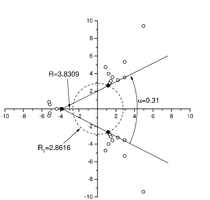
By performing diagonal Padé approximants on this series, we obtain, the distribution of singularities as shown in fig. 4. From this we observe that:
- 1.
the largest possible value of the parameter of the mapping method does not coincide with the radius of convergence of the Maclaurin series (noted in fig. 4). But, this time the radius of convergence cannot be chosen as reference to determine the optimal value of as it would follow from the idealized scheme of fig. 1 of [24], this is because:
- 2.
farther singularities in the half plane would prevent the convergence of the mapping method, so that
- 3.
the effective maximal optimal value of () is small and can be significantly enlarged only if is considerably diminished.
As consequence of this unfavorable singularity distribution, the mapping method for the optimal values and , converges only very slowly (see fig. 5) and, with , we have obtained the poor estimate Smaller values of yield slightly improved convergences which remain slow however. Nevertheless the convergence (even slow) of the method indicates that the distribution of singularities of fig. 4 is correct. Despite this fact, Padé approximants do not yield any estimate of .

4 Summary and conclusion
We have presented, compared and discussed the efficiency of three quasi-analytic methods for solving a BVP: the Taylor series, the Padé and the conformal mapping methods. After having reminded that the first method almost always requires the recourse to analytical continuation procedures to be efficient, our interest has been focused on the latter two.
We have emphasized that the Padé-Hankel method is indeed the “minimal” version of the standard Padé method and explained why it is not always efficient. In particular we have shown that its efficiency is closely related with the possibility of pushing to infinity a movable singularity. The conformal mapping always works but (obviously by construction) its efficiency depends on the analytic properties of the solutions sought.
With a view to present a fairly comprehensive discussion, we have successively considered six different configurations of ODE and initial conditions which yield more and more constraining analytic properties. We have shown that Padé approximants may be used to determine correctly the singularities distribution which allows an efficient determination of the values of the two parameters and of the conformal mapping method [see eq. (15)]. In each case of ODE considered we have empirically discussed the conditions of uniqueness of the solution defined in , this unique solution appears as the envelope of a family of solutions having moving singularities, when such a family of solutions does not exist then an infinite number of solutions are defined in and “minimal” procedures (like the Padé-Hankel method) do not work.
Contrary to the mapping method, the Padé-Hankel method (when it works) is comparatively more and more efficient as the analytic properties harden but it is limited by its awkwardness. The mapping method is more sophisticated and smoother. Provided the analytic properties of the solutions are favorable, it is useful when a high accuracy is required.
Acknowledgments We thank B. Boisseau and H. Giacomini for their useful remarks and comments relative to this work. We are also indebted to the referees for their useful suggestions.
Appendix A Expansions of solutions about particular points
Asymptotic expansions such as (28, 35, etc…) and expansions about a movable singularity such as (27, 36, etc…) may be determined following a similar procedure. The main difference with the expression of the generic solution as a Taylor series is that the terms are not necessarily integer powers of the independent variables. For example, it may involve also powers of logarithms. Sometimes the leading term is not a power but an exponential or a logarithm. This prevents us from using a general systematic algorithm to get the terms of such expansions.
As an illustration we present below the example of the asymptotic expansion of the solution of the Polchinski fixed point equation. The obtention of the local expansion about a movable singularity is very similar and will not be made explicit here.
A.1 Asymptotic expansion of the solution of the Polchinski equation
Let us consider the ODE (24). We want to show that it admits the one-parameter solution (28) as . Although not obliged, it is convenient to perform the following change:
| (86) |
then (24) reads:
| (87) |
Assuming that is small, we try to find a local solution to this ODE under the following form:
| (88) |
where and are the unknowns. It is easy to see that (88) generates three different powers of in the ODE: , and . To get a solution (locally valid) one must first determine the leading power for small and second impose that its coefficient vanishes. These two conditions should determine the values of and .
Since is small, the smallest power prevails, then we distinguish three possibilities:
- 1.
, the leading power is , but the vanishing of the global coefficient imposes (whatever ) what is incompatible with the hypothesis.
- 2.
, the power prevails, but the vanishing of the global coefficient imposes (whatever ) what is incompatible with the hypothesis.
- 3.
, the two powers and are equal and the vanishing of the global coefficient occurs for or .
The leading term of the asymptotic expansion is thus 1. To get the next term we try the following form:
| (89) |
in which the second term is smaller than the first one, i.e. , for consistency. Introduced into the ODE, this expansion about gives the same set of powers of as previously. The leading power is thus . The vanishing of the global coefficient implies that whatever . That is an acceptable solution.
The arbitrariness of the amplitude provides the first arbitrary constant that is noted in (28).
The local expansion of the solution about may be continued by considering the next correction:
and so on and so forth.
In the present case, is the only arbitrary constant appearing in the asymptotic expansion. It is important to know the maximal number of arbitrary parameters in the solution (sometimes called “resonances” in the expansion about a movable point). However, it may occur that the arbitrary constants appear lately in the expansion [e.g. see (36)] which, in addition, may be very complicated. There is a convenient way to quickly know the values of that are associated to the arbitrary constants in the expansion without having to calculate it explicitly. Once the leading term of the expansion is known, one considers the generic correction as in (89) then it suffices to look at the vanishing of the linear-in- contribution to the ODE. The resulting constraint provides an equation for . In the present example there is a unique acceptable solution to this equation: , there is thus only one arbitrary constant ().
References
- [1] H. Blasius, Grenzschichten in Fhissigkeiten mit kleiner Reibung, in Translation: The boundary layers in fluids with little friction, NACA TM (1950) 1256, Z. Math. Phys. Vol. 56 (1908) 1.
- [2] H. Weyl, Concerning the Differential Equations of Some Boundary Layer Problems, Proc. Nat. Acad. Sci. 27 (1941) 578.
- [3] C. Bervillier, B. Boisseau and H. Giacomini, Analytical approximation schemes for solving exact renormalization group equations in the local potential approximation, Nucl. Phys. B 789 (2008) 525. [arXiv:0706.0990v1]
- [4] F. M. Fernández, Direct calculation of accurate Siegert eigenvalues, J. Phys. A 28 (1995) 4043.
- [5] F. M. Fernández, Q. Ma and R. H. Tipping, Eigenvalues of the Schrödinger equation via the Riccati-Padé method, Phys. Rev. A 40 (1989) 6149.
- [6] F. M. Fernández, G. I. Frydman and E. A. Castro, Tight bounds to the Schrödinger equation eigenvalues, J. Phys. A 22 (1989) 641.
- [7] B. Boisseau, P. Forgács and H. Giacomini, An analytical approximation scheme to two point boundary value problems of ordinary differential equations, J. Phys. A 40 (2007) F215. [arXiv:hep-th/0611306]
- [8] D. Leonard and P. Mansfield, A modified Borel summation technique, unpublished (2007). [arXiv:0708.2201]
- [9] D. Leonard and P. Mansfield, Solving the anharmonic oscillator: tuning the boundary condition , J. Phys. A 40 (2007) 10291. [arXiv:quant-ph/0703262]
- [10] C. Bervillier, Conformal mappings versus other Taylor series methods for solving ordinary differential equations: illustration on anharmonic oscillators., J. Phys. A 42 (2009) 485202. [arXiv:0812.2262]
- [11] P. Amore and F. M. Fernández, Rational approximation for two-point boundary value problems, unpublished (2007). [arXiv:0705.3862]
- [12] M. van Dyke, in Perturbation methods in fluid mechanics, Acad. Press, 1964.
- [13] J. P. Boyd, The Blasius function in the complex plane, Experiment. Math. 8 (1999) 381.
- [14] J. P. Boyd, Padé approximant algorithm for solving nonlinear ODE boundary value problems on an unbounded domain, Comput. Phys. 11 (1997) 299.
- [15] J. Polchinski, Renormalization and effective lagrangians, Nucl. Phys. B 231 (1984) 269.
- [16] C. Bagnuls and C. Bervillier, Exact renormalization group equations. An introductory review. , Phys. Rep. 348 (2001) 91. [arXiv:hep-th/0002034] B. Delamotte, An Introduction to the Nonperturbative Renormalization Group, in Order, Disorder and Criticality. Advanced Problems of Phase Transition Theory, Vol 2, p. 1, Ed. by Yu. Holovatch, World Scientific, Publ. Co., Singapore, 2007. [arXiv:cond-mat/0702365] O. J. Rosten, Fundamentals of the exact renormalization group, unpublished (2010). [arXiv:1003.1366]
- [17] L. H. Thomas, The calculation of atomic fields, Proc. Cambridge Phil. Soc. 23 (1927) 542.
- [18] E. Fermi, Un Metodo Statistico per la Determinazione di alcune Prioprietà dell’Atomo, Rend. Accad. Naz. Lincei 6 (1927) 602.
- [19] T. Hayat, F. Shahzad and M. Ayub, Analytical solution for the steady flow of the third grade fluid in a porous half space, Appl. Math. Modell. 31 (2007) 2424.
- [20] F. Ahmad, A simple analytical solution for the steady flow of a third grade fluid in a porous half space, Comm. Nonlinear Sci. Numer. Simul. 14 (2009) 2848.
- [21]
http://en.wikipedia.org/wiki/Power_series_solution_of_differential_equations
(2 may 2011) - [22] A. Margaritis, G. Ódor and A. Patkós, Series expansion solution of the Wegner-Houghton renormalisation group equation, Z. Phys. C 39 (1988) 109.
- [23] G. A. Baker, Jr, in Essentials of Padé Approximants, Acad. Press, 1975. G. A. Baker, Jr and P. Graves-Morris, in Pade Approximants, Part I, Basic Theory, Encyclopedia of Mathematics Vol. 13, Addison Wesley, 1981; ibid., Part II, Extensions and Applications, Encyclopedia of Mathematics Vol. 14, Addison Wesley, 1996.
- [24] C. Bervillier, B. Boisseau and H. Giacomini, Analytical approximation schemes for solving exact renormalization group equations. II Conformal mappings, Nucl. Phys. B 801 (2008) 296. [arXiv:0802.1970]
- [25] C. M. Andersen and J. F. Geer, Power Series expansions for the frequency and period of the limit cycle of the Van Der Pol equation, SIAM J. Appl. Math. 42 (1982) 678.
- [26] R. Conte and M. Musette, in The Painleve Handbook, Springer, 2008.
- [27] R. Conte, The Painlevé approach to nonlinear ordinary differential equations, unpublished (1997). [arXiv:solv-int/9710020]
- [28] A. Mambriani, Su un teorema relativo alle equazioni differenziali ordinarie del 2∘ ordine, unpublished (1929).
- [29] E. Hille, “On the Thomas-Fermi equation”, Proc. Nat. Acad. Sci. 62 (1969) 7.
- [30] A. Sommerfeld, Asymptotische integration der differentialgleichung des Thomas-Fermischen atoms, Z. Phys. A 78 (1932) 283.
- [31] F. M. Fernández, Rational approximation to the Thomas-Fermi equation, Appl. Math. Comp. 217 (2011). [arXiv:0803.2163]
- [32] F. M. Fernández, Comment on: ”Series solution to the Thomas-Fermi equation” [Phys. Lett. A 365 (2007) 111], Phys. Lett. A 372 (2008) 5258.
- [33] S. Abbasbandy and T. Hayat, Solution of the MHD Falkner-Skan flow by Hankel-Padé method, Phys. Lett. A 373 (2009) 731.
- [34] Z. Belhachmi, B. Brighi and K. Taous, On the concave solutions of the Blasius equation, Acta Math. Univ. Comenianae LXIX (2000) 199.
- [35] J. P. Boyd, The Blasius function: computations before computers, the value of tricks, undergraduate projects, and open research problems, SIAM Review 50 (2008) 791.
- [36] C. Töpfer, Bemerkungen zu dem Aufsatz yon H. Blasius, ”Grenzschichten in Fliissigkeiten mit kleiner Reibung”., Z. Math. Phys. 60 (1912) 397.
- [37] R. Fazio, The Blasius problem formulated as a free boundary value problem, Acta Mech. 95 (1992) 1.
- [38] A. Asaithambi, Solution of the Falkner-Skan equation by recursive evaluation of Taylor coefficients, J. Comp. Appl. Math. 176 (2005) 203.
- [39] J. Y. Parlange, R. D. Braddock and G. Sander, Analytical approximations to the solution of the Blasius equation, Acta Mech. 38 (1981) 119.
- [40] L.-T. Yu and C.-K. Chen, The solution of the Blasius equation by the differential transformation method, Mathl. Comput. Modelling 28 (1998) 101.
- [41] S.-J. Liao, A uniformly valid analytic solution of two-dimensional viscous flow over a semi-infinite flat plate, J. Fluid Mech. 385 (1999) 101.
- [42] L. Howarth, On the solution of the laminar boundary layer equations, Proc. R. Soc. Lond. A 164 (1938) 547.
- [43] F. M. Allan, Similarity solutions of a boundary layer problem over moving surfaces, Appl. Math. Lett. 10 (1997) 81.
- [44] S.-J. Liao, in Beyond Perturbation: Introduction to the Homotopy Analysis Method, Chapman and Hall / CRC, 2003.