Synthesizing Robust Plans under Incomplete Domain Models
Abstract
Most current planners assume complete domain models and focus on generating correct plans. Unfortunately, domain modeling is a laborious and error-prone task. While domain experts cannot guarantee completeness, often they are able to circumscribe the incompleteness of the model by providing annotations as to which parts of the domain model may be incomplete. In such cases, the goal should be to generate plans that are robust with respect to any known incompleteness of the domain. In this paper, we first introduce annotations expressing the knowledge of the domain incompleteness, and formalize the notion of plan robustness with respect to an incomplete domain model. We then propose an approach to compiling the problem of finding robust plans to the conformant probabilistic planning problem. We present experimental results with Probabilistic-FF, a state-of-the-art planner, showing the promise of our approach.
1. Introduction
In the past several years, significant strides have been made in scaling up plan synthesis techniques. We now have technology to routinely generate plans with hundreds of actions. All this work, however, makes a crucial assumption–that a complete model of the domain is specified in advance. While there are domains where knowledge-engineering such detailed models is necessary and feasible (e.g., mission planning domains in NASA and factory-floor planning), it is increasingly recognized (c.f. [2010, 2007]) that there are also many scenarios where insistence on correct and complete models renders the current planning technology unusable. What we need to handle such cases is a planning technology that can get by with partially specified domain models, and yet generate plans that are “robust” in the sense that they are likely to execute successfully in the real world.
This paper addresses the problem of formalizing the notion of plan robustness with respect to an incomplete domain model, and connects the problem of generating a robust plan under such model to conformant probabilistic planning [1995, 2003, 2006, 2007]. Following Garland & Lesh (?), we shall assume that although the domain modelers cannot provide complete models, often they are able to provide annotations on the partial model circumscribing the places where it is incomplete. In our framework, these annotations consist of allowing actions to have possible preconditions and effects (in addition to the standard necessary preconditions and effects).
As an example, consider a variation of the Gripper domain, a well-known planning benchmark domain. The robot has one gripper that can be used to pick up balls, which are of two types light and heavy, from one room and move them to another room. The modeler suspects that the gripper may have an internal problem, but this cannot be confirmed until the robot actually executes the plan. If it actually has the problem, the execution of the pick-up action succeeds only with balls that are not heavy, but if it has no problem, it can always pickup all types of balls. The modeler can express this partial knowledge about the domain by annotating the action with a statement representing the possible precondition that balls should be light.
Incomplete domain models with such possible preconditions/effects implicitly define an exponential set of complete domain models, with the semantics that the real domain model is guaranteed to be one of these. The robustness of a plan can now be formalized in terms of the cumulative probability mass of the complete domain models under which it succeeds. We propose an approach that compiles the problem of finding robust plans into the conformant probabilistic planning problem. We present experimental results showing scenarios where the approach works well, and also discuss aspects of the compilation that cause scalability issues.
2. Related Work
Although there has been some work on reducing the “faults” in plan execution (e.g. the work on k-fault plans for non-deterministic planning [2004]), it is based in the context of stochastic/non-deterministic actions rather than incompletely specified ones. The semantics of the possible preconditions/effects in our incomplete domain models differ fundamentally from non-deterministic and stochastic effects. Executing different instances of the same pick-up action in the Gripper example above would either all fail or all succeed, since there is no uncertainty but the information is unknown at the time the model is built. In contrast, if the pick-up action’s effects are stochastic, then trying the same picking action multiple times increases the chances of success.
Garland & Lesh (?) share the same objective with us on generating robust plans under incomplete domain models. However, their notion of robustness, which is defined in terms of four different types of risks, only has tenuous heuristic connections with the likelihood of successful execution of plans. Robertson & Bryce (?) focuses on the plan generation in Garland & Lesh model, but their approach still relies on the same unsatisfactory formulation of robustness. The work by Fox et al (?) also explores robustness of plans, but their focus is on temporal plans under unforeseen execution-time variations rather than on incompletely specified domains. Our work can also be categorized as one particular instance of the general model-lite planning problem, as defined in [2007], in which the author points out a large class of applications where handling incomplete models is unavoidable due to the difficulty in getting a complete model.
3. Problem Formulation
We define an incomplete domain model as , where is a set of propositions, is a set of actions that might be incompletely specified. We denote and as the true and false truth values of propositions. A state is a set of propositions. In addition to proposition sets that are known as its preconditions , add effects and delete effects , each action also contains:
- •
Possible precondition set contains propositions that action might need as its preconditions.
- •
Possible add (delete) effect set () contains propositions that the action might add (delete, respectively) after its execution.
In addition, each possible precondition, add and delete effect of the action is associated with a weight , and () representing the domain modeler’s assessment of the likelihood that will actually be realized as a precondition, add and delete effect of (respectively) during plan execution. Possible preconditions and effects whose likelihood of realization is not given are assumed to have weights of .
Given an incomplete domain model , we define its completion set as the set of complete domain models whose actions have all the necessary preconditions, adds and deletes, and a subset of the possible preconditions, possible adds and possible deletes. Since any subset of , and can be realized as preconditions and effects of action , there are exponentially large number of possible complete domain models , where . For each complete model , we denote the corresponding sets of realized preconditions and effects for each action as , and ; equivalently, its complete sets of preconditions and effects are , and .
The projection of a sequence of actions from an initial state according to an incomplete domain model is defined in terms of the projections of from according to each complete domain model :
| (1) |
where the projection over complete models is defined in the usual STRIPS way, with one important difference. The result of applying an action in a state where the preconditions of are not satisfied is taken to be (rather than as an undefined state).11 1 We shall see that this change is necessary so that we can talk about increasing the robustness of a plan by adding additional actions.
A planning problem with incomplete domain is where is the set of propositions that are true in the initial state, and is the set of goal propositions. An action sequence is considered a valid plan for if solves the problem in at least one completion of . Specifically, .
Modeling Issues in Annotating Incompleteness: From the modeling point of view, the possible precondition and effect sets can be modeled at either the grounded action or action schema level (and thus applicable to all grounded actions sharing the same action schema). From a practical point of view, however, incompleteness annotations at ground level hugely increase the burden on the domain modeler. To offer a flexible way in modeling the domain incompleteness, we allow annotations that are restricted to either specific variables or value assignment to variables of an action schema. In particular:
- •
Restriction on value assignment to variables: Given variables with domains , one can indicate that is a possible precondition/effect of an action schema when some variables have values (). Those possible preconditions/effects can be specified with the annotation for the action schema . More generally, we allow the domain writer to express a constraint on the variables in the construct. The annotation means that is a possible precondition/effect of an instantiated action () if and only if the assignment satisfies the constraint . This syntax subsumes both the annotations at the ground level when , and at the schema level if (or the construct is not specified).
- •
Restriction on variables: Instead of constraints on explicit values of variables, we also allow the possible preconditions/effects of an action schema to be dependent on some specific variables without any knowledge of their restricted values. This annotation essentially requires less amount of knowledge of the domain incompleteness from the domain writer. Semantically, the possible precondition/effect of an action schema means that (1) there is at least one instantiated action () having as its precondition, and (2) for any two assignments such that (), either both and are preconditions of the corresponding actions, or they are not. Similar to the above, the construct also subsumes the annotations at the ground level when , and at the schema level if (or the field is not specified).
Another interesting modeling issue is the correlation among the possible preconditions and effects across actions. In particular, the domain writer might want to say that two actions (or action schemas) will have specific possible preconditions and effects in tandem. For example, we might say that the second action will have a particular possible precondition whenever the first one has a particular possible effect. We note that annotations at the lifted level introduce correlations among possible preconditions and effects at the ground level.
Although our notion of plan robustness and approach to generating robust plans (see below) can be adapted to allow such flexible annotations and correlated incompleteness, for ease of exposition we limit our discussion to uncorrelated possible precondition and effect annotations specified at the schema level (i.e. without using the and constructs).
4. A Robustness Measure for Plans
Given an incomplete domain planning problem , a valid plan (by our definition above) need only to succeed in at least one completion of . Given that can be exponentially large in terms of possible preconditions and effects, validity is too weak to guarantee on the quality of the plan. What we need is a notion that succeeds in most of the highly likely completions of . We do this in terms of a robustness measure.
The robustness of a plan for the problem is defined as the cumulative probability mass of the completions of under which succeeds (in achieving the goals). More formally, let be the probability distribution representing the modeler’s estimate of the probability that a given model in is the real model of the world (such that ). The robustness of is defined as follows:
| (2) |
It is easy to see that if , then is a valid plan for .
Note that given the uncorrelated incompleteness assumption, the probability for a model can be computed as the product of the weights , , and for all and its possible preconditions/effects if is realized in the model (or the product of their “complement” , , and if is not realized).

Example: Figure 1 shows an example with an incomplete domain model with and and a solution plan for the problem . The incomplete model is: , , , , , ; , , , , , . Given that the total number of possible preconditions and effects is 3, the total number of completions () is , for each of which the plan may succeed or fail to achieve , as shown in the table. The robustness value of the plan is if is the uniform distribution. However, if the domain writer thinks that is very likely to be a precondition of and provides , the robustness of decreases to (as intutively, the last four models with which succeeds are very unlikely to be the real one). Note that under the STRIPS model where action failure causes plan failure, the plan would considered failing to achieve in the first two complete models, since is prevented from execution.
4.1 A Spectrum of Robust Planning Problems
Given this set up, we can now talk about a spectrum of problems related to planning under incomplete domain models:
- Robustness Assessment (RA):
-
Given a plan for the problem , assess the robustness of .
- Maximally Robust Plan Generation (RG∗):
-
Given a problem , generate the maximally robust plan .
- Generating Plan with Desired Level of Robustness (RGρ):
-
Given a problem and a robustness threshold (), generate a plan with robustness greater than or equal to .
- Cost-sensitive Robust Plan Generation (RG):
-
Given a problem and a cost bound , generate a plan of maximal robustness subject to cost bound (where the cost of a plan is defined as the cumulative costs of the actions in ).
- Incremental Robustification (RIc):
-
Given a plan for the problem , improve the robustness of , subject to a cost budget .
The problem of assessing robustness of plans, RA, can be tackled by compiling it into a weighted model-counting problem. For plan synthesis problems, we can talk about either generating a maximally robust plan, RG∗, or finding a plan with a robustness value above the given threshold, RGρ. A related issue is that of the interaction between plan cost and robustness. Often, increasing robustness involves using additional (or costlier) actions to support the desired goals, and thus comes at the expense of increased plan cost. We can also talk about cost-constrained robust plan generation problem RG. Finally, in practice, we are often interested in increasing the robustness of a given plan (either during iterative search, or during mixed-initiative planning). We thus also have the incremental variant RIc.
In this paper, we will focus on RGρ, the problem of synthesizing plan with at least a robustness value of .
5. Compilation to Conformant Probabilistic Planning
In this section, we will show that the problem of generating plan with at least robustness, RGρ, can be compiled into an equivalent conformant probabilistic planning problem. The most robust plan can then be found with a sequence of increasing threshold values.
5.1 Conformant Probabilistic Planning
Following the formalism in [2007], a domain in conformant probabilistic planning (CPP) is a tuple , where and are the sets of propositions and probabilistic actions, respectively. A belief state is a distribution of states (we denote if ). Each action is specified by a set of preconditions and conditional effects . For each , is the condition set and determines the set of outcomes that will add and delete proposition sets , into and from the resulting state with the probability ( , ). All condition sets of the effects in are assumed to be mutually exclusive and exhaustive. The action is applicable in a belief state if for all , and the probability of a state in the resulting belief state is , where is the conditional effect such that , and is the set of outcomes such that .
Given the domain , a problem is a quadruple , where is an initial belief state, is a set of goal propositions and is the acceptable goal satisfaction probability. A sequence of actions is a solution plan for if is applicable in the belief state (assuming ), which results in (), and it achieves all goal propositions with at least probability.
5.2 Compilation
Given an incomplete domain model and a planning problem , we now describe a compilation that translates the problem of synthesizing a solution plan for such that to a CPP problem . At a high level, the realization of possible preconditions and effects , of an action can be understood as being determined by the truth values of hidden propositions , and that are certain (i.e. unchanged in any world state) but unknown. Specifically, the applicability of the action in a state depends on possible preconditions that are realized (i.e. ), and their truth values in . Similarly, the values of and are affected by in the resulting state only if they are realized as add and delete effects of the action (i.e., , ). There are totally realizations of the action , and all of them should be considered simultaneously in checking the applicability of the action and in defining corresponding resulting states.
With those observations, we use multiple conditional effects to compile away incomplete knowledge on preconditions and effects of the action . Each conditional effect corresponds to one realization of the action, and can be fired only if whenever , and adding (removing) an effect () into (from) the resulting state depending on the values of (, respectively) in the realization.
While the partial knowledge can be removed, the hidden propositions introduce uncertainty into the initial state, and therefore making it a belief state. Since the action may be applicable in some but rarely all states of a belief state, certain preconditions should be modeled as conditions of all conditional effects. We are now ready to formally specify the resulting domain and problem .
For each action , we introduce new propositions , , and their negations , , for each , and to determine whether they are realized as preconditions and effects of in the real domain.22 2 These propositions are introduced once, and re-used for all actions sharing the same schema with . Let be the set of those new propositions, then is the proposition set of .
Each action is made from one action such that , and consists of conditional effects . For each conditional effect :
- •
is the union of the following sets:
- –
the certain preconditions ,
- –
the set of possible preconditions of that are realized, and hidden propositions representing their realization: ,
- –
the set of hidden propositions corresponding to the realization of possible add (delete) effects of : (, respectively);
- –
- •
the single outcome of is defined as , , and ,
where , and represent the sets of realized preconditions and effects of the action. In other words, we create a conditional effect for each subset of the union of the possible precondition and effect sets of the action . Note that the inclusion of new propositions derived from , , and their “complement” sets , , makes all condition sets of the action mutually exclusive. As for other cases (including those in which some precondition in is excluded), the action has no effect on the resulting state, they can be ignored. The condition sets, therefore, are also exhaustive.
The initial belief state consists of states such that iff (), each represents a complete domain model and with the probability . The goal is , and the acceptable goal satisfaction probability is .
Theorem 1.
Given a plan for the problem , and where is the compiled version of () in . Then iff achieves all goals with at least probability in .
Proof (sketch).
According to the compilation, there is one-to-one mapping between each complete model in and a (complete) state in . Moreover, if has a probability of to be the real model, then also has a probability of in the belief state of .
Given our projection over complete model , executing from the state with respect to results in a sequence of complete state . On the other hand, executing from in results in a sequence of belief states . With the note that iff (), by induction it can be shown that iff (). Therefore, iff .
Since all actions are deterministic and has a probability of in the belief state of , the probability that achieves is , which is equal to as defined in Equation 2. This proves the theorem. ∎
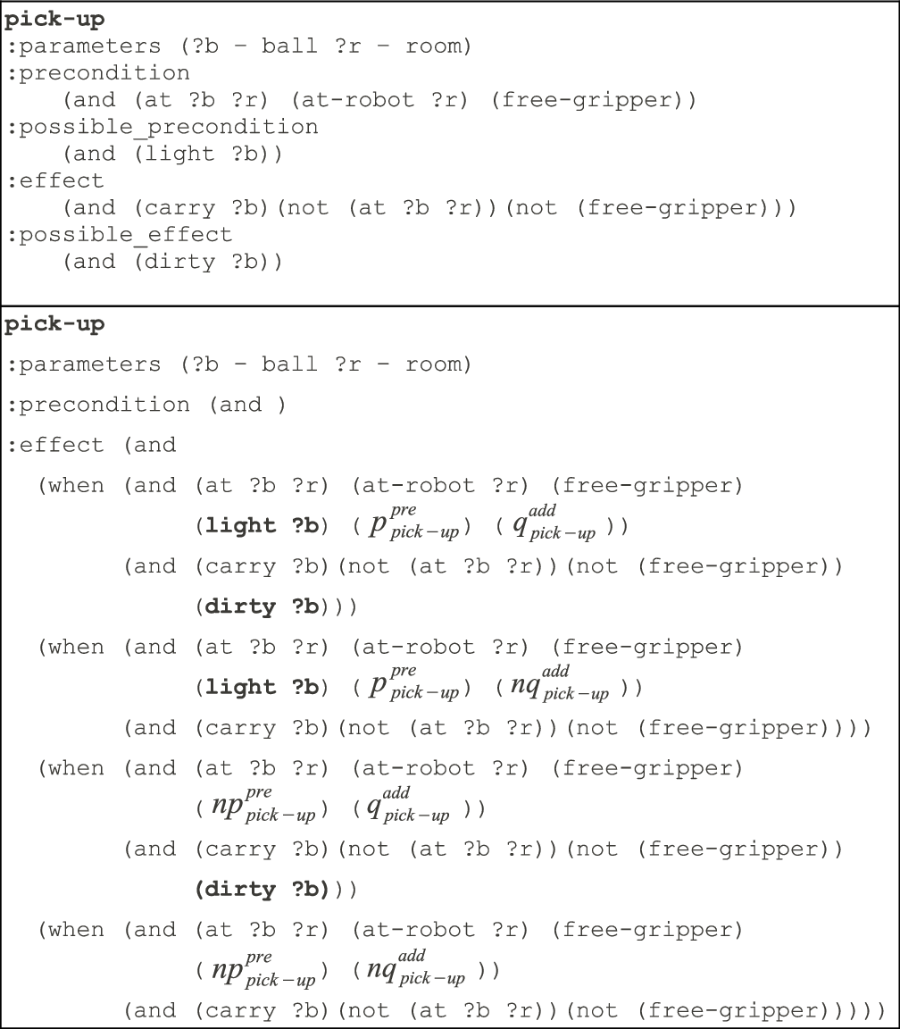
Example: Consider the action pick-up(?b - ball,?r - room) in the Gripper domain as described above. In addition to the possible precondition (light ?b) on the weight of the ball ?b, we also assume that since the modeler is unsure if the gripper has been cleaned or not, she models it with a possible add effect (dirty ?b) indicating that the action might make the ball dirty. Figure 2 shows both the original and the compiled specification of the action.
6. Experimental Results
We tested the compilation with Probabilistic-FF (PFF), a state-of-the-art planner, on a range of domains in the International Planning Competition.We first discuss the results on the variants of the Logistics and Satellite domains, where domain incompleteness is deliberately modeled on the preconditions and effects of actions (respectively). Our purpose here is to observe how generated plans are robustified to satisfy a given robustness threshold, and how the amount of incompleteness in the domains affects the plan generation phase. We then describe the second experimental setting in which we randomly introduce incompleteness into IPC domains, and discuss the feasibility of our approach in this setting.33 3 The experiments were conducted using an Intel Core2 Duo 3.16GHz machine with 4Gb of RAM, and the time limit is 15 minutes.
Domains with deliberate incompleteness
Logistics: In this domain, each of the two cities and has an airport and a downtown area. The transportation between the two distant cities can only be done by two airplanes and . In the downtown area of (), there are three heavy containers that can be moved to the airport by a truck . Loading those containers onto the truck in the city , however, requires moving a team of robots (), initially located in the airport, to the downtown area. The source of incompleteness in this domain comes from the assumption that each pair of robots and () are made by the same manufacturer , both therefore might fail to load a heavy container.44 4 The uncorrelated incompleteness assumption applies for possible preconditions of action schemas specified for different manufacturers. It should not be confused here that robots and of the same manufacturer can independently have fault. The actions loading containers onto trucks using robots made by a particular manufacturer (e.g., the action schema load-truck-with-robots-of-M1 using robots of manufacturer ), therefore, have a possible precondition requiring that containers should not be heavy. To simplify discussion (see below), we assume that robots of different manufacturers may fail to load heavy containers, though independently, with the same probability of . The goal is to transport all three containers in the city to , and vice versa. For this domain, a plan to ship a container to another city involves a step of loading it onto the truck, which can be done by a robot (after moving it from the airport to the downtown). Plans can be made more robust by using additional robots of different manufacturer after moving them into the downtown areas, with the cost of increasing plan length.
Satellite: In this domain, there are two satellites and orbiting the planet Earth, on each of which there are instruments (, ) used to take images of interested modes at some direction in the space. For each , the lenses of instruments ’s were made from a type of material , which might have an error affecting the quality of images that they take. If the material actually has error, all instruments ’s produce mangled images. The knowledge of this incompleteness is modeled as a possible add effect of the action taking images using instruments made from (for instance, the action schema take-image-with-instruments-M1 using instruments of type ) with a probability of , asserting that images taken might be in a bad condition. A typical plan to take an image using an instrument, e.g. of type on the satellite , is first to switch on , turning the satellite to a ground direction from which can be calibrated, and then taking image. Plans can be made more robust by using additional instruments, which might be on a different satellite, but should be of different type of materials and can also take an image of the interested mode at the same direction.
| – | |||||
| – | |||||
Table 1 and 2 shows respectively the results in the Logistics and Satellite domains with and . The number of complete domain models in the two domains is . For Satellite domain, the probabilities ’s range from , ,… to when increases from , , … to . For each specific value of and , we report where is the length of plan and is the running time (in seconds). Cases in which no plan is found within the time limit are denoted by “–”, and those where it is provable that no plan with the desired robustness exists are denoted by “”.
Observations on fixed value of : In both domains, for a fixed value of we observe that the solution plans tend to be longer with higher robustness threshold , and the time to synthesize plans is also larger. For instance, in Logistics with , the plan returned has actions if , whereas -length plan is needed if increases to . Since loading containers using the same robot multiple times does not increase the chance of success, more robots of different manufacturers need to move into the downtown area for loading containers, which causes an increase in plan length. In the Satellite domain with , similarly, the returned plan has actions when , but requires actions if —more actions need to calibrate an instrument of different material types in order to increase the chance of having a good image of interested mode at the same direction.
Since the cost of actions is currently ignored in the compilation approach, we also observe that more than the needed number of actions have been used in many solution plans. In the Logistics domain, specifically, it is easy to see that the probability of successfully loading a container onto a truck using robots of () different manufacturers is . As an example, however, robots of all five manufacturers are used in a plan when , whereas using those of three manufacturers is enough.
Observations on fixed value of : In both domains, we observe that the maximal robustness value of plans that can be returned increases with higher number of manufacturers (though the higher the value of is, the higher number of complete models is). For instance, when there is not any plan returned with at least in the Logistics domain, and with in the Satellite domain. Intuitively, more robots of different manufacturers offer higher probability of successfully loading a container in the Logistics domain (and similarly for instruments of different materials in the Satellite domain).
Finally, it may take longer time to synthesize plans with the same length when is higher—in other words, the increasing amount of incompleteness of the domain makes the plan generation phase harder. As an example, in the Satellite domain, with it takes seconds to synthesize a -length plan when there are possible add effects at the schema level of the domain, whereas the search time is only seconds when . With , no plan is found within the time limit when , although a plan with robustness of exists in the solution space. It is the increase of the branching factors and the time spent on satisfiability test and weighted model-counting used inside the planner that affect the search efficiency.
Domains with random incompleteness
We built a program to generate an incomplete domain model from a deterministic one by introducing new propositions into each domain (all are initially ). Some of those new propositions were randomly added into the sets of possible preconditions/effects of actions. Some of them were also randomly made certain add/delete effects of actions. With this strategy, each solution plan in an original deterministic domain is also a valid plan, as defined earlier, in the corresponding incomplete domain. Our experiments with the Depots, Driverlog, Satellite and ZenoTravel domains indicate that because the annotations are random, there are often fewer opportunities for the PFF planner to increase the robustness of a plan prefix during the search. This makes it hard to generate plans with a desired level of robustness under given time constraint.
In summary, our experiments on the two settings above suggest that the compilation approach based on the PFF planner would be a reasonable method for generating robust plans in domains and problems where there are chances for robustifying existing action sequences in the search space.
7. Conclusion and Future Work
In this paper, we motivated the need for synthesizing robust plans under incomplete domain models. We introduced annotations for expressing domain incompleteness, formalized the notion of plan robustness, and showed an approach to compile the problem of generating robust plans into conformant probabilistic planning. We presented empirical results showing the promise of our approach. For future work, we are developing a planning approach that directly takes the incompleteness annotations into account during the search, and compare it with our current compilation method. We also plan to consider the problem of robustifying a given plan subject to a provided cost bound.
Acknowledgement: This research is supported in part by ONR grants N00014-09-1-0017 and N00014-07-1-1049, the NSF grant IIS-0905672, and by DARPA and the U.S. Army Research Laboratory under contract W911NF-11-C-0037. The content of the information does not necessarily reflect the position or the policy of the Government, and no official endorsement should be inferred. We thank William Cushing for several helpful discussions.
References
- [2006] Bryce, D.; Kambhampati, S.; and Smith, D. 2006. Sequential monte carlo in probabilistic planning reachability heuristics. Proceedings of ICAPS’06.
- [2007] Domshlak, C., and Hoffmann, J. 2007. Probabilistic planning via heuristic forward search and weighted model counting. JAIR 30(1):565–620.
- [2006] Fox, M.; Howey, R.; and Long, D. 2006. Exploration of the robustness of plans. In AAAI.
- [2002] Garland, A., and Lesh, N. 2002. Plan evaluation with incomplete action descriptions. In AAAI.
- [2010] Hoffmann, J.; Weber, I.; and Kraft, F. 2010. SAP Speaks PDDL. AAAI.
- [2003] Hyafil, N., and Bacchus, F. 2003. Conformant probabilistic planning via CSPs. In Proceedings of the Thirteenth International Conference on Automated Planning and Scheduling, 205–214.
- [2004] Jensen, R.; Veloso, M.; and Bryant, R. 2004. Fault tolerant planning: Toward probabilistic uncertainty models in symbolic non-deterministic planning. In ICAPS.
- [2007] Kambhampati, S. 2007. Model-lite planning for the web age masses: The challenges of planning with incomplete and evolving domain theories. In AAAI.
- [1995] Kushmerick, N.; Hanks, S.; and Weld, D. 1995. An algorithm for probabilistic planning. Artificial Intelligence 76(1-2):239–286.
- [2009] Robertson, J., and Bryce, D. 2009. Reachability heuristics for planning in incomplete domains. In ICAPS’09 Workshop on Heuristics for Domain Independent Planning.