IPMU11-0071
YITP-11-49
Probing AdS Wormholes by Entanglement Entropy
Mitsutoshi Fujita11 1 e-mail: mitsutoshi.fujita@ipmu.jp, Yasuyuki Hatsuda22 2 e-mail: hatsuda@yukawa.kyoto-u.ac.jp and Tadashi Takayanagi33 3 e-mail: tadashi.takayanagi@ipmu.jp
1,3Institute for the Physics and Mathematics of the Universe (IPMU),
University of Tokyo, Kashiwa, Chiba 277-8582, Japan
2Yukawa Institute for Theoretical Physics,
Kyoto University, Kyoto 606-8502, Japan
In this paper, we study the Lorentzian AdS wormhole solutions constructed in arXiv:0808.2481 [hep-th]. Each of them is a classical solution interpolating between an AdS space and a flat space in type IIB supergravity. We calculate the holographic entanglement entropy to probe this geometry. Our analysis shows that there exits a mass gap in its holographic dual gauge theory and that the entanglement between the two boundaries is rather suppressed than that we naively expect for wormholes. We also examine the holographic conductivity on a probe D-brane in this spacetime.
1 Introduction
The AdS/CFT correspondence [2] offers us a powerful way to study quantum gravity on curved spacetimes in a non-perturbative way. In particular, it will be intriguing to understand what the AdS/CFT will predict about quantum gravity on topologically non-trivial spacetimes. In this paper we would like to explore how we can apply the AdS/CFT to asymptotically AdS spacetimes which look like Lorentzian wormholes, called AdS wormholes.
An AdS wormhole spacetime causally connects two different asymptotic regions via a thin tube. Under a suitable energy condition in Einstein gravity, it has been proved that there are no wormhole solutions which connect two disconnected asymptotically AdS boundaries [3]. However, recently wormhole-like solutions have been found in [4, 5, 6] which connect an asymptotically AdS boundary to an asymptotically flat boundary.11 1 There are other classes of AdS wormhole solutions. We can find examples of the Euclidean AdS wormholes [7, 8, 9]. In Lorentzian spacetime, there exists AdS wormholes in the Gauss-Bonnet gravity [10, 11, 12]. Moreover, Lorentzian asymptotic AdS spacetimes with multiple boundaries which are connected via horizons have been studied in [13]. In this paper we will not discuss these. These are smooth solutions in ten or eleven dimensional supergravities. For example, a wormhole solution with a D3-brane charge smoothly interpolates between AdSS5 and . This evades the no-go theorem because the asymptotically AdS boundary appears only one side.
There is a well-known puzzle for an AdS wormhole [7, 8]. Since its boundary consists of two disconnected manifolds, two dual CFTs live on them according to the principle of AdS/CFT. Because the boundaries are disconnected, we expect that the CFTs that live on them are decoupled. However, in the AdS gravity picture, they are connected by a throat and thus there should be non-zero interactions between these two theories. In the black hole geometry, where the two boundaries are connected by an event horizon and these two theories are thermally entangled with each other [14]. In the wormhole case, the interpretation looks puzzling as the temperature of the spacetime is vanishing.
Motivated by these, in this paper, we study the properties of AdS wormhole solutions in order to understand their holographic duals. In particular, we analyze the holographic entanglement entropy [15, 16, 17, 18]. This is because the entanglement entropy [19, 20, 21, 22] is a rather general physical quantity which can be defined in any quantum many body systems and is useful to understand general properties of holography. Refer to [16, 12] for earlier calculations of the entanglement entropy of wormholes in different holographic setups. Moreover, we will also analyze the holographic conductivity as another probe of this spacetime.
This paper is organized as follows: In section two, we give a brief review of the AdS wormhole solutions. In section three we calculate the holographic entanglement entropy. In section four we compute the holographic conductivity by using a probe D-brane. In section five, we summarize conclusions.
2 Brief Review of Lorentzian AdS Wormhole Solutions
One of the most intriguing examples of the AdS wormhole solutions is obtained in type IIB supergravity from a modification of AdSS5 solution [4]
| (1) |
where we defined
| (2) |
Indeed, it is a simple exercise to show that (1) satisfies the equation of motion of type IIB supergravity in ten dimensions (here we set the string coupling to be one just for a simple normalization). The radial coordinate takes values between . We can confirm that (1) is a smooth solution which connects the AdSS5 and the flat space . In the limit , the spacetime approaches the AdSS5 as
| (3) |
where we used and . On the other hand, in the opposite limit , since and , we obtain
| (4) |
where we set . It is obvious that this represents a flat spacetime after an appropriate coordinate transformation. Through this analysis we also learned that the parameter describes the AdS radius, while does the size of the wormhole.
We can dimensionally reduce the this solution (1) to five dimensions [4]. The five dimensional gravity action looks like
| (5) |
where we set .
| (6) | |||
| (7) |
From the metric of this solution, we can show that there are no time-like or null geodesic line which connects the two asymptotic regions [23, 4]. However, there is a non-geodesic time-like trajectory which connects them. This is the reason why the authors of [4] call this an AdS wormhole.
Another important property is the holographic stress energy tensor for the background (1). The only non-trivial component turns out to be
| (8) |
Notice that this breaks the standard energy conditions as the energy is vanishing while the momentum is non-zero. However, this wormhole solution is a smooth solution in type IIB supergravity and can be embedded into string theory. Therefore it is still intriguing to understand the structure of holography for this spacetime. This kind of analysis will help us to understand holography in rather general spacetimes, which is one of the most important problems in string theory.
3 Holographic Entanglement Entropy of AdS5 Wormhole
The entanglement entropy with respect to the subsystem is defined by the von Neumann entropy for the reduced density matrix . The reduced density matrix is defined by tracing out the subsystem , which is the complement of . In quantum field theories, we can specify the subsystem by dividing a time slice into two regions. In this paper we choose the region for is given by a strip whose width is defined by . In order to understand properties of the AdS wormhole solutions, we would like to study the behavior of the entanglement entropy in this section.
In the holographic dual calculation [15, 16], this quantity is given by the area of a codimension two extremal surface as
| (9) |
We require that the boundary of coincides with that of the region and that is homotopic to . If we have several extremal surfaces, then we pick up the one with the smallest area. We will employ the five dimensional metric (6) and analyze its three dimensional minimal surfaces.
Below we consider two cases where the strip extends infinitely (i) in the and and (ii) in the and directions.
3.1 Case 1: Strip extended in the and directions
Let us consider the holographic entanglement entropy for the following subsystem
| (10) |
By the translation symmetry, we can parameterize the surface as
| (11) |
The area functional is given by
| (12) |
where
| (13) |
The equations of motion leads to the following two conserved quantities
| (14) |
where and are integration constants. To define the entanglement entropy at a constant time (e.g. ), we need to require that the subsystem is on the same time slice: . Since we can show that solutions with and do not exist, we focus on the solutions with below. When takes the minimal value , should diverge at this point. This gives the relation between and ,
| (15) |
One can easily solve (14),
| (16) |
The length of the strip is given by . The area is given by
| (17) |
where is the length in the and directions, and we assume . This area is still divergent because the integrand near behaves as
| (18) |
To regularize the area, we put a cut-off at , then the regularized area behaves as . The divergent part is in accord with the standard area law of the entanglement entropy [19]. The cut-off independent finite area is given by
| (19) |

|

|
|
| (a) | (b) | (c) |
The -dependence of length is shown in Fig. 1(a). This figure shows that has a bound at some value of , and the solution exists only for where is the value such that , that is,
| (20) |
Therefore for a small enough value of we have two connected minimal surfaces.
Moreover, for any value of , there are disconnected surfaces given by and , extending from to . At , the surface can end as the area density gets vanishing as follows from the metric (6).
In this way, we have three branches as a function of : two are connected and one is disconnected. In Fig. 1(b), we plot the relation between and the finite part of the area for each surface. Among the three surfaces, we need to select the one with the smallest area. First we can ignore the branch which always takes the largest value. The remaining two branches actually compete with each other: one takes a constant value and the other one has a concave shape. It is important that the constant one intersects with the concave one at some value of (see Fig. 1(b)). This means that for larger than this value , the surface that consists of two disconnected planes () and the plane () has the smaller area than the surface of the solution (16). On the other hand, when we need to choose the concave one. Thus we find a sort of phase transition at .
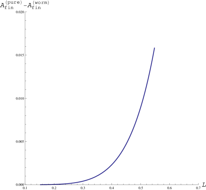
Qualitatively, this behavior looks very similar to the one obtained for gravity duals of confining gauge theories [24, 25, 26], where an analogous phase transition occurs and corresponds to the confinement/deconfinement transition (a similar behavior has recently been confirmed by calculations in lattice gauge theories [27, 28, 29]). This implies that the dual CFT has a mass gap, which will probably correspond to some confining gauge theory. Indeed, we can confirm that the holographic entanglement entropy for the AdS5 wormhole is smaller than that for the pure AdS5 as plotted in Fig. 1(c).
3.2 Case 2: Strip extended in the and direction
Let us next consider the subsystem
| (21) |
If we parameterize the surface as
| (22) |
the action is given by
| (23) |
where
| (24) |
The equations of motion lead to
| (25) |
where and are constants. The solutions are given by
| (26) |
where and
| (27) |
The minimal value is related to and as
| (28) |
As in the previous subsection, we impose the constant time slice condition . This constraint relates the constant to . The area is given by
| (29) |
As well as before, we define the finite part of the area by
| (30) |

|

|
|---|---|
| (a) | (b) |
Once we find from the condition , we can evaluate the length and the area as functions of . We plot the -dependence of and in Fig. 2(a) and (b), respectively, and the relation between and the finite part of the area is shown in Fig. 3 (a). The area again has three branches.

|

|
|
| (a) | (b) | (c) |
As in the previous subsection, the above connected surfaces are defined only for small enough values of and we can find a disconnected surface defined for any . This disconnected surface extends to the range since the area density at is vanishing as mentioned before. Among the connected surfaces constructed in (26) with the constraint ,22 2 The surfaces with have the larger areas than those with , or do not satisfy the null expansion conditions required in [16]. we compute the area of the part as a function of , and find that the area takes a minimal value at (see Fig. 3(b)). Therefore the disconnected surface that has the minimal area is given by the part of the connected one for .
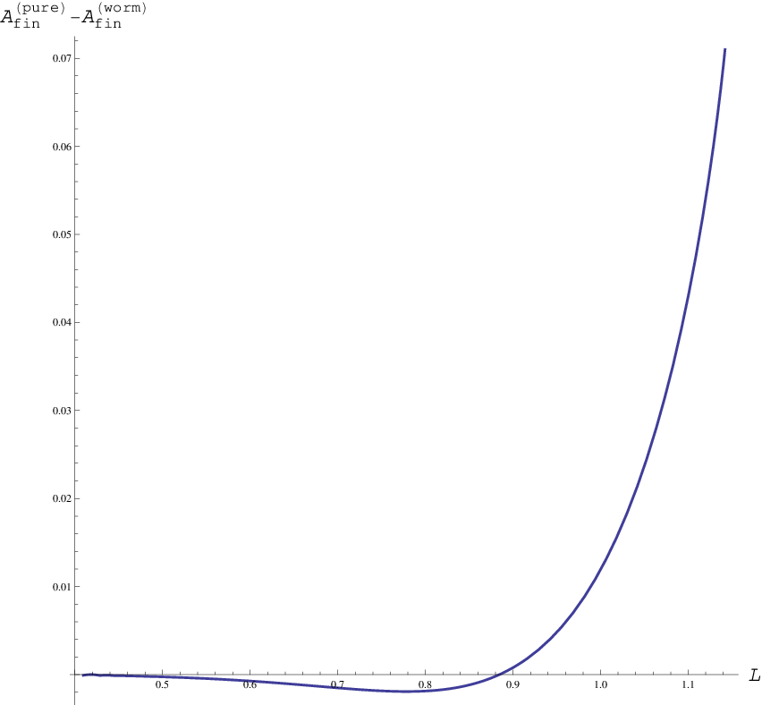
In summary, for this choice of the subsystem, we again encounter a behavior similar to confining gauge theories [24, 25, 26]. For large enough , our entanglement entropy is smaller than that for the pure AdS as shown in Fig.3 (c) and this again suggests that the theory has a mass gap.
One may naturally think that the wormhole geometry suggests that the two holographic duals on the two boundaries are entangled with each other. If this is true, then the entanglement entropy should be greater than that for the pure AdS space. Indeed, as we explain in the appendix A, we can obtain this behavior for an geodesically traversable AdS wormhole (44). The amount of the increased entropy is extensive and therefore the holographic dual looks like a thermal state. However, the metric (44) cannot be embedded into Einstein gravity without violating the null energy condition of matter fields [3].
On the contrary, our holographic results for the AdS wormhole solution (6), which can be realized in type IIB supergravity [4], show that the entropy is reduced as opposed to this naive guess. Also our analysis reveals that the entanglement entropy between the two boundary theories is vanishing. All these tell us that the presence of two boundaries does not cause the quantum entanglement between the two dual theories at least from the viewpoint of the entanglement entropy. It may be possible that this slightly surprising property is generally true in the ‘wormhole’ gravity duals in physically sensible gravity theories. Finally we note that the AdS3 wormhole solutions constructed in [23, 4] also have the same property.
4 Holographic Conductivity
To probe the AdS wormhole, next we would like to study the holographic conductivity. We calculate the AC conductivity on a probe D3-brane in the AdS5 wormhole solution (1). For simplicity, we set . The worldvolume coordinates of the probe D3-brane are given by . The brane is localized in the and direction. The induced metric of the D3-brane then becomes asymptotically in the limit .
Another motivation of this setup is a possibility of constructing a holographic dual of a system with impurities (for earlier works from different viewpoints see [30, 31, 32, 33, 34, 35]). We regard the theory that lives on the asymptotically flat boundary as the one for the impurities sector, while the main quantum system lives on the AdS boundary. Assuming that these impurities only absorb the energy from the outside, we can impose in-going boundary conditions as we will see below. However, notice that we can also impose the Dirichlet boundary condition for which the system looks like a insulator, though we will not discuss this in detail.
4.1 Vanishing Charge Density
We first consider the case where the charge density on the brane is vanishing. In the quadratic order of the worldvolume fields, the Lagrangian is given by the Maxwell theory
| (31) |
where and . Here, the gauge field is normalized properly.
Imposing the gauge fixing , the equations of motion for the vector field become the following differential equation33 3 In this paper, we do not analyze other vector fields and since for , the analysis with finite charge is simpler than that for and . :
| (32) |
In the asymptotically space, the holographic AC conductivity is given as follows. The metric near the boundary is given by
| (33) |
Then, the AC conductivity is described using the asymptotic values of as follows:
| (34) |
Substituting the wormhole metric into (32), the following differential equations are obtained:
| (35) |

|

|
| (a) | (b) |
The solutions for the differential equation (35) behave as follows at the boundary (we defined )
| (36) |
where is introduced to use the formula (34). Then, the derivative in terms of can be rewritten as
| (37) |
We require that satisfies the incoming boundary condition at the flat boundary for . Rewriting the radial coordinate and imposing the ingoing boundary condition, the solution in the limit should behave as
| (38) |
where is the value of at . To compute the holographic AC conductivity, we impose the ingoing boundary condition [36, 37] for at , namely the plus sign for (38). Then compute the AC conductivity using the formula in (34). We plot -dependence of the real part and the imaginary part of the conductivity in Fig. 4 (a) and (b).
Notice that in both cases, the DC conductivity is non-vanishing as in the probe D-brane in AdS black holes [38]. In particular, we can find a Drude peak for . It is important that we get this behavior in spite of the absence of a black hole horizon in our wormhole spacetime. This suggests our holographic calculation by imposing the in-going boundary condition at the second boundary captures thermal behavior of the metallic system. The several peaks of the real part of the conductivity correspond to the resonances dual to mesonic bound states in the confining geometry as similar to the result in [39].
4.2 Finite density
Finally we compute the conductivity at finite density. Consider the background of which gives the electric charge density in the dual theory.
The DBI action with the worldvolume gauge field is given by
| (39) |
where we defined and . We simply set below.
To obtain the conductivity at the finite density, we first determine the charged background of and then we analyze the fluctuation of to the quadratic order of . The solution is given by
| (40) |
where is a constant proportional to the charge density and .
Substituting the solution (40) with into (39) and expanding the action in terms of , the following quadratic action is obtained:
| (41) |
In the gauge, the equation of motion for is derived from (41) as follows:
| (42) |
Note that there is a singularity at (i.e. ) in (42), as opposed to the previous case of . This singularity appears because of the F-string charge induced on the probe D3-brane with the electric flux . Indeed, if we consider an F-string which simply extends in direction, the induced metric of this F-string becomes singular at . See also the D3/D7 brane system with the electric flux [40].

|

|
| (a) | (b) |
Therefore, a boundary condition should be imposed at . The solution of (42) near behaves as
| (43) |
To impose the incoming boundary condition, we should choose the minus sign in (43). Since the behavior of the solution at the boundary behaves as (34) and (36), we can compute the AC conductivity similar to the case. We plot -dependence of the real part and the imaginary part of the conductivity at the finite density in Fig. 5 (a) and (b). Indeed, this has the expected feature that the DC conductivity increases as the charge density does. Note that in Fig. 5 (a), the Drude peak almost vanishes for the case which is not similar to the case (Fig. 4). This difference appears since the boundary condition is different between them. Though we do not intend to conclude which boundary condition is correct in this paper, it is natural to choose the boundary condition at for the continuity about .
5 Conclusions
In this paper, we studied the properties of AdS wormhole solutions which connect the asymptotically AdS boundary to the flat one. We concentrated on the example of AdS5 wormhole constructed in [4]. Even though its holographic stress tensor suggests an unusual gauge theory dual, it is a smooth solution in type IIB supergravity and it is instructive to understand its holography.
We calculated the holographic entanglement entropy in order to probe the structure of this type of the spacetime as well as to better understand its holographic dual. We may naively think that the presence of the two boundaries suggest the quantum entanglement between two holographic dual theories live on each of the boundaries. However, what we actually find is not like this. The entanglement entropy is generically reduced by the presence of the second asymptotic region and shows the behavior common to mass gapped theories. We observed a phase transition analogous to the confinement/deconfinement transition when we change the size of the subsystem. This means that the two asymptotic regions are separated from each other from the viewpoint of the entanglement entropy. This may partially resolve the original problem of the AdS/CFT for wormholes because the entanglement between the two theories, which looks confusing on the CFT side, actually does not happen also on the AdS side.
One may think that this argument suggests that the holographic dual is nothing thermal in spite of the presence of the two boundaries as opposed to the well-known example of AdS Schwarzschild black holes, where the two boundaries are connected by an event horizon. However, we showed that if we choose the ingoing boundary condition at the other boundary, the holographic conductivity on a probe D3-brane computed for the AdS boundary behaves like a metal at finite temperature. Even though we are not completely sure if this choice of boundary condition is physically allowed, this calculation implies that the presence of the other boundary can make the holographic dual theory thermal. On the other case, if we choose the Dirichlet boundary instead, it is clear that the system behaves like an insulator. Though our analysis of the entanglement entropy implies that the latter choice corresponds to the correct choice, we would like to leave this as a future problem.
Finally, since our background also includes an asymptotically flat region, it may be interesting to reconsider our problem from the viewpoint of holography for flat space, which has been recently studied in [41] by employing the holographic entanglement entropy.
Acknowledgments We are grateful to Wei Li for collaboration at an initial stage of this work and to Hong Lü for useful comments on the draft of this paper. TT would like to thank Robert Myers for hospitality at Perimeter institute and useful discussions, where part of this work was done. The work of MF is supported in part by JSPS Grant-in-Aid for Scientific Research No.22-1028. The work of TT is also supported in part by JSPS Grant-in-Aid for Scientific Research No.20740132, and by JSPS Grant-in-Aid for Creative Scientific Research No. 19GS0219. MF and TT is supported by World Premier International Research Center Initiative (WPI Initiative), MEXT, Japan.
Appendix A Holographic Entanglement Entropy for a geodesically traversable AdS Wormhole
In the main text we analyzed the holographic entanglement entropy for the AdS wormhole background (1) or equally (6). As we showed, its behavior turns out to be different from our naive expectation based on the quantum entanglement between two holographic dual theories which live on the two boundaries.
The purpose of this appendix is to calculate the holographic entanglement entropy for a geodesically traversable AdS wormhole. We assume the following form of the metric
| (44) |
Notice that the metric (44) is not a solution to physically sensible gravity theories,44 4 Indeed, we can easily find that the metric (44) violates the null energy condition. This condition requires for any null vector . In particular if we choose and , we find . but is just an example we take by hand.
It is clear that (44) represents a wormhole spacetime. There are two asymptotically AdS boundaries at and . In this case, they are connected by time-like and null geodesics as opposed to the solution (6).

We choose the subsystem to be the strip with width in the direction, extending infinitely in direction. We want to derive the -dependence of the holographic entanglement entropy . The surface area in which is the function of is given by
| (45) |
where is the length of the surface in the -direction. Then we find the solution satisfies
| (46) |
where is an integration constant. The turning point of the minimal surface is given by , which is related to as . Imposing and , the length is given by
| (47) |
The area of the minimal surface is finally written as
| (48) |
where is a UV cut-off.
We plot the finite part of the area as a function of in Fig.6. For small , the behavior is the same as that for the pure AdS4. However, for large , the result shows that increases linearly with . This property looks very similar to the AdS black holes rather than the AdS solitons. In other words, the holographic dual of the wormhole background (44), if it exists, looks like a thermal theory.
On the other hand, the AdS wormhole solution (6), which has been discussed in the main part of this paper, does not show this linear increase of and does not look like thermal. Moreover, for large , the entanglement entropy is reduced compared with the pure AdS one.
References
- [2] J. M. Maldacena, “The large N limit of superconformal field theories and supergravity,” Adv. Theor. Math. Phys. 2 (1998) 231 [Int. J. Theor. Phys. 38 (1999) 1113] [arXiv:hep-th/9711200];
- [3] G. J. Galloway, K. Schleich, D. Witt and E. Woolgar, “The AdS / CFT correspondence conjecture and topological censorship,” Phys. Lett. B 505 (2001) 255 [arXiv:hep-th/9912119].
- [4] A. Bergman, H. Lu, J. Mei, C. N. Pope, “AdS Wormholes,” Nucl. Phys. B810, 300-315 (2009). [arXiv:0808.2481 [hep-th]].
- [5] H. Lu, J. Mei and Z. L. Wang, “GL(n,R) Wormholes and Waves in Diverse Dimensions,” Class. Quant. Grav. 26 (2009) 085020 [arXiv:0901.0003 [hep-th]].
- [6] Z. L. Wang and H. Lu, “Most General Spherically Symmetric M2-branes and Type IIB Strings,” Phys. Rev. D 80 (2009) 066008 [arXiv:0906.3439 [hep-th]].
- [7] E. Witten and S. T. Yau, “Connectedness of the boundary in the AdS / CFT correspondence,” Adv. Theor. Math. Phys. 3 (1999) 1635 [arXiv:hep-th/9910245].
- [8] J. M. Maldacena and L. Maoz, “Wormholes in AdS,” JHEP 0402 (2004) 053 [arXiv:hep-th/0401024].
- [9] N. Arkani-Hamed, J. Orgera and J. Polchinski, “Euclidean wormholes in string theory,” JHEP 0712 (2007) 018 [arXiv:0705.2768 [hep-th]].
- [10] G. Dotti, J. Oliva and R. Troncoso, “Static wormhole solution for higher-dimensional gravity in vacuum,” Phys. Rev. D 75 (2007) 024002 [arXiv:hep-th/0607062].
- [11] M. Ali, F. Ruiz, C. Saint-Victor and J. F. Vazquez-Poritz, “Strings on AdS Wormholes,” Phys. Rev. D 80 (2009) 046002 [arXiv:0905.4766 [hep-th]].
- [12] R. E. Arias, M. Botta-Cantcheff and G. A. Silva, “Lorentzian AdS, Wormholes and Holography,” arXiv:1012.4478 [hep-th].
- [13] K. Skenderis and B. C. van Rees, “Holography and wormholes in 2+1 dimensions,” Commun. Math. Phys. 301, 583 (2011) [arXiv:0912.2090 [hep-th]].
- [14] J. M. Maldacena, “Eternal black holes in anti-de Sitter,” JHEP 0304 (2003) 021 [arXiv:hep-th/0106112].
- [15] S. Ryu and T. Takayanagi, “Holographic derivation of entanglement entropy from AdS/CFT,” Phys. Rev. Lett. 96 (2006) 181602 [arXiv:hep-th/0603001]; “Aspects of holographic entanglement entropy,” JHEP 0608 (2006) 045 [arXiv:hep-th/0605073].
- [16] V. E. Hubeny, M. Rangamani and T. Takayanagi, “A covariant holographic entanglement entropy proposal,” JHEP 0707, 062 (2007) [arXiv:0705.0016 [hep-th]].
- [17] T. Nishioka, S. Ryu and T. Takayanagi, “Holographic Entanglement Entropy: An Overview,” J. Phys. A 42 (2009) 504008 [arXiv:0905.0932 [hep-th]].
- [18] H. Casini, M. Huerta and R. C. Myers, “Towards a derivation of holographic entanglement entropy,” arXiv:1102.0440 [hep-th].
- [19] L. Bombelli, R. K. Koul, J. H. Lee and R. D. Sorkin, “A Quantum Source of Entropy for Black Holes,” Phys. Rev. D 34, 373 (1986); M. Srednicki, “Entropy and area,” Phys. Rev. Lett. 71, 666 (1993) [arXiv:hep-th/9303048].
- [20] C. Holzhey, F. Larsen and F. Wilczek, “Geometric and renormalized entropy in conformal field theory,” Nucl. Phys. B 424, 443 (1994) [arXiv:hep-th/9403108]; P. Calabrese and J. L. Cardy, “Entanglement entropy and quantum field theory,” J. Stat. Mech. 0406, P002 (2004) [arXiv:hep-th/0405152].
- [21] P. Calabrese and J. Cardy, “Entanglement entropy and conformal field theory,” J. Phys. A 42 (2009) 504005 [arXiv:0905.4013 [cond-mat.stat-mech]]; H. Casini and M. Huerta, “Entanglement entropy in free quantum field theory,” J. Phys. A 42 (2009) 504007 [arXiv:0905.2562 [hep-th]].
- [22] S. N. Solodukhin, “Entanglement entropy of black holes,” arXiv:1104.3712 [hep-th].
- [23] H. Lu and J. Mei, “Ricci-Flat and Charged Wormholes in Five Dimensions,” Phys. Lett. B 666 (2008) 511 [arXiv:0806.3111 [hep-th]].
- [24] T. Nishioka and T. Takayanagi, “AdS Bubbles, Entropy and Closed String Tachyons,” JHEP 0701 (2007) 090 [arXiv:hep-th/0611035].
- [25] I. R. Klebanov, D. Kutasov and A. Murugan, “Entanglement as a probe of confinement,” Nucl. Phys. B 796, 274 (2008) [arXiv:0709.2140 [hep-th]].
- [26] A. Pakman and A. Parnachev, “Topological Entanglement Entropy and Holography,” JHEP 0807 (2008) 097 [arXiv:0805.1891 [hep-th]].
- [27] A. Velytsky, “Entanglement entropy in d+1 SU(N) gauge theory,” Phys. Rev. D 77 (2008) 085021 [arXiv:0801.4111 [hep-th]].
- [28] P. V. Buividovich and M. I. Polikarpov, “Numerical study of entanglement entropy in SU(2) lattice gauge theory,” Nucl. Phys. B 802 (2008) 458 [arXiv:0802.4247 [hep-lat]]; “Entanglement entropy in gauge theories and the holographic principle for electric strings,” Phys. Lett. B 670 (2008) 141 [arXiv:0806.3376 [hep-th]].
- [29] Y. Nakagawa, A. Nakamura, S. Motoki and V. I. Zakharov, “Entanglement entropy of SU(3) Yang-Mills theory,” PoS LAT2009 (2009) 188 [arXiv:0911.2596 [hep-lat]]; “Quantum entanglement in SU(3) lattice Yang-Mills theory at zero and finite temperatures,” PoS LATTICE2010 (2010) 281 [arXiv:1104.1011 [hep-lat]].
- [30] S. A. Hartnoll and C. P. Herzog, “Impure AdS/CFT correspondence,” Phys. Rev. D 77, 106009 (2008) [arXiv:0801.1693 [hep-th]].
- [31] M. Fujita, Y. Hikida, S. Ryu and T. Takayanagi, “Disordered Systems and the Replica Method in AdS/CFT,” JHEP 0812, 065 (2008) [arXiv:0810.5394 [hep-th]].
- [32] S. Kachru, A. Karch and S. Yaida, Phys. Rev. D 81 (2010) 026007 [arXiv:0909.2639 [hep-th]].
- [33] L. Y. Hung and Y. Shang, “On 1-loop diagrams in AdS space,” Phys. Rev. D 83 (2011) 024029 [arXiv:1007.2653 [hep-th]].
- [34] A. Adams and S. Yaida, “Disordered Holographic Systems I: Functional Renormalization,” arXiv:1102.2892 [hep-th].
- [35] S. Ryu, T. Takayanagi and T. Ugajin, “Holographic Conductivity in Disordered Systems,” arXiv:1103.6068 [hep-th].
- [36] D. T. Son and A. O. Starinets, “Minkowski space correlators in AdS / CFT correspondence: Recipe and applications,” JHEP 0209, 042 (2002) [arXiv:hep-th/0205051].
- [37] G. Policastro, D. T. Son and A. O. Starinets, “From AdS / CFT correspondence to hydrodynamics,” JHEP 0209, 043 (2002) [arXiv:hep-th/0205052].
- [38] A. Karch and A. O’Bannon, “Metallic AdS/CFT,” JHEP 0709 (2007) 024 [arXiv:0705.3870 [hep-th]].
- [39] T. Nishioka, S. Ryu and T. Takayanagi, “Holographic Superconductor/Insulator Transition at Zero Temperature,” JHEP 1003 (2010) 131 [arXiv:0911.0962 [hep-th]].
- [40] S. Kobayashi, D. Mateos, S. Matsuura, R. C. Myers and R. M. Thomson, “Holographic phase transitions at finite baryon density,” JHEP 0702, 016 (2007) [arXiv:hep-th/0611099].
- [41] W. Li and T. Takayanagi, “Holography and Entanglement in Flat Spacetime,” arXiv:1010.3700 [hep-th].