Demonstrating the Feasibility of Line Intensity Mapping Using Mock Data of Galaxy Clustering from Simulations
Abstract
Visbal Loeb (2010) have shown that it is possible to measure the clustering of galaxies by cross correlating the cumulative emission from two different spectral lines which originate at the same redshift. Through this cross correlation, one can study galaxies which are too faint to be individually resolved. This technique, known as intensity mapping, is a promising probe of the global properties of high redshift galaxies. Here, we test the feasibility of such measurements with synthetic data generated from cosmological dark matter simulations. We use a simple prescription for associating galaxies with dark matter halos and create a realization of emitted radiation as a function of angular position and wavelength over a patch of the sky. This is then used to create synthetic data for two different hypothetical instruments, one aboard the Space Infrared Telescope for Cosmology and Astrophysics (SPICA) and another consisting of a pair of ground based radio telescopes designed to measure the CO(1-0) and CO(2-1) emission lines. We find that the line cross power spectrum can be measured accurately from the synthetic data with errors consistent with the analytical prediction of Visbal Loeb (2010). Removal of astronomical backgrounds and masking bright line emission from foreground contaminating galaxies do not prevent accurate cross power spectrum measurements.
I Introduction
Recently, Visbal Loeb (2010) [1] suggested a new technique for statistically observing the clustering of faint galaxies through intensity mapping of multiple atomic and molecular lines (see also [2, 3, 4]). This method can probe galaxies which are too faint to be seen individually, but which contribute significantly to the cumulative emission due to their large numbers.
Atoms and molecules in the interstellar medium of galaxies produce line emission at particular rest frame wavelengths [5]. For galaxies at cosmological distances, these wavelengths are redshifted by a factor of due to cosmic expansion. Thus, for emission in a particular spectral line, the observed angular position and the observed wavelength correspond to a 3D spatial location. With observational data which includes both spectral and spatial information, one can then measure the three dimensional clustering of galaxies.
Before line emission can be associated with a particular location in space, one must separate it from spectrally extended emission. Galactic continuum emission and spectrally smooth astrophysical foregrounds and backgrounds (e.g., the Cosmic Microwave Background or galactic dust emission) can be removed by fitting smooth functions of frequency to data and subtracting them away; this has been discussed extensively in the context of cosmological 21cm observations [6, 7, 8, 9, 10, 11]. After background emission is removed one still needs to avoid possible confusion with other emission lines. For multiple lines of different rest frame wavelengths the intensity at a particular observed wavelength corresponds to emission from multiple redshifts, one for each emission line. With both spatial and spectral information, the total emission over a small range in observed wavelength corresponds to a superposition of the 3D distribution of galaxies at different redshifts.
Fortunately, it is possible to statistically isolate the fluctuations from a particular redshift by cross correlating the emission in two different lines [1]. If one compares the fluctuations at two different wavelengths, which correspond to the same redshift for two different emission lines, the fluctuations will be strongly correlated. However, the signal from any other lines arises from galaxies at different redshifts which are very far apart and thus will have much weaker correlation (see Figure 1). In this way, one can measure either the two-point correlation function or power spectrum of galaxies at some target redshift weighted by the total emission in the spectral lines being cross correlated.
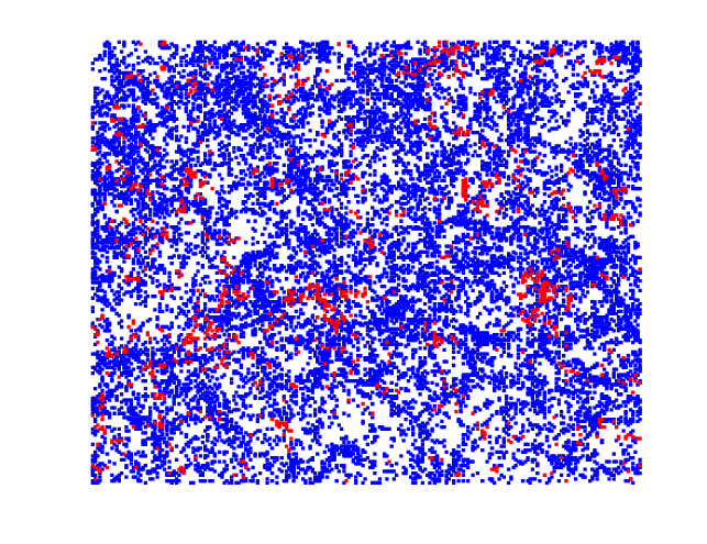
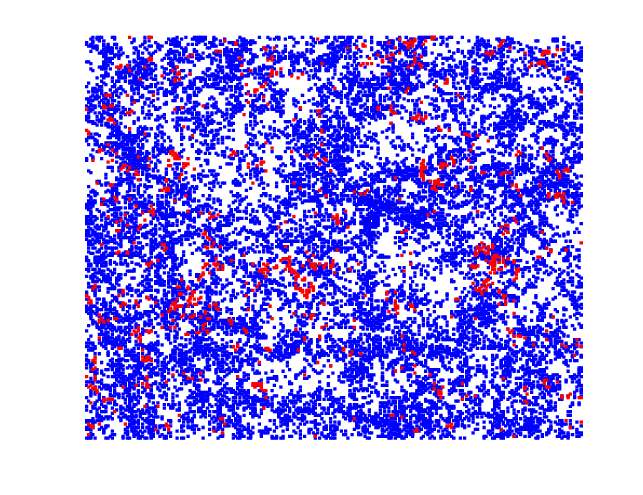
We emphasize that one can measure the line cross power spectrum from galaxies which are too faint to be seen individually over detector noise. Hence, a measurement of the line cross power spectrum can provide information about the total line emission from all of the galaxies which are too faint to be directly detected. One possible application of this technique would be to measure the evolution of line emission over cosmic time to better understand galaxy evolution and the sources that reionized the Universe. Changes in the minimum mass of galaxies due to photoionization heating of the intergalactic medium during reionization could also potentially be measured [1].
Here we use cosmological simulations to test the feasibility of measuring the galaxy line cross power spectrum. We create synthetic data sets for two hypothetical instruments, one on the Space Infrared Telescope for Cosmology an Astrophysics (SPICA) and the other consisting of a pair of ground based radio telescopes optimized to measure CO(1-0) and CO(2-1) emission from high redshifts. We test how well the cross power spectrum can be measured and find agreement with the analytical expectation derived in [1]. However there are some additional complications. Small -modes along the line of sight which are contaminated during the foreground removal process must be discarded, increasing the statistical uncertainty on large spatial scales. Additionally, when masking out contaminating emission lines from bright foreground galaxies one must be careful not to introduce a spurious correlation between the data sets being cross correlated.
The paper is organized as follows. In 2 we describe the methods used in this paper. This includes a brief review of the galaxy line cross power spectrum, a description of the synthetic data sets, the details of the simulations, and a discussion of the steps involved in measuring the cross power spectrum. In 3 and 4 we present our results for the SPICA example and the CO(1-0) and CO(2-1) telescopes, respectively. Finally, we discuss and summarize our conclusions in 5. Throughout, we assume a CDM cosmology with , , , , and , [12].
II Method
II.1 Galaxy line cross power spectrum
First, we briefly review the galaxy line cross power spectrum. For a more complete discussion, see Visbal Loeb (2010) [1]. We assume that emission is measured both as a function of angle on the sky and observed wavelength. If one fits a smooth function of wavelength along each direction on the sky and subtracts it from the data, one obtains the fluctuations from the average signal as a function of angle and wavelength: . There is a one to one correspondence between angular position and wavelength and spatial position for emission in a particular line. For convenience we use comoving coordinates at the location of the target galaxies instead of angle and wavelength. The fluctuations at a particular location results from a number of different sources,
| (1) |
which include contributions from the target galaxies we wish to cross correlate, detector noise, and emission in different lines from galaxies at different redshifts which we refer to as “bad line” emission. One can cross correlate the fluctuations in two different lines from the same galaxies. We define the line cross correlation function as,
| (2) |
where subscripts denote different lines being cross correlated. The center of the survey volume is denoted by , is the distance from the center in the first set of fluctuations, and is the distance from the center in the second set of fluctuations.
Because the noise fluctuations in the two different data sets are uncorrelated and galaxies seen in different bad lines will have very large separations and thus be essentially uncorrelated we are only left with contributions from the target galaxies. On large scales we can make the assumption that line fluctuations due to galaxy clustering are given by , where is the average target line signal, is the luminosity weighted average galaxy bias, and is the cosmological over-density at a location . It follows that,
| (3) |
where is the cosmological matter correlation function and the subscript numbers denote the different lines being cross correlated.
The line cross power spectrum is then defined as the Fourier transform,
| (4) |
where is the shot-noise power spectrum due to the discrete nature of galaxies.
An unbiased estimator for the cross power spectrum is given by the product of the Fourier transforms of the data sets,
| (5) |
where is the volume of the survey and the superscripts denote the different lines being cross correlated. The Fourier amplitude is given by,
| (6) |
Here is a window function that is constant over the survey volume and zero at all other locations. It is normalized such that, .
The root mean square (RMS) error in a measurement of the cross power spectrum at one particular -value is given by [1],
| (7) |
where and are the total power spectrum corresponding to the first line and second line being cross correlated. Each of these includes a term for the power spectrum for each of the bad lines, the target line, and detector noise (see Appendix A of Ref. [1]). When averaging nearby values of the power spectrum this error goes down by a factor of , where is the number of statistically independent -values at which the power spectrum is measured.
II.2 Synthetic data set
In order to test the feasibility of measuring the line cross power spectrum we create synthetic data sets for instruments measuring both spatial and spectral information. Our goal is to produce a realization of the light from all galaxies as a function of angular position and observed wavelength on a patch of the sky. We create these data with a cosmological dark matter simulation (described in detail below). From the simulation we construct a light cone which has the distribution of dark matter halos which would be observed today in the volume corresponding to an angular patch on the sky out to a redshift of .
A simple prescription is used to associate galaxies with the dark matter halos from our simulation. We assign each galaxy a spectrum and assume that its intensity scales with star formation rate (SFR). The SFR versus halo mass relation is determined by matching comoving density with observed UV luminosity functions [14, 15, 13, 16, 17].
We assume that galaxies are found in dark matter halos above a minimum mass, . After reionization represents the threshold for assembling heated gas out of the photo-ionized intergalactic medium, corresponding to a minimum virial temperature of [18]. We assume that reionization was completed by a redshift of . In all of the examples presented below, is set to correspond to this post-reionization requirement.
The larger dark matter halos in our simulation may host multiple galaxies. To incorporate this effect in our synthetic data we have used a simple prescription for the halo occupation distribution. Following Ref. [19] for the distribution of dark matter sub-halos, we consider two different types of galaxies: central and satellite. We assume that the distribution of central galaxies is a step function: above we assume each halo has one galaxy at its center. We then assume that there are a number of satellite galaxies given by a Poisson distribution with a mean of , here , and at ; at ; and at . We distribute these galaxies randomly, but weighted by an NFW profile, throughout the larger host dark matter halo. We treat the central and satellite galaxies as independent in assigning star formation rates to them as explained below. We associate half of the total halo mass to the central galaxy halos and split the remainder of the mass equally to all of the satellite galaxy halos.
After relating galaxies to dark matter halos in the simulation we produce a spectrum for each galaxy. For the continuum, we take the measured spectral energy distribution of M82 and scale it with the SFR [20]. The results are insensitive to the particular choice of galaxy continuum, as it is removed in the fitting and subtraction stage of the data analysis, as discussed below.
In order to estimate the amplitude of line emission fluctuations we assume a linear relationship between line luminosity, , and star formation rate, , , where is the ratio between SFR and line luminosity for a particular line. This is similar to existing relations in different bands (see Ref. [21]) and was used in the past to estimate the strength of the galactic lines we consider [22]. The values for relevant lines are shown in Table 1. For the first 7 lines, we use the same ratios, , as in Ref. [22] which were calculated by taking the geometric average of the ratios from an observational sample of lower redshift galaxies [23]. The other lines have been calibrated based on the galaxy M82 [24]. We assign a width to the lines based on the circular virial velocity of the dark matter halos, but the results are mostly insensitive to this choice for the spectral resolutions we consider in our examples. This is because the majority of the signal comes from lines which are spectrally unresolved.
For the results presented below we have made the simplification that all galaxies have the same R value for each emission line. Even if there is random scatter in the R values in each galaxy, the line cross power spectrum will remain unchanged. This scatter will behave essentially like detector noise with intensity that is non-uniform across the data cube.
| Species | Emission Wavelength[m] | R[] |
|---|---|---|
| CII | 158 | |
| OI | 145 | |
| NII | 122 | |
| OIII | 88 | |
| OI | 63 | |
| NIII | 57 | |
| OIII | 52 | |
| 12CO(1-0) | 2610 | |
| 12CO(2-1) | 1300 | |
| 12CO(3-2) | 866 | |
| 12CO(4-3) | 651 | |
| 12CO(5-4) | 521 | |
| 12CO(6-5) | 434 | |
| 12CO(7-6) | 372 | |
| 12CO(8-7) | 325 | |
| 12CO(9-8) | 289 | |
| 12CO(10-9) | 260 | |
| 12CO(11-10) | 237 | |
| 12CO(12-11) | 217 | |
| 12CO(13-12) | 200 | |
| CI | 610 | |
| CI | 371 | |
| NII | 205 | |
| 13CO(5-4) | 544 | 3900 |
| 13CO(7-6) | 389 | 3200 |
| 13CO(8-7) | 340 | 2700 |
| HCN(6-5) | 564 | 2100 |
We use observed UV luminosity functions ([14, 15, 13, 16, 17]) of galaxies to calibrate the SFR assigned to dark matter halos with an abundance matching technique. Given the observed luminosity functions, we determine the number density of galaxies as a function of SFR through the relation,
| (8) |
where is given by at a rest frame wavelength of . This assumes a Salpeter initial mass function from and a constant . The relationship between halo mass, , and SFR at some particular mass, is found from the relation . Here is the number density of dark matter halos above mass in our simulation and is the number density of galaxies implied by the UV luminosity function above the SFR value, . This procedure is carried out in a number of different redshift bins which cover our entire light cone. As a simple correction for attenuation due to dust we increase the SFR of all halos in each redshift bin by a factor which sets the global SFR equal to that given in Ref. [13] (the blue solid curve in Figure 10 of Ref. [13]). In the highest redshift bin we do not apply any dust correction. The particular parameters used for the abundance matching procedure are listed in Table 2.
| Ref. | ||||
|---|---|---|---|---|
| 0.0-0.5 | 4.07 | -18.05 | -1.21 | [14] |
| 0.5-1.0 | 3.0 | -19.17 | -1.52 | [15] |
| 1.0-1.5 | 1.26 | -20.08 | -1.84 | [15] |
| 1.5-2.0 | 2.3 | -20.17 | -1.60 | [15] |
| 2.0-2.7 | 2.75 | -20.7 | -1.73 | [13] |
| 2.7-3.4 | 1.71 | -20.97 | -1.73 | [13] |
| 3.4-4.5 | 1.3 | -20.98 | -1.73 | [16] |
| 4.5-5.5 | 1.0 | -20.64 | -1.66 | [16] |
| 5.5-6.5 | 1.4 | -20.24 | -1.74 | [16] |
| 6.5-10.5 | 0.86 | -20.14 | -2.01 | [17] |
Finally, we add detector noise and bright astronomical foreground and background emission. For the examples below we include both the CMB and emission from dust in our galaxy. The dust emission is treated as a black body with a emissivity scaled to match the background radiation measured by COBE FIRAS in the faintest area on the sky [25]. In Figure 2, we illustrate the different components which make up our data sets.

II.3 Simulations
To create our synthetic data we simulate the light cone of dark matter in a 100100 arcmin2 angular patch of the sky out to high redshift. We use a particle-multi-mesh N-body code to evolve the dark matter distribution [26]. The simulation outputs are then stacked along the line of sight out to z = 10.
For most of our light cone, we use an N-body simulation with 20483 dark matter particles on an effective mesh with 76803 cells in a comoving box with a length of 200 on a side. This length is sufficient to cover the field of view out to the highest redshifts of interest. For low redshifts (), we use a second larger simulation to improve the sample variance of large halos. This simulation also contains 20483 dark matter particles and a mesh of 76803 cells, but has a length of 400 on each side of the box. In both simulations we identify dark matter halos using a spherical overdensity algorithm. This is done by examining snapshots taken every 20 Myr and 40 Myr in the 200 and 400 simulations respectively.
The light cone is constructed from a series of redshift zones, each zone spanning one comoving box length. Each zone is constructed from several redshift shells of thickness corresponding to a time interval of 20 or 40 Myr depending on the box size. The shells are stacked in a continuous fashion, but the zones are randomized to eliminate any very long artificial structure. This produces a discontinuity across zone boundaries. We are careful to only measure the power spectrum within one zone for our examples to avoid any problems associated with this discontinuity.

II.4 Cross power spectrum measurement
Measuring the cross power spectrum consists of three main steps:
1. Fitting a smooth function of wavelength to each pixel and subtracting it away (note that we term each line of sight on the sky a “pixel” and each spectral component of the 3D data cube a “voxel”).
2. Masking out voxels with bright bad line emission.
3. Taking the product of the Fourier modes to estimate the power spectrum and then averaging in spherical shells in -space.
We discuss these in turn. The fitting stage is necessary because we seek to measure only the signal coming from line emission and our data contains signal from both galaxy continuum emission as well as bright astrophysical foregrounds and backgrounds. Since these other sources vary slowly in the spectral direction we can remove them by fitting a smooth function of wavelength to each pixel on the sky and subtracting it. This is the same procedure which has been discussed extensively in the context of cosmological measurements of 21cm radiation from neutral hydrogen [6, 7, 8, 9, 10].
More specifically, with our data sets we fit a polynomial in wavelength to the spectrum in each pixel and then subtract it away. This removes the foregrounds and galaxy continuum, as well as some large scale fluctuations in line emission along the line of sight. In order to minimize loss of the line signal we do not include voxels in our fit which contain bright line emission. We do this by an iterative fit: we fit once to remove the foregrounds and identify the bright voxels and then fit again excluding them.
There will necessarily be some signal lost on large scales as a result of the fitting and subtraction stage. Fortunately as discussed in Ref. [6], if we decompose our signal into Fourier modes, the lost signal is only from small -modes (corresponding to long wavelengths) along the line of sight. If we exclude these corrupted -modes in step 3 of measuring the cross power spectrum, we still have an unbiased estimation of the cross power spectrum without subtraction losses. Note that throwing away the low -modes does have a price. Since there are fewer statistical samples of modes this procedure increases the variance of power spectrum measurements on large scales. Because we wish to minimize the number of these corrupted modes, we fit with the lowest order polynomial which leaves no significant residual foregrounds.
After we have subtracted away the foreground and continuum emission it is necessary to remove voxels with very bright bad line emission. This is necessary because even though line emission from bright foreground galaxies does not bias our measurements of the power spectrum it does increase the error of our measurements due to the contribution in Eq. (7).
The masking procedure must be done carefully in order to not introduce spurious correlations between the two data sets being cross correlated. For example, if one simply sets all voxels above some threshold signal equal to zero, a spurious change to the cross power spectrum is introduced (see Fig. 5). This is because the location of the brightest voxels (mainly due to contaminating bright foreground galaxies) are correlated with the distribution of target line emission. The signal from the bad lines and the target lines overlap so that bright bad lines which appear in the data at locations of over-densities in the target lines are more likely to be above the removal threshold. Thus, the bad lines left after masking in one data cube will be anti-correlated with the target lines in the other cube. This causes the measured cross power spectrum to be lower than what would be measured from the target lines alone.
In order to avoid this type of complication one can mask out voxels in a way which is uncorrelated with the target line emission being measured. This can be done by identifying individual bright sources instead of just removing the brightest voxels in the data. The voxels with bright contaminating lines can then be set to zero. These sources could be identified by looking at a series of different wavelengths and identifying them with multiple lines. Entirely different surveys could also be used to determine where contaminating lines from bright foreground galaxies will appear and be removed. In our examples below, we assume that all of the galaxies which emit lines brighter than five times the RMS detector noise can be identified directly. When setting the masked voxels to zero we treat this as a change in the window function, , which appears in Eq. (6). We normalize this new window function such that .
In the final step, we take the discrete Fourier transform of the two 3D data cubes being cross correlated. The estimation of the power spectrum at some particular value is then given by the real part of the product of the survey volume, the Fourier mode of one data set, and the complex conjugate of the same Fourier mode in the other data set. This is equivalent to Eq. (5). Finally, we break -space into spherical shells with uniform thickness in . We then take the average estimated power spectrum of all the modes contained within each shell. As discussed above, we do not include low -modes along the line of sight which have been contaminated during the fitting and subtraction stage. Specifically, we do not include -modes which have a component along the line of sight smaller than, , the lowest value for which there is no significant contamination. In the examples below we find that for there is no significant loss of power due to the foreground removal process.
III SPICA
III.1 Instrument
We consider two different examples of instruments and lines which could be used to measure the galaxy line cross power spectrum. In our first example, we envision an instrument on the planned Space Infrared Telescope for Cosmology and Astrophysics (SPICA) [27]. SPICA is a 3.5 meter space-borne infrared telescope planned for launch in 2017. It will be cooled below K, providing measurements which are orders of magnitude more sensitive than those from current instruments. We consider an instrument based on the proposed high performance spectrometer -spec (H. Moseley, private communication 2009). This instrument will provide background limited sensitivity with wavelength coverage from . A number of -spec units will be combined to record both spatial and spectral data in each pointing, which will be perfectly suited for intensity mapping. We assume that spectra for diffraction limited beams can be measured simultaneously with a resolving power of .

| OI(63 m) | OIII(52 m) | |
| Average Line Signals () | ||
| Fraction of Voxels Masked | 0.097 | 0.11 |
| RMS Detector Noise | ||
| Brightness of CMBDust | ||
| Bad line PowerNoise Power (Mpc) | 6.5 | 8.1 |
| Bad line PowerNoise Power (Mpc) | 1.4 | 1.7 |
| Cross Power SN per -mode (Mpc) | 0.17 | |
| Cross Power SN per -mode (Mpc) | 0.14 |

III.2 Results
We use the simulation described above to create a synthetic data set and measure the cross power spectrum with the SPICA/-spec instrument. We cross correlate OI(63 m) and OIII(52 m) from galaxies at a redshift of . We assume the data covers a square on the sky which is 1.7 degrees across (corresponding to 250 Mpc) and a redshift range of (corresponding 280 Mpc). We assume a total integration time of seconds spread uniformly across this survey area.
In Figure 4, we show that using the procedure described above we can accurately measure the cross power spectrum. We show both the cross power spectrum of the emission from the target lines alone as well as that which is recovered when bad lines, detector noise, and foregrounds are included. The error in measuring the power spectrum is consistent with the analytical prediction derived in Ref. [1]. The details introduced in our simulation and measurements, such as removing the foregrounds and masking out bright foreground galaxies, does not bias our estimate of the power spectrum or increase the uncertainty implied by Eq. (7). Other details of this example are presented in Table 3.
In Figure 5, we show the effects on the measured cross power spectrum of masking out all bright voxels. We have plotted the power spectrum from the target lines alone and also with the bad lines using the same mask in both cases. Clearly, the anti-correlation between the masked bad lines and the target lines in the other data set described above has biased the cross power spectrum measurement.
We find that increasing the sky coverage (i.e. shorter integrations for each pointing on the sky, but larger sky coverage) increases our errors in the power spectrum. This is due to our assumptions about masking bright bad lines. As the survey becomes wider the detector noise goes up and the increased number of bright bad lines which are not masked increases the errors on the power spectrum. One would not want to go much deeper over a smaller patch of sky than we consider, because we are already masking roughly of each data cube. Without using the increased sensitivity to remove more of the bright bad lines, going deeper and shallower would increase the noise in the power spectrum due to increased sample variance.
If the mask were not dependent on the integration time (e.g. obtained from a different survey of foreground galaxies) it is straight forward to determine in a given time what the optimal sky coverage is for measuring power on a particular scale. Minimizing Eq. (7) with respect to time integrated per pointing, holding the total observation time fixed, one finds that the optimal coverage sets . The product of the detector noise power spectra equals the sum of the sample variance contribution to the power spectrum uncertainty.

| CO(1-0) | CO(2-1) | |
|---|---|---|
| Average Line Signals () | 0.1K | 0.094K |
| Fraction of Voxels Masked | 0.0 | 0.015 |
| RMS Detector Noise | 1.0K | 0.7K |
| Bad line PowerNoise Power (Mpc) | 0.0 | 7.0 |
| Bad line PowerNoise Power (Mpc) | 0.0 | 1.5 |
| Bad line PowerNoise Power (Mpc) | 0.0 | 0.5 |
| Cross Power SN per -mode (Mpc) | 0.24 | |
| Cross Power SN per -mode (Mpc) | 0.12 | |
| Cross Power SN per -mode (Mpc) | 0.05 |
IV Intensity mapping CO(1-0) and CO(2-1)
As another example we consider intensity mapping the cross correlations between CO(1-0) and CO(2-1) at high redshifts with a dedicated instrument currently being planned (J. Bowman 2011, private communication). Other similar instruments are currently being planned (G. Bower 2011, private communication). This observation consists of two telescopes: a 20 meter dish and a 10 meter dish to observe CO(1-0) and CO(2-1) respectively. Each of these telescopes can simultaneously observe 3 of the sky with angular resolution set by the beam size (3.5-5 arcmin at ). We assume a spectral resolution of . While the actual instrument will have a higher resolution this is sufficient to measure fluctuations on the scales we consider. To determine the detector noise we use the radiometer equation [28],
| (9) |
where is the system temperature which we have assumed to be 30K, is the integration time which we have assumed is s, and the factor of appears in the denominator because the intensity will be mapped from dual polarization. We create a synthetic data set for this instrument centered at and the recovered cross power spectrum is shown in Figure 6. We summarize some other properties of this simulated measurement in Table 4.
V Discussion and conclusions
By cross correlating emission in different spectral lines from the same galaxies, it is possible to measure their clustering. This clustering, quantified by the line cross power spectrum, can be measured for galaxies which are too faint to detect individually, but which can be observed in aggregate due to their large numbers [1].
In this paper, we have shown that the line cross power spectrum can be accurately measured with future instruments, based on synthetic data created using cosmological dark matter simulations. We produced our synthetic data by associating dark matter halos with galaxies and assigning each a spectrum. The continuum was generated by scaling that of M82 with the SFR in each halo and line emission was set by calibrating with lower redshift galaxies. The SFR was computed for halos with an abundance matching technique calibrated to observations of galaxy UV luminosity functions. Our synthetic data also included detector noise and bright emission due to astrophysical foregrounds and backgrounds such as that from dust in our galaxy and the CMB. Even if our simple prescription deviates somewhat from reality, it still illustrates our main point, that whatever the underlying power spectrum of emission from galaxies is, it can be measured with the accuracy predicted analytically by Eq. (7). It is reassuring that the complications addressed in our simulations such as removal of bright astrophysical foregrounds and masking out bright bad line emission do not hinder measurement of the power spectrum compared to the analytic expectations from Ref. [1].
Measuring the line cross power spectrum consists of three main steps. First, a smooth function such as a polynomial is fit to each pixel on the sky and subtracted from the data to remove smooth foregrounds and the continuum emission from galaxies. Next, bright voxels are masked out. One must be careful in the masking technique as it is possible to introduce spurious correlations if the masks are correlated with the target lines which appear in both data cubes. This can be avoided if bright sources are found individually at high significance and the corresponding voxels with bright contaminating lines are set to zero. Finally, the data is Fourier transformed and then the power spectrum is averaged in spherical shells. Modes corresponding to long wavelengths along the line of sight are not included, because they are contaminated during the fitting and subtraction step.
We find that the line cross power spectrum can be measured with the accuracy predicted analytically by Eq. (7), derived in Ref. [1]. In particular, we tested two hypothetical instruments, an instrument mounted on SPICA and a pair of large ground based telescopes designed to measure the emission of CO(1-0) and CO(2-1). Though not included in our examples, it would also be valuable to measure emission from more than two different lines from the same redshifts. This could improve statistics and allow determination of the ratio of line emission in different lines by taking the ratio of different cross power spectra.
Our results suggest that cross correlating galaxy line emission is a promising technique for studying high redshift galaxies. It will enable one to measure the evolution of the total line signal from all galaxies at a particular redshift, even those that are too faint to be resolved individually. This could reveal details about the evolution of galaxies’ properties such as SFR density or average metallicity. It may also be possible to use these observations to study the history of cosmic reionization, both by estimating the ionizing flux from faint galaxies and by looking for a sharp change in signal versus redshift due to the change in the minimum mass of halos which host galaxies.
VI Acknowledgments
We thank Judd Bowman for helpful discussions. This work was supported in part by NSF grant AST-0907890 and NASA grants NNA09DB30A and NNX08AL43G (for A.L.).
References
- [1] E. Visbal and A. Loeb, JCAP 11, 16 (2010), eprint 1008.3178.
- [2] Y. Gong, A. Cooray, M. B. Silva, M. G. Santos, and P. Lubin, The Astrophysical Journal Letters 728, L46+ (2011), eprint 1101.2892.
- [3] C. L. Carilli, The Astrophysical Journal Letters 730, L30+ (2011), eprint 1102.0745.
- [4] A. Lidz, P. Oh, S. Furlanetto, O. Dore, T. Chang, and J. Pritchard, (in prep) (2011).
- [5] J. Binney and M. Merrifield, Galactic astronomy (Princeton University Press, 1998).
- [6] N. Petrovic and S. P. Oh, ArXiv e-prints (2010), eprint 1010.4109.
- [7] M. F. Morales, Astrophys. J. 619, 678 (2005).
- [8] X.-M. Wang, M. Tegmark, M. Santos, and L. Knox, Astrophys. J. 650, 529 (2006).
- [9] M. McQuinn, O. Zahn, M. Zaldarriaga, L. Hernquist, and S. R. Furlanetto, Astrophys. J. 653, 815 (2006).
- [10] A. Liu, M. Tegmark, J. Bowman, J. Hewitt, and M. Zaldarriaga, Mon. Not. Roy. Astron. Soc. 398, 401 (2009), eprint arXiv:astro-ph/0903.4890.
- [11] A. Liu and M. Tegmark, ArXiv e-prints (2011), eprint 1103.0281.
- [12] E. Komatsu, K. M. Smith, J. Dunkley, C. L. Bennett, B. Gold, G. Hinshaw, N. Jarosik, D. Larson, M. R. Nolta, L. Page, et al., ArXiv e-prints (2010), eprint arXiv:astro-ph/1001.4538.
- [13] N. A. Reddy and C. C. Steidel, Astrophys. J. 692, 778 (2009), eprint 0810.2788.
- [14] S. Arnouts, D. Schiminovich, O. Ilbert, L. Tresse, B. Milliard, M. Treyer, S. Bardelli, T. Budavari, T. K. Wyder, E. Zucca, et al., The Astrophysical Journal Letters 619, L43 (2005), eprint arXiv:astro-ph/0411391.
- [15] P. A. Oesch, R. J. Bouwens, C. M. Carollo, G. D. Illingworth, D. Magee, M. Trenti, M. Stiavelli, M. Franx, I. Labbé, and P. G. van Dokkum, The Astrophysical Journal Letters 725, L150 (2010), eprint 1005.1661.
- [16] R. J. Bouwens, G. D. Illingworth, M. Franx, and H. Ford, Astrophys. J. 670, 928 (2007), eprint 0707.2080.
- [17] R. J. Bouwens, G. D. Illingworth, P. A. Oesch, I. Labbe, M. Trenti, P. van Dokkum, M. Franx, M. Stiavelli, C. M. Carollo, D. Magee, et al., ArXiv e-prints (2010), eprint 1006.4360.
- [18] S. Wyithe and A. Loeb, Nature 441, 332 (2006).
- [19] A. V. Kravtsov, A. A. Berlind, R. H. Wechsler, A. A. Klypin, S. Gottlöber, B. Allgood, and J. R. Primack, Astrophys. J. 609, 35 (2004), eprint arXiv:astro-ph/0308519.
- [20] L. Silva, G. L. Granato, A. Bressan, and L. Danese, Astrophys. J. 509, 103 (1998).
- [21] R. C. Kennicutt, Jr., Annual Review of Astronomy and Astrophysics 36, 189 (1998), eprint arXiv:astro-ph/9807187.
- [22] M. Righi, C. Hernández-Monteagudo, and R. A. Sunyaev, Astronomy and Astrophysics 489, 489 (2008), eprint arXiv:astro-ph/0805.2174.
- [23] S. Malhotra, M. J. Kaufman, D. Hollenbach, G. Helou, R. H. Rubin, J. Brauher, D. Dale, N. Y. Lu, S. Lord, G. Stacey, et al., Astrophys. J. 561, 766 (2001), eprint arXiv:astro-ph/0106485.
- [24] P. Panuzzo, N. Rangwala, A. Rykala, K. G. Isaak, J. Glenn, C. D. Wilson, R. Auld, M. Baes, M. J. Barlow, G. J. Bendo, et al., Astronomy and Astrophysics 518, L37+ (2010), eprint 1005.1877.
- [25] D. J. Fixsen, E. Dwek, J. C. Mather, C. L. Bennett, and R. A. Shafer, Astrophys. J. 508, 123 (1998), eprint arXiv:astro-ph/9803021.
- [26] H. Trac and U. Pen, New Astronomy 11, 273 (2006), eprint arXiv:astro-ph/0402444.
- [27] B. Swinyard, T. Nakagawa, P. Merken, P. Royer, T. Souverijns, B. Vandenbussche, C. Waelkens, P. Davis, J. Di Francesco, M. Halpern, et al., Experimental Astronomy 23, 193 (2009).
- [28] T. L. Wilson, K. Rohlfs, and S. Hüttemeister, Tools of Radio Astronomy (Springer-Verlag, 2009).