Some necessary conditions for allowing the PQ scale
as high as in SUSY models
with an axino or neutralino LSP
Abstract:
We examine some conditions which are needed to allow the Peccei-Quinn scale () as high as the SUSY GUT scale ( in the context of the PQMSSM with either an axino or a neutralino LSP. The main problem in non-SUSY models with is the generation of an overabundance of axion dark matter () due to vacuum misalignment. We show that once all the components of the axion supermultiplet are included, the upper limit on can be evaded due to large entropy injection from saxion decays. This large entropy injection also dilutes all other quasi-stable relic densities, naturally evading the BBN constraints and solving the gravitino problem. We find that can be allowed by relic density/BBN constraints provided that the saxion mass TeV, the initial saxion field value is of order of the PQ scale and the initial axion mis-alignment angle . These restrictions can be considerably loosened for GeV. The allowed range for the re-heat temperature () is strongly dependent on the nature of the LSP. For the axino LSP, GeV, while for neutralino LSP any value is allowed. In the latter case, can be more easily accommodated than in the axino LSP scenario. For in SUSY models, the dark matter abundance should be dominated by axions, albeit with mass eV, far below the region currently probed by experiment.
Keywords:
Supersymmetry Phenomenology, Supersymmetric Standard Model, Dark Matter1 Introduction
The strong problem remains one of the central puzzles of QCD which evades explanation within the context of the Standard Model. The crux of the problem is that an additional violating term in the QCD Lagrangian of the form11 1 Here is the gluon field strength tensor and its dual. ought to be present as a result of the t’Hooft resolution of the problem via instantons and the vacuum of QCD [1]. Here, actually consists of two terms: one from QCD and one from the electroweak quark mass matrix. The experimental limits on the neutron electric dipole moment however constrain [2]. Explaining why the sum of these two terms should be so small is the essence of the strong problem[3].
An extremely compelling solution proposed by Peccei and Quinn [4] is to hypothesize an additional global symmetry, which is broken at some mass scale GeV. A consequence of the broken PQ symmetry is the existence of a pseudo-Goldstone boson field: the axion [5]. The low energy Lagrangian then includes the interaction term
| (1) |
where , is the QCD coupling constant and is the model-dependent color anomaly factor. (From here on we assume , but all our results can be extended to any value with the replacement .) Since is dynamical, the entire -violating term settles to its minimum at zero, thus resolving the strong problem. A consequence of this very elegant mechanism is that a physical axion field should exist, with axion excitations of mass[6]
| (2) |
Due to its tiny mass, the interactions of the axion field need to be strongly suppressed– GeV– otherwise they would have a strong impact on low energy physics and astrophysics[7], such as too rapid cooling of stars and supernovae. On the other hand, under some model assumptions (see Sec. 3.1 below), the axion relic density bound requires GeV. As a consequence a new physics scale much larger than the electroweak scale () has to be introduced into the Standard Model[8, 9]. This results in large radiative corrections to the Higgs mass, which then requires a large amount of fine-tuning to stabilize the EW scale. This leads to the well known hierarchy problem.
So far, one of the most compelling solutions to naturally stabilize the EW scale is supersymmetry (SUSY), which reduces quadratic divergences to merely logarithmic, and ameliorates the fine-tuning problem[10]. The supersymmetric version of the Standard Model (MSSM) also has other compelling features, such as viable Dark Matter (DM) candidate(s) and unification of the gauge coupling constants at GeV. In order to accomodate the PQ solution in the MSSM, it is necessary to postulate the existence of new superfields carrying PQ charge. Although this extension of the MSSM can be realized in a number of ways, we will call the resulting weak-scale effective theory the PQMSSM.
It has been noticed early on[11] that the PQ scale falls within the desired range for the SUSY breaking scale () in gravity-mediated SUSY breaking models:
| (3) |
where is the gravitino mass and is the reduced Planck mass. As a result, several models have been proposed[11, 12, 13] to connect the SUSY and PQ breaking scales. This can be achieved if the axion supermultiplet has tree level interactions with the hidden sector responsible for breaking SUSY.
However, once a grand unified theory is assumed, the symmetry can appear as an accidental global symmetry of the theory, as naturally occurs in several SUSY GUTS[14]. In this case, will naturally be of order and will strongly violate its GeV upper limit. It is possible to protect from obtaining contributions, either by breaking the PQ symmetry at a lower scale or artificially suppressing the vacuum expectation value of the axion supermultiplet. Nonetheless such mechanisms always require the introduction of new superfields or fine-tuned parameters only for this purpose.
String theory has emerged as an attractive ultraviolet complete theory which can easily incorporate axion-like fields as elements of anti-symmetric tensors[15]. Many of the would-be axions become massive, while the remaining light fields obey a global PQ symmetry. A survey of a variety of string models[16, 17] indicates that while PQ symmetry is easy to generate in string theory, the associated PQ scale tends to occur at or near the GUT scale rather than some much lower intermediate scale. This is in apparent conflict with the simple limits on from overproduction of dark matter as discussed above.
One solution to the apparent conflict which allows for is to invoke a tiny initial axion mis-alignment angle . In this case, one must accept a highly fine-tuned initial parameter which might emerge anthropically.
An alternative solution was proposed in one of the original papers calculating the cosmic abundance of relic axions[18]: perhaps additional massive fields are present in the theory, whose late decays can inject substantial entropy into the universe at times after axion oscillations begin, but before BBN starts. In Ref. [18], it was proposed that the gravitino might play such a role. Several subsequent works have also explored the issue of dilution of (quasi)-stable relics via entropy injection[19, 20, 21, 22, 23, 24, 25, 26].
Therefore it is of interest to investigate under which conditions the PQ scale can be extended to the GUT scale, while avoiding the known experimental constraints. While this possibility has been suggested before[21, 23], we wish to explore this case using detailed calculations of particle production rates coupled with recent constraints arising from Big Bang nucleosynthesis (BBN). Here, we investigate the implications of from a phenomenological point of view. In order to keep our conclusions as general as possible we will avoid choosing a specific GUT theory or PQMSSM model whenever possible.
In Sec. 2, we will present the general features of PQMSSM cosmology used in our analysis and review several well known results for this model. We will then discuss the scenario in Sec. 3 and the case of a light axino LSP in Sec. 4. We will present the main difficulties associated with large values and show how they can be avoided in the PQMSSM framework. In Sec. 5, we discuss the scenario where , where the neutralino is assumed to be LSP. In several respects, this scenario is more appealing than the light axino LSP case. Section 6 summarizes our main results and discusses the implications of unifying the PQ and GUT scales. The appendices contain explicit formulae for evaluating the axion and neutralino relic abundances in radiation-, matter- and decaying-particle- dominated universes.
2 PQMSSM Phenomenology
In order to implement the PQ mechanism in supersymmetric theories, PQ charges have to be assigned to the MSSM fields and new PQ superfields must be introduced. The axion superfield is obtained from linear combinations of other elementary (non-MSSM) fields and is a singlet under the MSSM gauge group. Even though the full field content of the PQMSSM is highly model dependent, it must contain an axion supermultiplet composed of a complex scalar field () and a Majorana fermion (). The complex scalar field is usually divided into its axion () and saxion () components:
and the fermionic component is named axino.
Since the axion field is the pseudo-Goldstone boson, it is massless, except for anomalous corrections coming from the QCD chiral anomaly. For temperatures well above (the QCD chiral breaking scale), the axion is essentially massless, while for the QCD chiral anomaly induces a non-zero mass for the axion field. The temperature dependent axion mass is given by[27, 28]:
where , MeV and always refers to the thermal bath temperature.
In order to solve the strong CP problem, the axion field must have effective couplings to the gauge fields of the form shown in Eq. (1). Although other non-minimal interactions are possible, they are strongly model dependent and will be neglected here.
The supersymmetric version of Eq. (1) implies the following couplings for the saxion and axino fields:
| (4) |
In most models, the axino also couples to the gauge boson and gaugino:
| (5) |
where is a model dependent constant of order 1. Couplings between the saxion and axion, as well as between axinos and fermions-sfermions can also exist, but are model dependent.
If supersymmetry is unbroken, both the axino and saxion are degenerate with the axion field, hence massless, except for the tiny QCD anomaly contribution. However, once SUSY is broken the saxion field will receive a soft mass of order . On the other hand, being the fermion component of a chiral superfield, the axino remains massless at tree level. Nonetheless, the axino can receive loop corrections to its mass[29] of order eV, for . In this case the axino is the lightest supersymmetric particle (LSP) in the PQMSSM model. However, depending on the PQMSSM model, can also receive contributions from the supergravity potential[30]. In this case, the axino might remain as the LSP, or the lightest neutralino could be the LSP[31, 32], with . The case of a gravitino as LSP is considered in Ref. [33].
In the case of axino LSP, the can be long-lived due to its suppressed couplings to the axino; this has important cosmological implications. Assuming the minimal interactions of Eq’s. (4) and (5), we have the following decay rates:
| (6) | |||||
where is the bino component of the neutralino field in the notation of Ref. [10]. If the neutralino is the LSP, the axino will be long-lived instead. The decay rates for are given by the above equations with . However, if the axino is heavier than neutralinos or gluinos, new decay modes or open up. Since the decay rates for these are discussed in Ref.[32], we do not reproduce them here.
Due to the first interaction term in Eq. (4), the saxion decay width to is model independent, with decay width given by:
| (7) |
Saxions also decay to gluino pairs, but its width is always well below that to gluon pairs, as shown in Ref. [34]. The saxion might also decay directly into two axions. The decay width to axion pairs is given by:
| (8) |
where is a model dependent coupling. For our subsequent analysis, we will assume that the above decay mode is suppressed with respect to the one in Eq. (7); this suppression is common in models with universal soft SUSY breaking terms[35].
2.1 PQMSSM cosmology
The cosmology of PQMSSM models is very rich and has to be carefully examined. Here, we will assume that the PQ symmetry breaks before the end of inflation so as to avoid domain wall problems[36].
Due to their suppressed interactions, the axion, axino and saxion rapidly decouple from the thermal bath in the early universe or are already produced out of equilibrium, if the reheat temperature after inflation is smaller than the decoupling temperature[37]:
| (9) |
However, for the values of considered here ( GeV), the decoupling temperature is always above . Since we only consider the case where the PQ symmetry is broken before inflation ends (), we always have and axions, saxions and axinos are never in thermal equilibrium. In this case, the axion, saxion and axino thermal yields at are estimated as[38, 39, 35, 40]:
| (10) | |||||
where is the strong coupling constant at and we have used .
In an analogous way, gravitinos are thermally produced in the early universe with yield given by[41]:
| (11) |
where , , are the gauge couplings evaluated at and are the gaugino masses also evaluated at . To compute the gravitino yield we assume , since we only consider cases with TeV. However, most of our results are weakly dependent on this assumption. If entropy is always conserved from to , Eq’s. (10) and (11) are still valid at and can be used to compute the relic energy density today.
Besides being produced from scattering of particles in the thermal bath, the saxion and axion fields can also contribute to the energy density through coherent oscillations. For , the expansion rate of the universe is too large and suppresses any oscillations, which only start at . The axion and saxion oscillation temperatures are then defined by[42, 43]:
| (12) |
where is the temperature dependent axion mass. In most regions of the PQMSSM parameter space, we have GeV and GeV for a TeV scale saxion.22 2 For saxion oscillation in a radiation dominated universe, . For reheat temperatures smaller than , the saxion field starts to oscillate during the inflaton-dominated universe and will be diluted due to the inflaton entropy injection. In this case, the saxion coherent oscillation density increases with until , where it then becomes independent. The specific details of the transition from the static to the oscillating regime are strongly model dependent, but can be parametrized by an arbitrary initial field amplitude. If the axion oscillation starts in a radiation dominated universe, for , the axion and saxion coherent oscillation Yields are given by33 3 Our saxion Yield expressions differ from Ref.[35] by a numerical factor because they assume the saxion field begins to oscillate at while we take to be consistent with the usual axion oscillation condition.:
where[28] and and are the initial saxion and axion field amplitudes and are expected to be of order .
From the above expressions we see that for most purposes the PQMSSM parameter space can be restricted to:
| (19) |
For simplicity, we take as in the DFSZ[9] axion model or in the KSVZ[8] model with PQ quark charges .
2.1.1 Early saxion dominated universe
Due to the small couplings of the axion supermultiplet, its components decouple from the thermal bath at very high temperatures. For temperatures below for thermally produced saxions or below for coherent oscillating saxions, the energy density of the saxion field scales as . Since the radiation energy density scales as , if the saxion is sufficiently long-lived, it will dominate the energy density of the universe. Defining and as the temperatures at which the saxion dominated era starts and ends, respectively, we have:
| (20) | |||||
| (21) |
where is the saxion decay rate given by Eq. (6) and is the reduced Planck mass. If , the saxion decays before dominating the energy density and its effects can be safely neglected44 4 If the saxion field has a large branching ratio into axions, its decays contribute to a hot DM component even for . However, as mentioned in Sec. 2, here we assume .. However, if , the universe becomes matter (saxion) dominated for . At most of the saxions have decayed and the radiation dominated era resumes.
Fig. 1 shows as a function of the reheat temperature for TeV, and , and GeV. As we can see, increases with until , when the saxion starts to oscillate after inflation. In this regime, the saxion Yield and hence becomes independent of . From Fig. 1, we see that for GeV and TeV, can be as large as GeV.

In Fig. 2, we plot as a function of for , and GeV. We see that can span a wide range of values, with MeV for a sub-TeV saxion and GeV. However, if MeV, entropy will be injected during the neutron freeze-out and the neutron-proton ratio will be significantly diluted. Since the success of BBN predictions strongly constrains the neutron-proton ratio to the value obtained in a radiation dominated universe, we must have MeV in order to have a neutron freeze-out during the radiation dominated era, thus preserving the successful BBN predictions. As shown in Fig. 2, this requires TeV for GeV. This bound can be softened by including additional model-dependent saxion decays such as .

Once starts to decay, entropy will be injected and effectively dilute all other relic densities already decoupled from the thermal bath, such as axinos, axions, gravitinos and possibly neutralinos. If the decoupling happens before the saxion dominated era (this is always the case for thermal axions, axinos and gravitinos), the dilution factor () is approximately given by[44]:
| (22) |
where is the number of relativistic degrees of freedom averaged over the saxion decay period, which we approximate by . Fig. 3 shows contours of values in the vs plane. We see that, for and GeV, values of larger than are easily obtained.
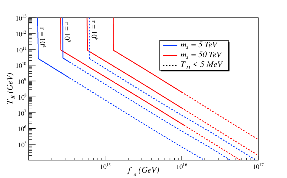
However, if the decoupling from the thermal bath happens during the saxion dominated period, as it might be the case for neutralinos or for the beginning of axion oscillation, the dilution factor will be modified due to the faster expansion rate during the saxion dominated phase. As a result, the neutralino freeze-out temperature () and the axion oscillation temperature () will be modified, if .
Finally, if the decoupling (or axion oscillation) happens after the saxion decay, there will be no dilution. In summary, for the case of an early saxion dominated universe (), we have:
| (23) |
where represents the axion, axino, gravitino or neutralino relic density, is the corresponding relic density in a radiation dominated (RD) universe (such as when ), is the decoupling or axion oscillation temperature and marks the transition between the matter dominated phase (MD) and the decaying particle dominated phase (DD) and can be approximated by (see Appendix):
| (24) |

As mentioned before, the axino and gravitino fields will always have , so their relic densities will simply be diluted by . On the other hand the neutralino freeze-out temperature and the axion oscillation temperature may fall in any of the intervals in Eq. (23). The appropriate expressions for , , and for the RD, MD and DD cases are given in the Appendix. To illustrate the behavior of and in the distinct regions of Eq. (23), we show in Fig. 4 the relic densities versus , with MeV, and GeV, for , and GeV. As we can see, for small values of (), the axion and neutralino relic densities are simply diluted by . Once (10) GeV, the axion (neutralino) starts to oscillate (decouple) during the matter dominated (MD) era. As a result, the relic density is no longer diluted by , but by a smaller factor. Once , the axion starts to oscillate during the decaying particle dominated phase (DD) and becomes independent of , despite the increase of entropy injection. Due to its large freeze-out temperature ( GeV), the neutralino never decouples during the DD phase for the range of values shown.
3 The regime
Assuming to be of order the GUT scale ( GeV) has several important consequences for the PQMSSM cosmology:
- •
The thermal production of all the components of the axion supermultiplet will be strongly suppressed by the large value of (see Eq. (10)).55 5 The thermal production could still be relevant for . However, for such large values the PQ symmetry would only be broken after inflation, resulting in a universe broken into domains with different values of and . Since this scenario requires a different dark matter treatment, we assume . Therefore the axino and thermal axion contributions to the DM density are negligible and the saxion and axion densities are dominated by the coherent oscillation component.
- •
Assuming , large will result in a large energy density for the coherent oscillating saxion field as shown in Eq. (2.1).
- •
- •
The axion field will be extremely light ( eV).
- •
Since , saxions will be long-lived, potentially spoiling the BBN predictions.
- •
For an axino (neutralino) LSP, and the neutralino (axino) will be long-lived and a threat to successful BBN.
From the above points, we see that naturally leads to a long-lived saxion with large energy density from coherent saxion oscillations. As shown in Sec. 2.1.1, this results in an early saxion dominated universe with a large dilution of other relics, due to the entropy injection during saxion decays. Below we discuss the implications of this scenario for big-bang nucleosythesis and the dark matter relic density.
3.1 The dark matter constraint
If the saxion field is neglected, the axion relic density is given by
| (25) |
where MeV. Since the mis-alignment angle is supposed to be a random variable in the interval , it is usually assumed that . Thus, the constraint on the dark matter relic density
| (26) |
implies GeV. In this context the PQ and GUT scales can only be unified if takes unnaturally small values ().
However, as shown in the Appendix, once the entropy injection from saxion decays is included, we have (for ):
| (27) |
Since and (for coherent oscillating saxions), from Eq. (27) we see that the axion relic density actually decreases with . In this case, the GeV bound can be potentially avoided. On the other hand, if , increases with , unless . In both cases we see that is maximally suppressed for MeV. From Fig. 4, we see that the maximum dilution occurs in the DD regime with . Using the expression for in the Appendix, we estimate the maximum value allowed by the DM constraint as:
| (28) |
The uncertainty on comes from the uncertainty on the axion mass at (see Eq. (2)).
3.2 BBN bounds
Since we will first assume a PQMSSM with a neutralino NLSP and an axino LSP, the neutralino will decay into axinos and SM particles and can be long-lived for . Furthermore, the PQMSSM will also contain long-lived gravitinos and saxions. All or any of these three fields can decay during or after BBN, potentially spoiling its successful predictions, unless their relic densities are extremely small at the time of their decay.
The decay width and hadronic branching fraction are calculated in Ref. [45]. Fig. 5 shows the neutralino lifetime for a bino-like , as a function of , for , and GeV and . Usual BBN bounds on late decaying particles require[46]
| (29) |
From Fig. 5, we see that unless is in the multi-TeV range, the neutralino life-time () will be well above s. To maintain sub-TeV values of , extremely small values of are required in order to satisfy the BBN constraints. Since in almost all of the MSSM parameter space [47], the BBN constraints would require an enormous fine-tuning of the MSSM parameters. However, if neutralinos decouple from the thermal bath before saxions have decayed, their relic density will also be diluted by the saxion decay, according to Eq. (23). As seen in Fig. 4, the neutralino dilution can exceed for large enough . Hence, the BBN bounds on late decays can be potentially avoided due to the large suppression of , without the need for fine-tuned MSSM parameters.

Thermal gravitinos are produced out of equilibrium via radiation off of particles in the thermal bath (see Eq. (11)) and have decay rates suppressed by , decaying during or after BBN, for TeV[48].66 6 Here, we take to represent the physical gravitino mass, while is the Lagrangian gravitino mass parameter. Therefore, if is large enough to significantly produce gravitinos in the early universe, their late decay will spoil the BBN predictions. This is usually known as the gravitino problem[49], common in most supergravity models with moderate and reheat temperatures above GeV[50]. However, since gravitinos always have decoupling temperatures larger than the reheat temperature, the gravitino relic density is diluted by , as shown in Eq. (23). Since can easily exceed for , as seen in Fig. 3, the gravitino relic density will be strongly suppressed, naturally avoiding the gravitino problem.
In the scenario where and the neutralino is the LSP, axinos will cascade decay to neutralinos, as discussed in Ref.[32]. In this case the BBN bounds on late decaying axinos are easily avoided since is suppressed for large . Furthermore, if , the decay mode considerably reduces the axino lifetime and it usually decays before BBN.
4 Results for an axino LSP
In this Section, we discuss under which values of PQMSSM parameters we can conciliate with the dark matter and BBN constraints for the case of a light axino as LSP and present explicit examples for our previous discussion. In this scenario, for large , the total dark matter relic density will be given by[51]:
| (31) |
where we have neglected the subdominant contributions from thermal axions and the gravitino contribution to the axion relic density, which is suppressed by . To compute the above relic densities, we use Eqs. (10), (2.1), (23) and the expressions in the Appendix. The BBN bounds on late decaying neutralinos and gravitinos are obtained from Figs. 9 and 10 in Ref.[46], with a linear interpolation for different values of or . For late decaying saxions we simply require MeV, to avoid further entropy injection during the neutron freeze-out.
4.1 Specific example for axino as LSP
Fig. 6 shows the axion, axino, neutralino and gravitino relic densities as a function of . For the PQMSSM parameters we take TeV, , TeV, GeV and MeV. We assume GeV and the neutralino relic density before dilution to be . For each value, a different value for is chosen so that is satisfied. As we can see from Fig. 6, the dilution of the axino, neutralino and gravitino relic densities rapidly increases with due to the increasing rate of saxion production via oscillations. For GeV, we have and BBN constraints on late decaying neutralinos exclude this region. However, if a smaller value of had been chosen, smaller values would be allowed. Once GeV, the entropy injection from saxion decays dilutes the neutralino relic density to values below , making these high values consistent with BBN. Finally, when GeV, the saxion starts to decay at MeV and these solutions become once again excluded by the BBN constraints. We can also see that the gravitino relic density is strongly suppressed despite the large value, easily avoiding the BBN constraints on late decaying gravitinos. Also, despite being the LSP, the axino does not significantly contribute to , and the cosmologically allowed region around GeV has little dependence on .

In Fig. 7, we show the values of necessary to satistfy the dark matter constraint for the same PQMSSM parameter values used in Fig. 6. For GeV, the axion oscillates after the saxion has decayed () and is not diluted by the early entropy injection. In this regime, the values of required to satisfy rapidly decrease with , since the axion relic density increases with for . For GeV, the axion starts to oscillate in the decaying particle dominated (DD) regime () and decreases with , as discussed in Sec. 3.1. As a result, increases with , although it is still required to be small (). Once GeV, the axion oscillation still starts in the DD era, but now with . As shown in the Appendix, in this case and the mis-alignment angle once again decreases as increases, although with a smaller slope than in the RD era.
From Figs. 6 and 7, we see that can indeed be consistent with the dark matter and BBN bounds. However, for the above choice of PQMSSM parameters, the region of parameter space consistent with all bounds is considerably restricted. Furthermore, still has to take small values, as would be the case in the PQ standard model cosmology, where the saxion field is neglected and can be obtained if we take [28]. Since the main purpose of the PQ mechanism is to avoid a huge fine-tuning in , it is desirable to avoid unnaturally small values for the mis-alignment angle as well. With this is mind, we point out that can take considerably larger values () once the saxion and axino fields are included. Furthermore, the dilution of the neutralino and gravitino relic densities allows for an elegant way of avoiding the BBN constraints without having to assume extremely small , low reheat temperatures or a multi-TeV gravitino.

4.2 General results for axino LSP
The above arguments are, however, limited by our choice of the PQMSSM parameters used in Figs. 6 and 7. In order to generalize these results, we perform a random scan over the following parameters:
| (32) | |||||
and take TeV, keV, GeV and , as before. Our results will hardly depend on reasonable variation of these latter parameters, due to the enormous suppression of long-lived relics due to saxion production and decay. For each set of PQMSSM values the mis-alignment angle is chosen to enforce . The BBN bounds on late decaying saxions, neutralinos and gravitinos are once again applied and solutions which satisfy all constraints are represented by blue dots. In order to differentiate the solutions excluded due to late decaying neutralinos or gravitinos from solutions excluded due to late decaying saxions ( MeV), we represent the former by red dots and the latter by green dots.
Fig. 8 shows the scan results for the misalignment angle versus . As we can see, requires . Although small values are still required in order to obtain , the mis-alignment angle can now be twenty times larger than in the non-SUSY PQ scenario where the saxion/axino fields are neglected. Furthermore, if we require GeV instead, can be as large as . We also point out that these conclusions are independent of our choice of and , since the upper limit on comes entirely from the MeV constraint. These results also verify our estimate for in Eq. (28), which gives for GeV.

In Fig. 9, we show the saxion mass versus for the same points exhibited in Fig. 8. As already discussed in Sec. 2.1.1, the BBN constraint on late decaying saxions ( MeV) requires to be in the multi-TeV range, as shown by Eq. (30). Since we expect , models with large TeV such as Yukawa-unified SUSY[52], mirage unification[53, 54], effective SUSY[55], AMSB[56] or string-motivated models such as G2-MSSM[57] would naturally yield such heavy saxions.
We also see that the BBN bounds on late decaying neutralinos do not significantly constrain the saxion mass, since allowed (blue) solutions can be found for any value as long as the bound in Eq. (30) is satisfied. We also point out that the few red points with saxion masses below the limit in Eq. (30) correspond to the case , where the saxions decay before dominating the energy density of the universe. All these solutions have extremely small values, which lie in the narrow band at seen in Fig. 8.

Fig. 10 shows the saxion field amplitude versus . As discussed in Sec. 2, parametrizes the details of the transition from the static to the oscillatory regime of the saxion field near . To compute the value of , the full saxion potential for needs to be known, which requires assuming a specific PQMSSM model as well as knowledge of the SUSY breaking mechanism. Nonetheless, natural values for are or . Fig. 10 shows that small values of are disfavored, since they suppress the entropy dilution of the neutralino and gravitino relic densities, conflicting with the BBN bounds. However, as seen in Fig. 10, unnaturally large values are not necessary for obtaining . Furthermore, smaller values would allow for smaller .

Finally– in Fig. 11– we show the reheat temperature versus . As already mentioned in Sec. 2.1.1, large increases , resulting in an increase in the dilution of the axion, neutralino and gravitino fields. From Fig. 11, we see that GeV is usually required to satisfy the BBN constraints on late decaying neutralinos and gravitinos. We point out that large reheat temperatures are motivated by thermal leptogenesis models[58, 45, 34] which usually require GeV in order to explain the observed matter-antimatter asymmetry () in the universe77 7 Here, is the baryon density, is the antibaryon density and is the photon density of the universe.. However, due to the entropy injection during saxion decays, the asymmetry will also be diluted by . In this case the actual lower limit on the reheat temperature is . Hence, in frame b we show instead , and find that all BBN-allowed points have GeV. This rigid limit comes from the BBN bounds on late decaying gravitinos.
For (as assumed here), where are the gaugino masses, we have[48]:
| (33) |
where is the gravitino relic abundance including the entropy dilution. Thus, for a 1 TeV gravitino, we have and the BBN bounds described in Sec. 3.2 require , which implies GeV, as seen in Fig. 11b. Therefore, the unification of the PQ and GUT scales seems to strongly disfavor thermal leptogenesis[59] scenarios, unless a heavier gravitino is assumed, as in the usual MSSM scenario. In particular, for TeV, Eq. (33) gives s and the BBN bounds are considerably weaker in this case[46]: . Hence, for multi-TeV gravitinos, we can have GeV, which makes thermal leptogenesis once again viable. We also note that non-thermal leptogenesis requires only GeV[60], while Affleck-Dine leptogenesis allows still lower values[61].


5 The neutralino LSP case: mixed DM
So far, our results have focussed on the case of the PQMSSM with an axino as LSP, so that dark matter consists of an mixture. Our results were largely independent of reasonable variations in since the axino abundance suffers a huge suppression due both to the large values of which are required and to entropy production from saxion decays. A qualitative difference results if we take so high that and the neutralino becomes the LSP, so dark matter would consist of an mixture. In this case, gravitinos and axinos can still be produced thermally at high , but now these states will cascade decay down to the stable state, and possibly add to the thermal neutralino abundance.
In the mixed DM scenario, neutralinos are produced via axino decay at temperature , as well as via thermal freeze-out at . The neutralinos from axino decay may re-annihilate at if the annihilation rate exceeds the expansion rate at [31]:
| (34) |
where is the total neutralino number density due to thermal (freeze-out) and non-thermal (axino decays) production. Thus, the re-annihilation effect depends on a large thermal production rate for axinos. In the case considered here, neutralino re-annihilation is largely irrelevant because 1. thermal production of axinos is suppressed by and 2. the axino abundance at is also highly suppressed by the saxion entropy production. Thus, for the large scenario, the neutralino abundance is estimated to be:
| (35) |
where is evaluated for either a MD, DD or RD universe, and and are diluted by entropy production ratio for . At the end, we must add in the axion abundance as calculated for a MD, DD or RD universe, with the latter case diluted as usual by entropy ratio when .
Our results in Sec. 4 showed that models with a very light axino as LSP could be consistent with , but only with very large– perhaps uncomfortably large– values of the saxion mass, with typically in the tens of TeV range. In gravity-mediated SUSY breaking models, a puzzle would then arise as to why the sparticles exist in the sub-TeV range, while saxions are present at 10-50 TeV.
Here, we note that there do exist several SUSY models where is naturally at the tens of TeV scale[52, 55, 56]. One possibility consists of models with mixed moduli-anomaly mediated SUSY breaking soft terms (mirage unification, or MU)[53]. These models are based on the KKLT proposal[62] of string models where the moduli fields are stabilized via fluxes and the addition of a non-supersymmetric anti-D-brane breaks SUSY and provides an uplifting to the scalar potential leading to a deSitter vacuum. In this class of models, Choi and Jeong have calculated the magnitude of soft SUSY breaking terms where the strong CP problem is solved by the PQ mechanism[54]. Since the MSSM soft terms arise from mixed moduli/anomaly mediation, their magnitude is at the TeV scale even though is naturally in the multi-TeV regime. Furthermore, they find that typically , and the saxion mass .
Another possibility arises from -theory models with compactification on manifolds of G2 holonomy. In these models[57], the gravitino, axino and saxion masses, along with MSSM scalars, are all expected to inhabit the multi-TeV range, while gaugino masses are expected to be much lighter, and non-universal. These latter models typically yield a wino-like lightest neutralino.
The MU soft terms have been programmed into Isajet/Isasugra[63], and are functions of the mixed moduli-AMSB mixing parameter , , and . They also depend on the matter and Higgs field modular weights , which can take values of , or 1, depending on if the fields live on a D3-brane, a D7 brane or an intersection. Spectra for the string models based on G2 holonomy can readily be generated with Isasugra using non-universal gaugino mass entries.
In Fig. 12a)., we show the axion and neutralino relic abundances versus for the mirage-unification model with moduli/AMSB mixing parameter , TeV, and with GeV. We take TeV, TeV and GeV. We further take modular weights for matter fields equal to and for Higgs fields . The Isajet spectra gives GeV and GeV and , where is mainly higgsino-like. From the plot, we see that for GeV, too much neutralino dark matter is produced due to axino decays and already saturates the DM constraint, even for . As increases, the axino abundance falls sharply since the thermal production rate is suppressed by and the Yield is diluted by entropy injection from saxion decays. The gravitino abundance also falls, but not as sharply, since here the diminution is only due to entropy dilution from saxion decays. The thermal neutralino abundance falls, but less sharply still, since, for the choice of parameters in Fig. 12, the neutralino freezes-out in a MD universe, which results in a dilution smaller than , as shown in Fig. 4. The relic axion abundance grows with , but is also diluted. Here, we dial to an appropriate value such that is fixed at the mesured value of . For GeV, the dark matter is axion-dominated. Once we reach values of GeV, then the saxion decay temperature drops below 5 MeV and we consider the model BBN excluded (dashed curves). When compared to Fig. 6, we see that the neutralino LSP case easily avoids the BBN bounds on late decaying axinos, as already mention in Sec. 3.2.
In frame b.), we show the value of which is needed for the case of and also for 30 TeV. The value of is again typically in the range in order to suppress overproduction of axions.
The main results from the scan over parameter space performed for the axino LSP case, shown in Fig’s. 8-11, still hold for the neutralino LSP scenario, since they are weakly dependent on the nature of the LSP. However, since the BBN bounds on axino decays are easily avoided in the heavy axino case, the lower bounds on and are now relaxed in the neutralino LSP scenario. Nonetheless, the upper bound on , relevant for baryogenesis mechanisms, still holds (if we keep = 1 TeV), since it only depends on the gravitino mass, as discussed in the last Section.


6 Conclusions
We have investigated the possibility of extending the usual upper bound on the Peccei-Quinn scale () to values of the order of the Grand Unification scale (). We show that large values usually lead to an early universe dominated by coherent oscillating saxions, which are required to decay before Big Bang nucleosynthesis. In the case of a light axino as LSP, the injection of entropy during the decay of the saxion field results in a dilution of the axion relic density, which allows us to evade the usual upper bound on ( GeV). Furthermore, the dilution of the neutralino and gravitino relic densities naturally evade the BBN bounds on late decaying s and s. From Eq’s. (28) and (30), verified by the scan over parameter space, we find that, in order to allow GeV:
- •
is necessary to satisfy the axionic dark matter relic density constraint,
- •
TeV in order to satisfy BBN constraints on late decaying saxions.
Furthermore, for the axino LSP case with a neutralino LSP with GeV and :
- •
and GeV are required to increase coherent saxion production and hence increase dilution of the neutralino relic densities and to satisfy the BBN bounds.
While the first two conditions are quite independent of the SUSY spectrum chosen (parametrized here by and ), the third condition can be relaxed if PQMSSM models with heavier neutralinos and/or smaller are considered.
We also investigated the case where and the neutralino is LSP such that dark matter is comprised of an axion/neutralino mixture. Models such as Mirage Unification or string models based on G2 holonomy naturally give axino and saxion masses in the tens of TeV range, while maintaining at least some superpartners below the TeV scale. In these models, if , then again we expect large amounts of entropy production from saxion decay, while neutralino, axino and gravitino abundances are all supressed to tiny levels, thus helping to avoid BBN constraints.
While all our results were caluclated assuming the saxion decay mode at 100%, we note that other model-dependent decay modes such as or may be present. The first of these would contribute to additional entropy production and decrease the saxion lifetime, thus helping to avoid BBN constraints. In this sense, we regard our results as conservative. On the other hand, if saxion decay into axions is significant, then saxion decays inject relativistic axions and increase the effective value of during BBN. In addition, the entropy injection from saxion production and decay is greatly diminished. In this case, in order to keep the sucessful BBN predictions, has to be suppressed[35], which likely disfavors the scenario.
As consequences of the scenario, we would expect the DM of the universe to be axion-dominated, with a tiny component of either axinos or neutralinos. The axion mass is expected to lie in the eV range which is well below the range currently being explored by the ADMX experiment[64]. New ideas and new experiments will likely be needed to explore the axion direct detection signal in this mass range. Furthermore, the case can accommodate a much wider range of values than the pure neutralino DM scenario in MSSM models, since, for a neutralino LSP, its relic abundance is suppressed by the entropy injection, while, for an axino LSP, the neutralino contribution to the DM relic abundance is suppressed both by entropy dilution and .
Note added: As this manuscript was nearing completion, a paper by Kawasaki et al. Ref. [65] was released; they also show that large can occur in an inflationary model which relates inflation to the PQ scale.
Acknowledgments.
This research was supported in part by the U.S. Department of Energy, by the Fulbright Program and CAPES (Brazilian Federal Agency for Post-Graduate Education).Appendix A Relic Densities in a Saxion Dominated Universe
Here we briefly review the cosmology of an early saxion dominated universe and present the expressions for the axion and neutralino relic densities used in Sec. 3.
As discussed in Sec. 2.1.1, we assume that the saxion field becomes the main component of the universe’s energy density at a temperature given by Eq. (20). Therefore, the universe becomes matter dominated until the saxion decays at , with the decay temperature given by Eq. (21).
During the saxion dominated phase (), the universe expands at a faster rate, given by:
| (36) |
where counts the number of relativistic degrees of freedom88 8 For simplicity, we assume , where is the radiation energy density and is the entropy density of the universe., is the scale factor, is the reduced Planck Mass and we have used Eq. (20). For , most of the saxions have not yet decayed and entropy is conserved:
| (37) |
Therefore,
| (38) |
On the other hand, if , the entropy injection of saxions results in[19]:
Since at the energy density is once again radiation dominated, we have:
| (39) |
A.1 The Axion Relic Density
Due to the distinct expressions for during the matter dominated (MD) or decaying particle dominated (DD) phases, the axion oscillation temperature () as well as the coherent axion oscillation relic density can significantly deviate from the usual expressions, if the axion starts to oscillate in the saxion dominated era (). Using Eqs. (38), (39) and Eq. (2) for the dependent axion mass and Eq. (12) to define we find:
| (40) |
where is defined in Eq. (22) and99 9 All quantities are in GeV units.
| (41) |
| (42) |
| (43) |
The corresponding expressions for the oscillation temperature are:
| (44) |
| (45) |
| (46) |
The temperature marks the transition from the matter dominated phase to the decaying particle dominated phase, where entropy is no longer conserved. An approximate value for can be obtained matching the axion relic densities in the MD and DD phases:
| (47) |
A.2 The Neutralino Relic Density
The neutralino will decouple from the thermal bath when
| (48) |
where is the freeze-out temperature, is the neutralino annihilation cross-section and
| (49) |
In a radiation dominated universe, the neutralino yield is given by:
| (50) |
while in a matter dominated universe
| (51) |
As in the axion case, the neutralino can freeze-out before the universe becomes matter dominated (), during the matter dominated phase (), during the decay dominated phase () or during the radiation dominated phase (). Using Eqs. (38), (39) and (48)-(51), we obtain:
| (52) |
where
| (53) | |||||
The corresponding freeze-out temperatures are given by:
| (54) | |||
Once again marks the transition between the MD and DD phases and is given by:
| (55) |
References
- [1] G. ’t Hooft, Phys. Rev. Lett. 37 (1976) 8.
- [2] For a review, see M. Pospelov and A. Ritz, Annals Phys. 318 (2005) 119.
- [3] For a review, see R. Peccei,arXiv:1005.0643 or G. Gabadadze and M. Shifman, Int. J. Mod. Phys. A 17 (2002) 3689.
- [4] R. Peccei and H. Quinn, Phys. Rev. Lett. 38 (1977) 1440 and Phys. Rev. D 16 (1977) 1791.
- [5] S. Weinberg, Phys. Rev. Lett. 40 (1978) 223; F. Wilczek, Phys. Rev. Lett. 40 (1978) 279.
- [6] W. Bardeen and S. H. H. Tye, Phys. Lett. B 74 (1978) 229.
- [7] D. Dicus, E. Kolb, V. Teplitz and R. Wagoner, Phys. Rev. D 18 (1978) 1829 and Phys. Rev. D 22 (1980) 839; for a review, see G. Raffeldt, hep-ph/0611350.
- [8] J. E. Kim, Phys. Rev. Lett. 43 (1979) 103; M. A. Shifman, A. Vainstein and V. I. Zakharov, Nucl. Phys. B 166 (1980) 493.
- [9] M. Dine, W. Fischler and M. Srednicki, Phys. Lett. B 104 (1981) 199; A. P. Zhitnitskii, Sov. J. Nucl. 31 (1980) 260.
- [10] H. Baer and X. Tata, Weak Scale Supersymmetry: From Superfields to Scattering Events, (Cambridge University Press, 2006).
- [11] J. Kim, Phys. Lett. B 136 (1984) 378.
- [12] J. Kim and H.P. Nilles, Phys. Lett. B 138 (1984) 150; P. Moxhay and K. Yamamoto, Phys. Lett. B 151 (1985) 1363; T. Asaka and M. Yamaguchi, Phys. Lett. B 437 (1998) 51.
- [13] E. J. Chun, arXiv:1104.2219 (2011).
- [14] H. P. Nilles and S. Raby, Nucl. Phys. B 198 (1982) 102.
- [15] E.Witten, Phys. Lett. B 149 (1984) 351.
- [16] P. Svrcek and E. Witten, J. High Energy Phys. 0606 (2006) 051.
- [17] M. Dine, G. Festuccia, J.Kehayias and W. Wu, arXiv:1010.4803 (2010).
- [18] M. Dine and W. Fischler, Phys. Lett. B 120 (1983) 137.
- [19] G. Lazarides, C. Panagiotakapolous and Q. Shafi, Phys. Lett. B 192 (1987) 323;G. Lazarides, R. Schaefer, D. Seckel and Q. Shafi, Nucl. Phys. B 346 (1990) 193;J. McDonald, Phys. Rev. D 43 (1991) 1063; C. Pallis, Astropart. Phys. 21 (2004) 689.
- [20] J. E. Kim, prl6719913465.
- [21] M. Kawasaki, T. Moroi and T. Yanagida, Phys. Lett. B 383 (1996) 313.
- [22] K. Choi, E. J. Chun and J. E. Kim, Phys. Lett. B 403 (1997) 209.
- [23] T. Banks, M. Dine and M. Graesser, Phys. Rev. D 68 (2003) 075011.
- [24] P. Fox, A. Pierce and S. Thomas, hep-th/0409059 (2004).
- [25] B. Acharya, K. Bobkov and P. Kumar, J. High Energy Phys. 1011 (2010) 105.
- [26] J. Hasenkamp and J. Kersten, Phys. Rev. D 82 (2010) 115029.
- [27] D. Gross, R. Pisarski and L. Yaffe, Rev. Mod. Phys. 53 (1981) 43.
- [28] L. Visinelli and P. Gondolo, Phys. Rev. D 81 (2010) 063508.
- [29] E. J. Chun, J. E. Kim and H. P. Nilles, Phys. Lett. B 287 (1992) 123.
- [30] E. J. Chun and A. Lukas, Phys. Lett. B 357 (1995) 43.
- [31] K-Y. Choi, J. E. Kim, H. M. Lee and O. Seto, Phys. Rev. D 77 (2008) 123501.
- [32] H. Baer, A. Lessa, S. Rajagopalan and W. Sreethawong, arXiv:1103.5413.
- [33] C. Cheung, G. Elor and L. Hall, arXiv:1104.0692 (2011).
- [34] H. Baer, S. Kraml, A. Lessa and S. Sekmen, arXiv:1012.3769 (2010), (JCAP in press).
- [35] M. Kawasaki, K. Nakayama and M. Senami, JCAP0803 (2008) 009;
- [36] P. Sikivie, Phys. Rev. Lett. 48 (1982) 1156.
- [37] K. Rajagopal, M. Turner and F. Wilczek, Nucl. Phys. B 358 (1991) 447.
- [38] P. Graf and F. Steffen, arXiv:1008.4528 (2010).
- [39] T. Asaka and T. Yanagida, Phys. Lett. B 494 (2000) 297.
- [40] L. Covi, H. B. Kim, J. E. Kim and L. Roszkowski, J. High Energy Phys. 0105 (2001) 033; A. Brandenburg and F. Steffen, JCAP0408 (2004) 008; A. Strumia, J. High Energy Phys. 1006 (2010) 036.
- [41] M. Bolz, A. Brandenburg and W. Buchmuller, Nucl. Phys. B 606 (2001) 518; J. Pradler and F. Steffen, Phys. Rev. D 75 (2007) 023509; V. S. Rychkov and A. Strumia, Phys. Rev. D 75 (2007) 075011.
- [42] L. F. Abbott and P. Sikivie, Phys. Lett. B 120 (1983) 133; J. Preskill, M. Wise and F. Wilczek, Phys. Lett. B 120 (1983) 127; M. Dine and W. Fischler, Phys. Lett. B 120 (1983) 137; M. Turner, Phys. Rev. D 33 (1986) 889.
- [43] M. Turner, Phys. Rev. D 28 (1983) 1243
- [44] R. Scherrer and M. S. Turner, Phys. Rev. D 31 (1985) 681.
- [45] H. Baer, S. Kraml, A. Lessa and S. Sekmen, JCAP1011 (2010) 040.
- [46] K. Jedamzik, Phys. Rev. D 74 (2006) 103509.
- [47] H. Baer, A. Box and H. Summy, J. High Energy Phys. 1010 (2010) 023.
- [48] M. Kawasaki, K. Kohri, T. Moroi and A. Yotsuyanagi, Phys. Rev. D 78 (2008) 065011.
- [49] S. Weinberg, Phys. Rev. Lett. 48 (1982) 1303.
- [50] M. Y. Khlopov and A. Linde, Phys. Lett. B 138 (1984) 265.
- [51] H. Baer and H. Summy, Phys. Lett. B 666 (2008) 5; H. Baer, A. Box and H. Summy, J. High Energy Phys. 0908 (2009) 080.
- [52] D. Auto, H. Baer, C. Balazs, A. Belyaev, J. Ferrandis and X. Tata, J. High Energy Phys. 0306 (2003) 023; T. Blazek, R. Dermisek and S. Raby, Phys. Rev. D 65 (2002) 115004; H. Baer, S. Kraml, S. Sekmen and H. Summy, J. High Energy Phys. 0803 (2008) 056; W. Altmannshofer, D. Guadagnoli, S. Raby and D. Straub, Phys. Lett. B 668 (2008) 385; H. Baer, S. Kraml and S. Sekmen, J. High Energy Phys. 0909 (2009) 005; I. Gogoladze, S. Raza and Q. Shafi, arXiv:1104.3566 (2011).
- [53] K. Choi, A. Falkowski, H. P. Nilles, M. Olechowski and S. Pokorski, J. High Energy Phys. 0411 (2004) 076; K. Choi, A. Falkowski, H. P. Nilles and M. Olechowski, Nucl. Phys. B 718 (2005) 113; K. Choi, K-S. Jeong and K. Okumura, J. High Energy Phys. 0509 (2005) 039; A. Falkowski, O. Lebedev and Y. Mambrini, J. High Energy Phys. 0511 (2005) 034; H. Baer, E. Park, X. Tata and T. Wang, J. High Energy Phys. 0608 (2006) 041 and J. High Energy Phys. 0706 (2007) 033.
- [54] K. Choi and K. S. Jeong, J. High Energy Phys. 0701 (2007) 103.
- [55] A. Cohen, D. Kaplan and A. Nelson, Phys. Lett. B 388 (1996) 588; H. Baer, S. kraml, A. lessa, S. Sekmen and X. Tata, J. High Energy Phys. 1010 (2010) 018.
- [56] L. Randall and R. Sundrum, Nucl. Phys. B 557 (1999) 79; G. Giudice, M. Luty, H. Murayama and R. Rattazzi, J. High Energy Phys. 12 (1998) 027; R. Dermisek, H. Verlinde and L-T. Wang, Phys. Rev. Lett. 100 (2008) 131804; H. Baer, R. Dermisek, S. Rajagopalan and H. Summy, J. High Energy Phys. 0910 (2009) 078; H. Baer, S. de Alwis, K. Givens, S. Rajagopalan and H. Summy, arXiv:1002.4633 (2010).
- [57] B. Acharya, K. Bobkov, G. Kane, P. Kumar and J. Shao, Phys. Rev. D 76 (2007) 126010 and Phys. Rev. D 78 (2008) 065038; B. Acharya, P. Kumar, K. Bobkov, G. Kane, J. Shao and S. Watson, J. High Energy Phys. 0806 (2008) 064.
- [58] W. Buchmüller, P. Di Bari and M. Plumacher, Nucl. Phys. B 643 (2002) 367 and Erratum-ibid,B793 (2008) 362; Annals Phys. 315 (2005) 305 and New J. Phys. 6 (2004) 105.
- [59] M. Fukugita and T. Yanagida, Phys. Lett. B 174 (1986) 45; M. Luty, Phys. Rev. D 45 (1992) 455; W. Buchmüller and M. Plumacher, Phys. Lett. B 389 (1996) 73 and Int. J. Mod. Phys. A 15 (2000) 5047; R. Barbieri, P. Creminelli, A. Strumia and N. Tetradis, Nucl. Phys. B 575 (2000) 61; G. F. Giudice, A. Notari, M. Raidal, A. Riotto and A. Strumia, Nucl. Phys. B 685 (2004) 89; for a recent review, see W. Buchmüller, R. Peccei and T. Yanagida, Ann. Rev. Nucl. Part. Sci. 55 (2005) 311
- [60] G. Lazarides and Q. Shafi, Phys. Lett. B 258 (1991) 305; K. Kumekawa, T. Moroi and T. Yanagida, Prog. Theor. Phys. 92 (1994) 437; T. Asaka, K. Hamaguchi, M. Kawasaki and T. Yanagida, Phys. Lett. B 464 (1999) 12; G. F. Giudice, M. Peloso, A. Riotto and I. Tkachev, J. High Energy Phys. 9908 (1999) 014.
- [61] I. Affleck and M. Dine, Nucl. Phys. B 249 (1985) 361; H. Murayama and T. Yanagida, Phys. Lett. B 322 (1994) 349; M. Dine, L. Randall and S. Thomas, Nucl. Phys. B 458 (1996) 291.
- [62] S. Kachru, R. Kallosh, A. Linde and S. P. Trivedi, Phys. Rev. D 68 (2003) 046005.
- [63] ISAJET, by H. Baer, F. Paige, S. Protopopescu and X. Tata, hep-ph/0312045; see also H. Baer, J. Ferrandis, S. Kraml and W. Porod, Phys. Rev. D 73 (2006) 015010.
- [64] L. Duffy et al., Phys. Rev. Lett. 95 (2005) 091304 and Phys. Rev. D 74 (2006) 012006; for a review, see S. Asztalos, L. Rosenberg, K. van Bibber, P. Sikivie and K. Zioutas, Ann. Rev. Nucl. Part. Sci. 56 (2006) 293.
- [65] M. Kawasaki, N. Kitajima and K. Nakayama, arXiv:1104.1262 (2011).