Electronic doping of graphene by deposited transition metal atoms

Graphene was discovered in late 2004 [1, 2]. This material is a one-atom thick sheet of carbon atoms, arranged in a honeycomb lattice. This structure is not a Bravais lattice and graphene is described in terms of a triangular lattice with a two-atom basis. A simple nearest-neighbour tight-binding approximation of the electronic Hamiltonian in graphene reveals that such lattice structure leads to a dispersion relation that is linear around two specific points of the Brillouin zone. Since the Fermi level of graphene lies at these points, its quasi-particles behave in a continuum approximation as massless relativistic fermions with a speed of light equal to the Fermi-velocity $\approx 10^{6}ms^{-1}$ (see [3] and the recent review [4]).

The properties of graphene and its special geometry make it a very interesting candidate for applications in nano-electronics. Recent research has revealed other possible applications, in solar cell technology [5], in liquid crystal devices [6], in single molecule sensors [7], and in the fabrication of nano-sized prototype transistors [8].

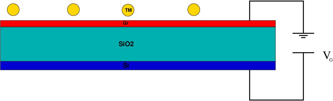
Transport measurements on graphene devices [1] have become standard and can be performed under different doping conditions. Given the location of the Fermi level and the absence of a band gap between the valence and conduction bands in undoped graphene, one can continuously control the level of doping simply by the application of a gate voltage in a geometry where graphene acts as the upper (grounded) electrode of a capacitor. The lower electrode is composed of silicon, whereas the dielectric medium in between is SiO₂. Metal contacts placed on top of the graphene sheet allow for the realisation of transport measurements at different gate voltages, and hence at different levels of doping, with great flexibility. The system has an overall thickness of $b\approx 300$ nm (see figure 1).

The measurement of the transport properties using such devices can be used to determine the influence of different physical effects on both the AC and DC conductivities. One can investigate the influence of electron-electron interactions, of impurities, or of the presence of elastic ripples in the graphene sheet on the transport properties of this semi-metal [3].

It well known that undoped graphene, when analysed from the point of view of a self-consistent theory or the renormalisation group, presents a finite conductivity with an universal value of $4e^{2}/(\pi h)$ [9, 10, 11, 14, 12, 13, 15, 16, 17, 18], regardless of the scattering mechanism that limits conductivity in graphene. The experimental measurements[19, 20] point to a somewhat higher value for this quantity, equal to $4e^{2}/h$. This latter value is also obtained in studies of numerical diagonalisation of graphene’s tight-binding Hamiltonian with add-atoms acting as the source of disorder[21, 22]. In the case of doped graphene, the behaviour of the conductivity markedly depends on the scattering mechanism that limits such quantity. It is therefore essential to clarify the nature of such a mechanism. The research community has held two opposing views, namely charged (Coulomb) or short-range scatterers [23], but recent experiments [24] seem to show the latter mechanism as the prevailing one, even if it is agreed that charged scatterers also play a role [25].

In this paper, we will consider the contribution to the conductivity of one particular type of short-range disorder, namely that induced by the deposition of transition metal (TM) atoms in graphene [26]. This type of disorder is always present on devices such as those depicted in figure 1, due to the diffusion of metallic atoms from the contacts into the graphene sheet. The adsorption of graphene on TM surfaces has been extensively studied, both experimentally [27, 28, 29, 30], as well as theoretically [31, 32, 33, 34, 35, 36]. In TM surfaces for which the adsorption process (physisorption) preserves the conical nature of the graphene bands close to the Dirac point (Al, Ag, Cu, Au, Pt), the authors of [35, 36] have shown that the levels of electron or hole doping of graphene that they have found in their DFT studies can be explained by the relative value of the bulk work-functions of graphene and of that of the transition metal to which graphene is adsorbed. However, in order to explain the electron-doping of graphene in cases where its work-function is lower than that of the transition metal (Ag, Cu), the authors invoked the existence of a chemical interaction between graphene and the underlying metal substrate, which plays a significant role in the formation of surface dipoles[37, 38, 39, 40, 41, 42]. The existence of such an interaction was confirmed in the experimental transport studies of [26], performed on a graphene sheet where TM atoms were deposited, which was part of device such as that of figure 1. The authors of this study have found that in the case of low coverage of graphene by Pt, the metal with the highest work function studied theoretically by [35, 36], graphene is also electronically doped by Pt, becoming hole-doped at higher coverages. The authors stated that the high levels of electron-doping that they have found at low coverages were caused by an increased chemical interaction between graphene and the TM atoms, due to the short-distance (less than $3$ A) between the two species (this distance is equal to $3.3$ A in the full coverage regime). Furthermore, the AFM pictures obtained seem to show that the transition metal atoms aggregate in clusters at low coverage (see also [43]). It is nevertheless unclear whether the proximity between the clusters and graphene is sufficient to justify the level of doping of graphene.

The purpose of this paper is threefold. Firstly, we wish to introduce a framework that allow us to discuss the problem of charge doping of graphene by transition-metal clusters with generality from a thermodynamic point of view. This framework will be of a phenomenological nature and it will involve some simplifying assumptions, but it will already contain the main ingredients that will need to be considered in a more fundamental approach. Secondly, the same type of phenomenological analysis will be extended to the problem of electronic scattering in graphene caused by the presence of the said clusters. We will show, following [44] that, despite the charged nature of the clusters, the scattering potential that they create is of a short-ranged nature (see also [23]). The domain of validity of the semi-classical approximation of independent clusters that we are using is also discussed. Thirdly, these two elements of the theory will be used to interpret the above experiments from a quantitative point of view. This application of the theory will also serve to illustrate its overall limitations and we will provide physical arguments that show why more elaborate approaches are needed.

The structure of this paper is as follows: in section II, we will discuss the doping of graphene by metal clusters in a capacitor device based on a phenomenological model that treats each cluster as a perfectly metallic object kept at a constant potential dependent on the amount of charge in the cluster. The minimisation of the internal energy of the system at $T=0$, subjected to overall charge conservation, will allows us to obtain the equilibrium conditions that determine the level of doping of the graphene sheet. One can show, for equally charged clusters, that the level of doping can be written in terms of the bulk work-functions of the different components of the system, of the gate voltage applied to the device, and of a parameter that characterises the effective chemical interaction between the graphene sheet and each individual cluster. The numerical value of this parameter is determined by two different contributions: the first contribution is due to the induced surface dipole of graphene and of the metallic clusters caused by the presence of the other components of the system; the second contribution is the correction to the Fermi energy of a cluster due to its finite size. Specialising to the case of spherical clusters, we can estimate the magnitude of the chemical interaction using the measured values by[26] of the gate voltage that is necessary to apply to Pt and Ti-covered[45] graphene samples to bring graphene to an uncharged state, where the conductivity is a minimum. These values are dependent on the concentration of metallic atoms per unit cell as well as on which metallic element is deposited on graphene. In section III, we will consider the form of the scattering potential created by a spherical cluster, following the model of [44] and its contribution to the resistivity of the sample, within the First Born Approximation (FBA) and we will compare our results with the transport measurements of[26], performed on Pt-covered graphene samples at low coverage. We will also show why the theory presented is not adequate to explain the measurements performed at higher coverages, both for Pt and Ti-covered samples. We will determine, using the above model, the linear dimension of the region in graphene where the charge donated by the cluster to this material is contained and show that, except for the lowest coverages considered in the experiments of[26], this quantity is comparable to the average distance between clusters, even for heavily-doped graphene. In section IV, we will present our conclusions. In appendix A, we will derive an expression for the cluster’s ionisation potential that will be used in the main text, based on the same thermodynamic arguments that were used in section II. Finally, in appendix B, we will derive, using the method of images, the electrostatic contribution to the ionisation potential of a single spherical cluster, a result that will be shown to be in agreement with that of appendix A. This derivation will also allow us to obtain the capacitance of the system composed of the metallic cluster and of the graphene plane, as well as the electrostatic potential due to a charged spherical cluster close to a grounded plane, a quantity that enters in the calculations performed in section III.

At $T=0$, the internal energy of a composite system of $k$ conductors can be written[46, 47], assuming that the electrons and the (immobile) ions of the different species interact with each other via the bare Coulomb interaction (i.e. one is including the contribution of the low lying electronic orbitals explicitly in the energy), as

where the functional $G(N_{1},\cdots,N_{k})$ includes the kinetic, exchange and correlation energies of the electrons and where the second term includes the effect of the ion potential on the electrons and the Hartree energy of these electrons, with $\rho^{P}_{i}(\mbox{${\boldsymbol{r}}$})=\rho^{e}_{i}(\mbox{${\boldsymbol{r}}$})-\rho^{ions}_{i}(\mbox{${\boldsymbol{r}}$})$ being the plasma charge density. The indices $i,j$ run over $1,\ldots,k$. One can write $\rho^{P}_{i}(\mbox{${\boldsymbol{r}}$})=\rho^{n}_{i}(\mbox{${\boldsymbol{r}}$})+\delta\rho_{i}(\mbox{${\boldsymbol{r}}$})$, where $\rho^{n}_{i}(\mbox{${\boldsymbol{r}}$})$ is the charge density in the neutral ground state of each conductor and $\delta\rho_{i}(\mbox{${\boldsymbol{r}}$})$ is the excess charge density of that conductor due to charge exchange with the others. In particular, $\int_{V_{i}}\,d^{d}r\,\delta\rho_{i}(\mbox{${\boldsymbol{r}}$})=Q_{i}$, the total unbalanced charged contained in conductor $i$. Using this decomposition, one can write the ground-state energy, up to a constant term, as

where ${\cal V}_{i}^{n}(\mbox{${\boldsymbol{r}}$})$ is the potential on conductor $i$ due to itself and the other conductors, each in a neutral state. In a classical approximation, $\delta\rho_{i}(\mbox{${\boldsymbol{r}}$})$ will be non-zero only close to the surface of the conductors, and we can write the above expression in a capacitor approximation:

where $C_{ij}^{-1}$ is the inverse cross-capacitance between conductors $i$ and $j$ and $D_{i}=\overline{{\cal V}_{i}^{n}(\mbox{${\boldsymbol{r}}$})}$ is the surface dipole of conductor $i$[41], which is the average value of the electrostatic potential within that conductor. Note that the surface dipole of a conductor is computed with the remaining conductors present, but in a neutral state. Thus, one expects that such surface dipoles will depend both on the geometry of each conductor and also on the presence of the other conductors if the distances between them are on the atomic scale.

As stated above, the experiments of reference [26] were performed on a devices similar to that depicted in figure 1, with the transition metal atoms deposited by molecular beam epitaxy (MBE) on the graphene sheet at different coverages $c_{S}=N_{am}/n_{u}$ of metallic atoms per unit cell of graphene, where $N_{am}$ is the total number of deposited metallic atoms and $n_{u}$ is the number of graphene’s unit cells. In order to model such a device, we will assume that the atoms aggregate in $N_{c}$ identical clusters, which are randomly distributed above the area $A_{g}=n_{u}A_{c}$ of the graphene sheet, where $A_{c}$ is the area of the graphene unit cell. We also assume that these clusters are all equally charged. The graphene sheet is kept at zero potential. At a distance $b\approx 300$ nm below it, one places a Si layer, with the space in between filled with SiO₂, a medium of permittivity $\epsilon=3.9\,\epsilon_{0}$. The graphene sheet and the Si layer are connected to a battery such that a constant gate-voltage $V_{G}$ is kept between them (’plane-capacitor model’, see figure 2). A single cluster-graphene subsystem is assumed to possess a joint capacitance $C_{S}$ (which is computed for spherical clusters in appendix B). The capacitance of the graphene/SiO₂/Si device is given by $C_{Si}=\epsilon A_{g}/b$. We assume that the cross-capacitance effects between different clusters are only due to the presence of the grounded graphene plane, an assumption that is correct for small $c_{S}$[48].

With such assumptions, the internal energy (3) can be written for this system, as

We have written the charge $Q_{i}$ of a given component $i$ as $Q_{i}=-\,e(N_{i}-N_{i}^{0})$, where $N_{S}$, $N_{g}$ and $N_{Si}$ are, respectively, the number of electrons in a cluster (all clusters are equally charged), in graphene and in the Si layer in the equilibrium state in which these materials are in contact and exchange charge, and $N_{S}^{0}$, $N_{g}^{0}$ and $N_{Si}^{0}$ are the same quantities in the uncharged state of these materials. Also, $D_{S}$, $D_{g}$ and $D_{Si}$ are the surface dipoles of each substance.

The conditions of thermodynamic equilibrium are obtained through the minimisation of (4) subjected to the constraints that the overall charge of the system is zero and that the potential difference between the two electrodes of the battery is equal to $V_{G}$. The minimisation condition is thus given by

since the charge transferred between the electrodes of the battery is $dq=-e\,dN_{Si}$, and where $\mu$ is the chemical potential of the system. One obtains from (5) the following equilibrium conditions

where $\overline{\mu}_{S}=\frac{\partial G}{\partial N_{j}}\mid_{N_{j}=N_{S}}$, with $N_{j}$ being the number of charges in cluster $j$, $\overline{\mu}_{g}=\frac{\partial G}{\partial N_{g}}$, $\overline{\mu}_{Si}=\frac{\partial G}{\partial N_{Si}}$, are the chemical potentials of the different components of the system in the absence of a dipole layer. These quantities are also called the internal contribution of a metal to its work-function[37]. Note that $\mu=\overline{\mu}_{g}-eD_{g}$, i.e. the chemical potential of the system is equal to the (full) chemical potential of the subsystem kept at zero voltage.

The two equilibrium conditions (6,7) are not sufficient to determine the level of doping of the constituents of the system. These equations have to be supplemented with the neutrality condition for the overall system. One can write this condition as

with $\Delta N_{S}=N_{S}-N_{S}^{0}$, $\Delta N_{g}=N_{g}-N_{g}^{0}$ and $\Delta N_{Si}=N_{Si}-N_{Si}^{0}$. The quantities that appear in (8) are related to the variations of the carrier density of the cluster, of graphene, and of the Si layer, by $\Delta N_{S}={\cal V}_{S}\,\delta n_{S}$, $\Delta N_{g}=A_{g}\,\delta n_{g}$ and $\Delta N_{Si}=A_{g}\,\delta n_{Si}$, where ${\cal V}_{S}$ is the volume of the cluster. The number of clusters is given by $N_{c}=N_{am}/n_{amc}$, where $n_{amc}$ is the number of metal atoms per cluster, which is equal to $n_{amc}=z_{S}{\cal V}_{S}/v_{S}$, with $v_{S}$ being the volume of the metallic unit cell and $z_{S}$ being the number of atoms in the unit cell ($z_{S}=1$ for Pt, $z_{S}=2$ for Ti). Expressing $N_{am}$ in terms of $c_{S}$, which was introduced at the beginning of this section, one obtains for $N_{c}$

where we have expressed $n_{u}$ as the ratio between the area of the graphene sheet and the unit cell area. Substituting this formula in equation (8) and expressing $\Delta N_{S}$, $\Delta N_{g}$ and $\Delta N_{Si}$ in terms of the variations of the charge density of each media, one obtains

The equations (6,7), when written in terms of the variations of density $\delta n_{S}$ and $\delta n_{Si}$, become

These two equations, which impose the equality of the so-called electro-chemical potentials[49] between a metallic cluster and the graphene sheet, and between the graphene sheet and the Si layer, when supplemented by (10), are sufficient to determine the level of doping of graphene. However, we still need to relate the chemical potential $\overline{\mu}_{S}$ to $\delta n_{S}$, $\overline{\mu}_{g}$ to $\delta n_{g}$ and $\overline{\mu}_{Si}$ to $\delta n_{Si}$, in other words, we need the equation of state for the different components of the system. One writes $\Delta\varepsilon_{F}^{S}=\overline{\mu}_{S}-\varepsilon_{F}^{S}$ for the Fermi energy variation of the cluster, $\Delta\varepsilon_{F}^{g}=\overline{\mu}_{g}-\varepsilon_{F}^{g}$ for the Fermi energy variation of graphene and $\Delta\varepsilon_{F}^{Si}=\overline{\mu}_{Si}-\varepsilon_{F}^{Si}$ for the Fermi energy variation of the Si layer, measured with respect to the uncharged ground state of each of these constituents. In the case of the clusters or of the Si layer, one has $\delta n_{S}\approx\rho_{S}(\varepsilon_{F}^{S})\,\Delta\varepsilon_{F}^{S}$ and $\delta n_{Si}\approx\rho_{Si}(\varepsilon_{F}^{Si})\,\Delta\varepsilon_{F}^{Si}$ since the density of states $\rho(\varepsilon_{F})$ is approximately constant for these materials at the Fermi level. Substituting these definitions in (11) and (12) and taking into account that the bulk work functions of the transition metal, of graphene, and of Si, are given by $W_{B}=eD_{B}-\varepsilon_{F}^{B}$, $W_{g}^{0}=eD_{g}^{0}-\varepsilon_{F}^{g}$ and $W_{Si}^{0}=eD_{Si}^{0}-\varepsilon_{F}^{Si}$[39], one obtains

where $\zeta_{S}=\varepsilon_{F}^{S}-\varepsilon_{F}^{B}$ is the difference between the Fermi energy of the TM cluster and the Fermi energy of the bulk transition-metal and $\Delta D_{S}=D_{S}-D_{B}$, $\Delta D_{g}=D_{g}-D_{g}^{0}$ and $\Delta D_{Si}=D_{Si}-D_{Si}^{0}$ are the induced surface dipoles on each component of the system due to finite size effects and to the presence of the other components. One can estimate $\rho_{Si}(\varepsilon_{F}^{Si})\approx\frac{m^{*}_{Si}}{\pi\hbar^{2}}$, the result for a free two-dimensional electron gas, where $m^{*}_{Si}\approx m_{e}$ is the electron’s effective mass in Si. With $b\approx 300$ nm, one has $\rho_{Si}(\varepsilon_{F}^{Si})\gg\epsilon/(e^{2}b)$ and one can neglect the first term in the denominator of (14). One can thus write (13,14) as

where $\Delta_{c}=\zeta_{S}+e(\Delta D_{g}-\Delta D_{S})$ represents a correction to the doping of the clusters due to their finite size and to the induced surface dipoles, and $V_{0}=(W_{Si}^{0}-W_{g}^{0})/e+\Delta D_{Si}-\Delta D_{g}$. The quantity $\Delta_{c}$ can be interpreted as giving the overall magnitude of the effective chemical interaction between the clusters and the graphene sheet.

The density of states $\rho_{g}(\epsilon)$ of graphene is zero at the Dirac point and one needs to consider its full functional form in that neighbourhood. It is approximately given by[25]

where $t=2.7$ eV is the first-nearest neighbour hopping matrix element in graphene. Note that the presence of impurities in graphene, either intrinsic or the deposited TM atoms themselves, will modify the density of states given in (17) for high enough impurity concentrations[16]. Integrating $\rho_{g}(\varepsilon)$ between the lower band limit $\varepsilon_{F}^{g}-\sqrt{\sqrt{3}\pi}t$ and the Fermi energy $\varepsilon_{F}^{g}$ [15] yields a result of two electrons per unitary cell.

Integrating $\rho_{g}(\varepsilon)$ between $\varepsilon_{F}^{g}$ and $\mu_{g}$, one obtains for $\delta n_{g}$ the result

with the plus sign if $\Delta\varepsilon_{F}^{g}>0$ and the minus sign otherwise.

Substituting equations (15), (16) and (18) in (10), we finally obtain a second-degree equation for $\Delta\varepsilon_{F}^{g}$

with the plus sign if $\Delta\varepsilon_{F}^{g}>0$ and negative sign otherwise, and where

If we take the positive sign in equation (19) then a positive solution exists if $\Omega>0$. Conversely, if we take the negative sign in this equation, a negative solution exists if $\Omega<0$. One can thus write for $\Delta\varepsilon_{F}^{g}$, the solution [50]

One can see from equation (22) that for a given concentration $c_{S}$, one can, through the application of a gate-voltage $V_{D}$ such that $\Omega=0$, bring the graphene sheet to its uncharged state, as $\Delta\varepsilon_{F}^{g}=0$. The gate voltage $V_{D}$ can be determined from transport measurements on Pt or Ti-covered graphene[26], since the conductivity will display the minimum characteristic of the Dirac point for that applied voltage. Likewise, the gate voltage $V_{0}$ can be determined from the same measurements performed on the uncovered graphene samples, since it follows from equation (22) that for $c_{S}=0$, $\Delta\varepsilon_{F}^{g}=0$ at $V_{G}=V_{0}$. Thus, the conductivity will also display the characteristic minimum at this applied voltage. Therefore, one can extract $\Delta_{c}$ from experiment. It is given by

The density of states at the Fermi level of bulk Pt or bulk Ti can be extracted from specific heat measurements[51, 52], through $\rho(\varepsilon_{F}^{B})=3\gamma/(\pi k_{B})^{2}$, using the general result from Landau’s Fermi liquid theory, where $\gamma$ is the linear coefficient for the dependence of the electronic specific heat $c_{V}$ on the temperature. Finite size corrections to the bulk density of states may be estimated for a spherical cluster, using the results for a free-electron gas [53], as $\rho_{S}(\varepsilon_{F}^{S})=\rho(\varepsilon_{F}^{B})-3m^{*}/(8\pi\hbar^{2}R)$, where $m^{*}_{Pt}\approx 2m_{e}$[54], $m^{*}_{Ti}\approx 3.15m_{e}$[52] is the electron’s effective mass in platinum or titanium and $R$ is the radius of the cluster. Also, for a spherical cluster, ${\cal V}_{S}=4\pi R^{3}/3$ and $C_{S}$ can be written as a power series on a parameter dependent on the cluster radius and on the distance $L$ of its centre to the graphene sheet (see appendix B). We take $W_{g}^{0}=4.5$ eV as in [26], $W_{Pt}^{0}=5.64$ eV and $W_{Ti}^{0}=4.33$ eV for polycrystalline platinum and polycrystalline titanium, and $W_{Si}^{0}=4.6$ eV[55]. We note that the model as defined contains two unknown parameters, namely $R$ and $L$.

Using these results, as well as the values of $c_{S}$, $V_{0}$ and $V_{D}$ measured by [26] (raw data is a courtesy of Kawakami’s group) and taking the radius of the cluster to be $0.6$ nm for Pt[56] and $0.188$ nm for Ti [57] and the distance from the centre of the cluster to the plane equal to $0.85$ nm for Pt and $0.44$ nm for Ti, one obtains for $\Delta_{c}$ the results given in tables 1, 2 and 3. Note that one does not dispose of direct information (e.g. from AFM measurements) regarding the values of $R$ and $L$. The values indicated above were chosen such as to provide agreement between the values of $\Delta_{c}$ and $\Delta_{c}^{est}$ in tables 1, 2 and 3, as well as between the theoretical and experimental asymptotic values for the contribution to the resistivity coming from the presence of the clusters[58] (see section III). We have considered here and below the measurements made with samples Pt-1, Pt-3 and Ti-1 (in the notation of [26]), since these samples, when uncovered, presented the smallest values of $V_{0}$ measured, indicating a low level of intrinsic disorder.

One can estimate the correction to the Fermi energy, due to the cluster’s finite radius, from the free-electron gas result, as $\zeta_{S}\approx\frac{3\pi^{2}\hbar^{4}}{8(m^{*})^{2}R}\,\cdot\rho(\varepsilon_{F}^{B})$. Using the result quoted in the references [35, 36] for the induced dipole $e\,(\Delta D_{g}-\Delta D_{S})\approx 0.9$ eV[59], one obtains for $\Delta_{c}^{est}$ the results presented in tables 1, 2 and 3 for Pt and Ti, respectively. Thus, it is seen that the larger value of the chemical interaction $\Delta_{c}$ with respect to the case studied in[35, 36] (particularly in platinum that has a larger DOS at the Fermi level) is due to a large shift of the Fermi energy of the clusters with respect to that of the bulk TM metal, caused by their finite radius.

For a small cluster, the concept of work-function is ill-defined[60], as this quantity depends on the cluster’s charge. One then speaks, respectively, of the cluster’s ionisation potential if one is withdrawing an electron from a cluster at equilibrium, or of the cluster’s electron affinity, if the electron is withdrawn from a negatively over-charged cluster. In appendix A, we compute the ionisation potential of a cluster based on a thermodynamic argument. We obtain from (46) the result

for the ionisation potential of the metallic cluster, where $\Delta\varepsilon_{F}^{g}$ is given by (22). Substituting in (24) the parameters as computed in table 1, we have plotted in Figures 3, 4 and 5 the result (24) as function of the applied voltage, for the different coverages $c_{S}$ considered in [26], for their Pt-1, Pt-3 and Ti-1 samples[61]. In these plots, we have ignored the (unknown) constant $e\Delta D_{g}$[62]. Nevertheless, such constant shift should be obtainable from a plot of the experimental ionisation potential, and so provide an estimate of $e\Delta D_{g}$.

It is also shown in appendix A that the electron affinity $A_{S}$ of a metallic cluster is given by $A_{S}=I_{S}-e^{2}/C_{S}$, with $W_{g}=\frac{1}{2}(I_{S}+A_{S})$. Thus, $A_{S}<W_{g}<I_{S}$. Since the transfer of an electron from the cluster to graphene would cost an energy $I_{S}-W_{g}>0$ and, conversely, the transfer of an electron from graphene to the cluster would cost the same energy $W_{g}-A_{S}>0$, one sees that the equilibrium state defined by equations (10) to (12) is indeed a stable one. The theory exposed in this section constitutes the main result of this paper.

In the previous section, we have computed the level of doping of a graphene sheet due to the presence of metallic clusters. We have also computed the ionisation potential of a single cluster. These properties are equilibrium properties. However, the experiments of [26] measured the dependence of the conductivity of graphene on the doping induced by the metallic clusters and by the applied gate voltage. In order to describe such dependence, one needs to determine the scattering potential on individual carriers due to the presence of the clusters. We will determine such a potential for spherical clusters, in an electrostatic approximation, which allows for the use of the method of images. Note that in such approximation, the graphene sheet is an equipotential surface. Therefore, the Coulomb interaction due to the surface charge distribution of the clusters is perfectly screened by the surface charge distribution that it is generated on the graphene sheet. However, such induced charge distribution is spatially varying and it will thus correspond to a local variation of the Fermi level of graphene [44]. Such variation will enter in the Dirac equation that describes the low-energy properties of graphene as a scattering potential and will give rise to a variation of the conductivity. Note that the local variation of the Fermi energy due to a cluster is not a parameter of the model as in [23], but depends on the level of doping of graphene.

The clusters, of radius $R$, are placed at a distance $L>R$ above the graphene sheet. Each cluster possesses a charge $Q_{S}=-e\Delta N_{S}=-\frac{4}{3}\pi R^{3}e\,\delta n_{S}$. We place the origin of the coordinate axis aligned with the centre of the spheres, such that the graphene sheet is located at $z=-L$. In the subspace $z\geq-L$, the electrostatic potential can be approximately described by the superposition

of the potentials due to the individual clusters, located at $\mbox{${\boldsymbol{r}}$}_{i}=(x_{i},y_{i},0)$.

In appendix B, we will show how $v(\mbox{${\boldsymbol{r}}$})$ can be written in terms of a series of image charges, located in the cluster, and their images, located below the graphene plane. These charges depend on $Q_{S}$, $R$ and $L$ through a recursion relation.The displacement field in the subspace $z\geq-L$ is given by $\mbox{${\boldsymbol{D}}$}=-\epsilon_{0}\,\nabla V(\mbox{${\boldsymbol{r}}$})$, whereas it is equal to $\mbox{${\boldsymbol{D}}$}=-e\,\delta n_{Si}\,\mbox{${\boldsymbol{e}}$}_{z}$ in the space between the graphene sheet and the Si layer. The discontinuity of its normal component at $z=-L$ determines the local density of charge $\sigma_{g}(x,y)$ in the graphene sheet. In terms of the density of carriers $\delta n_{g}(x,y)=-\sigma_{g}(x,y)/e$, one has

where the derivative with respect to $z$ is evaluated at the location of the graphene plane, $z=-L$. The spatial average of $\delta n_{g}(x,y)$ is given by equation (10). Averaging equation (26), we thus obtain $\left.\overline{\frac{\partial V(\mbox{\bf\scriptsize r})}{\partial z}}\right|_{-L}=-\frac{ec_{S}v_{S}}{\epsilon_{0}z_{S}A_{c}}\,\delta n_{S}$. Furthermore, one can write equation (26) as

The precise form of the local density of carriers depends on the location of the metallic clusters. However, assuming that one can treat clusters as independent entities, one has that in the neighbourhood of a given cluster, located at the origin of the coordinates, one can approximate (27) by

where $v(\mbox{${\boldsymbol{r}}$})$ is given by (59). Using the previous results, one can also estimate that

where $N_{c}$ is the number of clusters. Since such a number is supposed to be very large, this term is negligible and one has that

Substituting equations (59) and (60) for $v(\mbox{${\boldsymbol{r}}$})$ in (30) and expressing $Q_{S}$ in terms of $\delta n_{S}$ as above, one obtains the following series for $\delta n_{g}(r)$[63]

where $\lambda=\frac{1}{R}\,(L-\sqrt{L^{2}-R^{2}})$ and where $g(\lambda,1)$ is given by (54).

The local variation of the carrier density $\delta n_{g}(r)$ in graphene is related to the local variation of the Fermi energy $\Delta\varepsilon_{F}^{g}(r)$ through equation (18). Assuming that one is far from the neutrality point of graphene and that $\Delta\varepsilon_{F}^{g}(r)$ and $\Delta\varepsilon_{F}^{g}$ have the same sign, one has that the difference $U(r)=\Delta\varepsilon_{F}^{g}-\Delta\varepsilon_{F}^{g}(r)$ is given approximately by

where $\Delta\varepsilon_{F}^{g}$ is given by (22) and $\delta n_{S}$ is given by (15). The function $U(r)$ is the electron scattering potential due to a single cluster and depends, in this approximation, on the cluster carrier density $\delta n_{S}$ and also on the level of doping of graphene itself (through its dependence on $\mid\Delta\varepsilon_{F}^{g}\mid$). Note that $U(r)$ is attractive if $\delta n_{S}<0$ (the cluster is doped with holes, as seen in experiment), as one would expect. The plot of $U(r)$ is given, for different values of the gate voltage $V_{G}$, in figure 6.

We can also compute from (31), for later use, the size of the region in graphene that contains a charge $-Q_{S}$ of equal magnitude to that of an individual clusters, in the case in which graphene is electron-doped (i.e. for $V>V_{D}$). We integrate equation (31) within the disk $r<R_{S}$, the region whose size we wish to calculate. We obtain after some cancellations, the following equation for $R_{S}$

This quantity should be compared with the average distance $R_{c}$ between clusters, that can be simply defined through the relation $\pi R_{c}^{2}=A_{g}/N_{c}=\frac{4\pi R^{3}A_{c}z_{S}}{3c_{S}v_{S}}$, i.e. in terms of the average area per cluster. If one defines the ratio $\xi=R_{S}/R_{c}$ between these two quantities, one has, noting that the second fraction in the infinite sum of (33) can be simply approximated by $R_{S}^{-1}$ if $R_{S}\gg L$, that $\xi$ is approximately given by

where the first term is a constant for fixed $L$ and $R$. The validity of the independent cluster approximation, assumed above when passing from (27) to (28), depends on the condition $\xi<1$[64] being fulfilled.

The contribution of the metallic clusters to the resistivity of the sample of graphene can be easily computed within the FBA, once the scattering potential is known. Within the semi-classical theory[4] based on the Boltzmann equation, the contribution of the clusters to the conductivity of the sample is given by

where $v_{F}=\frac{\sqrt{\sqrt{3}A_{c}/2}\,t}{\hbar}$ is the Fermi velocity in graphene, $k_{F}=\frac{\mid\Delta\varepsilon_{F}^{g}\mid}{\hbar v_{F}}$ is the momentum of a quasi-particle at the Fermi surface of doped graphene, measured with respect to the Dirac point, and $\tau_{cl}(k_{F})$ is the transport lifetime of a quasi-particle at the Fermi surface, due to the scattering with the metallic clusters. The expression above already accounts for the double spin and valley degeneracy (existence of two independent Dirac points). Equation (35) is known to apply as long as $k_{F}l_{e}\gg 1$, where $l_{e}$ is the electron mean-free path. This condition holds in the diffusive regime where graphene is highly-doped (i.e. far away from the Dirac point) and for low-impurity concentration. The inverse of $\tau_{cl}(k_{F})$ can be computed in the FBA, by the application of Fermi’s Golden-Rule

where $N_{c}$ is as above the number of clusters, i.e. the number of scattering centres, $\mid\!\mbox{${\boldsymbol{k}}$}\!\mid\,=k_{F}$, $\varepsilon_{\mbox{\bf\scriptsize k}}=\hbar v_{F}\mid\!\mbox{${\boldsymbol{k}}$}\!\mid$, $\varepsilon_{\mbox{\bf\scriptsize k}^{\prime}}=\hbar v_{F}\mid\!\mbox{${\boldsymbol{k}}$}^{\prime}\!\mid$, $\hat{\mbox{${\boldsymbol{k}}$}}$, $\hat{\mbox{${\boldsymbol{k}}$}}^{\prime}$ are the unit vectors in the direction of ${\boldsymbol{k}}$ and $\mbox{${\boldsymbol{k}}$}^{\prime}$ and $U(r)$ is given by (32).

In (36), one needs to take into account the spinorial nature of the wave-functions $\mid\mbox{${\boldsymbol{k}}$}\,\rangle$, $\mid\mbox{${\boldsymbol{k}}$}^{\prime}\,\rangle$. The spinor $u_{\mbox{\bf\scriptsize k}}(\mbox{${\boldsymbol{r}}$})=\langle\,\mbox{${\boldsymbol{r}}$}\,\mbox{$\mid\mbox{${\boldsymbol{k}}$}\,\rangle$}$, which is normalized over the area $A_{g}$ of the sample is given by

where $\tan\theta_{\mbox{\bf\scriptsize k}}=k_{y}/k_{x}$. The $\pm$ signs stand for states with the same momentum and opposite energies relative to the Dirac point. The expression for $u_{\mbox{\bf\scriptsize k}^{\prime}}(\mbox{${\boldsymbol{r}}$})$ is entirely analogous.

Substituting (37) and the analogous expression for $u_{\mbox{\bf\scriptsize k}^{\prime}}(\mbox{${\boldsymbol{r}}$})$ in (36), converting the summation over $\mbox{${\boldsymbol{k}}$}^{\prime}$ into an integral, performing the integral over $k^{\prime}$ using the delta function and expressing $N_{c}/A_{g}=\frac{3c_{S}v_{S}}{4\pi R^{3}z_{S}A_{c}}$, we obtain the following result in terms of an angular integral over the scattering angle $\phi=\theta_{\mbox{\bf\scriptsize k}^{\prime}}-\theta_{\mbox{\bf\scriptsize k}}$,

The expression (38), as it stands, cannot be written in terms of elementary functions. However, the resulting integral is elementary if one can substitute the exponential functions in the infinite sum by $1$, i.e. if their exponents are very small. The largest exponent is the one coming from the term with $n=1$ and is equal to $2k_{F}L\sin(\phi/2)$. Thus, this approximation is valid if $k_{F}L\ll 1$. Since $\delta n_{g}=\pm\frac{k_{F}^{2}}{\pi}$, one can write the above condition as $\mid\!\delta n_{g}\!\mid\ll\frac{1}{\pi L^{2}}$. Taking $L\approx 1$ nm, one obtains from this condition that $\mid\!\delta n_{g}\!\mid\ll 10^{13}-10^{14}\,\mbox{e}/\mbox{cm}^{2}$. This condition is obeyed for all experimentally applied voltages. Thus, substituting the resulting expression for $\tau_{cl}(k_{F})$ in (35), one obtains

References

- [1] K. S. Novoselov, A. K. Geim, S. V. Morozov, D. Jiang, Y. Zhang, S. V. Dubonos, I. V. Grigorieva and A. A. Firsov, Science 306, 666 (2004).
- [2] K. S. Novoselov, D. Jiang, T. Booth, V.V. Khotkevich, S. M. Morozov and A. K. Geim, PNAS 102, 10451 (2005).
- [3] A.H. Castro Neto, F. Guinea, N.M.R. Peres, K.S. Novoselov and A.K. Geim, Rev. Mod. Phys. 81, 109 (2009).
- [4] D. Abergel, V. Apalkov, J. Berashevich, K. Ziegler and T. Chakrabortya, Adv. Phys. 59, 261 (2010).
- [5] L. X. WangZhi and K. Mullen, Nano Lett. 8, 323 (2008).
- [6] P. Blake, P. D. Brimicombe, R. R. Nair, T. J. Booth, D. Jiang, F. Schedin, L. A. Ponomarenko, S. V. Morozov, H. F. Gleeson, E. W. Hill, A. K. Geim and K. S. Novoselov, Nano Lett. 8, 1704 (2008).
- [7] F. Schedin, A. K. Geim, S. V. Morozov, D. Jiang, E. H. Hill, P. Blake and K. S. Novoselov, Nature Materials 6, 652 (2007).
- [8] X. Wang, Y. Ouyang, X. Li, H. Wang, J. Guo and H. Dai, Phys. Rev. Lett. 100, 206803 (2008).
- [9] N. Schon and T. Ando, J. Phys. Soc. Jpn. 67, 2421 (1998).
- [10] Y. Zheng and T. Ando, Phys. Rev. B 65, 245420 (2002).
- [11] P. M. Ostrovsky, I. V. Gornyi and A. D. Mirlin, Phys. Rev. B 74, 235443 (2006).
- [12] N. M. R. Peres, F. Guinea, and A. H. Castro Neto, Phys. Rev. B 73, 125411 (2006).
- [13] T. Stauber, N. M. R. Peres, and A. H. Castro Neto, Phys. Rev. B 78, 085418 (2008).
- [14] M. Katsnelson, Eur. Phys. J. B 51, 157 (2006).
- [15] B. Dóra, K. Ziegler and P. Thalmeier, Phys. Rev. B 77, 115422 (2008).
- [16] N. Leconte, J. Moser, P. Ordejón, H. Tao, A. Lherbier, A. Bachtold, F. Alsina, C. M. Sotomayor Torres, J. C. Charlier and S. Roche, ACS Nano 4, 4033 (2010).
- [17] A. Lherbier, B. Biel, Y. M. Niquet and S. Roche, Phys. Rev. Lett. 100, 036803 (2008).
- [18] A. Lherbier, S. M. -M. Dubois, X. Declerck, S. Roche, Y. M. Niquet and J. C. Charlier, Phys. Rev. Lett. 106, 046803 (2011).
- [19] A. K. Geim and K. S. Novoselov, Nature Mater. 6, 183 (2007).
- [20] Y. W. Tan, Y. Zhang, K. Bolotin, Y. Zhao, S. Adam, E. H. Hwang, S. Das Sarma, H. L. Stormer and P. Kim, Phys. Rev. Lett. 99, 246803 (2007).
- [21] A. Lherbier, X. Blase, Y. M. Niquet, F. Triozon and S. Roche, Phys. Rev. Lett. 101, 036808 (2008).
- [22] A. Ferreira, J. Viana-Gomes, J. Nilsson, E. R. Mucciolo, N. M. R. Peres and A. H. Castro Neto, Phys. Rev. B 83, 165402 (2011).
- [23] M. I. Katsnelson and F. Guinea and A. K. Geim, Phys. Rev. B 79, 195426 (2009).
- [24] L. A. Ponomarenko, R. Yang, T. M. Mohiuddin, M. I. Katsnelson, K. S. Novoselov, S. V. Morozov, A. A. Zhukov, F. Schedin, E. W. Hill and A. K. Geim, Phys. Rev. Lett. 102, 206603 (2009).
- [25] N. M. R. Peres, Rev. Mod. Phys. 82, 2673 (2010).
- [26] K. Pi, K. M. McCreary, W. Bao, Wei Han, Y. F. Chiang, Yan Li, S.-W. Tsai, C. N. Lau and R. K. Kawakami, Phys. Rev. B 80, 075406 (2009).
- [27] S. Marchini, S. Günther, and J. Wintterlin, Phys. Rev. B 76, 075429 (2007).
- [28] A. L. Vázquez de Parga, F. Calleja, B. Borca, M. C. G. Passeggi, J. J. Hinarejos, F. Guinea, and R. Miranda, Phys. Rev. Lett. 100, 056807 (2008).
- [29] P. W. Sutter, J. I. Flege, and E. A. Sutter, Nature Mater. 7, 406 (2008).
- [30] A. B. Preobrajenski, M. L. Ng, A. S. Vinogradov and N. Martensson, Phys. Rev. B 78, 073401 (2008).
- [31] K. T. Chan, J. B. Neaton and M. L. Cohen, Phys. Rev B 77, 235430 (2008).
- [32] Y. Mao, J. Yuan and J. Zhang, J. Phys. Cond. Mat. 20, 115209 (2008).
- [33] B. Wang, M. L. Bocquet, S. Marchini, S. Günther and J. Wintterlin, Phys. Chem. Chem. Phys. 10, 3530 (2008).
- [34] D. Jiang, M. Du and S. Dai1, J. Chem. Phys. 130, 074705 (2009).
- [35] G. Giovannetti, P. A. Khomyakov, G. Brocks, V. M. Karpan, J. van den Brink and P. J. Kelly, Phys. Rev. Lett. 101, 026803 (2008).
- [36] P. A. Khomyakov, G. Giovannetti, P. C. Rusu, G. Brocks, J. van den Brink and P. J. Kelly, Phys. Rev. B 79, 195425 (2009).
- [37] F. Seitz, The modern theory of solids, McGraw-Hill, New York (1940).
- [38] C. Herring and M. H. Nichols, Rev. Mod. Phys. 21, 185 (1949).
- [39] N. D. Lang and W. Kohn, Phys. Rev. B 3, 1215 (1971).
- [40] V. Heine and C. H. Hodges, J. Phys. C 5, 225 (1972).
- [41] N. D. Lang and W. Kohn, Phys. Rev. B 8, 6010 (1973).
- [42] J. L. F. Da Silva, C. Stampfl and M. Scheffler, Phys. Rev. Lett. 90, 066104 (2003).
- [43] K. M. McCreary, K. Pi, A. G. Swartz, W. Han, W. Bao, C. N. Lau, F. Guinea, M. I. Katsnelson and R. K. Kawakami, Phys. Rev. B 81, 115453 (2010).
- [44] M. M. Fogler, D. S. Novikov and B. I. Shklovskii, Phys. Rev. B 76, 233402 (2007).
- [45] According to the studies of [31, 36], Ti is chemically adsorbed in graphene and does not preserve the Dirac point in the newly computed band structure. However, since the maximum concentration of Ti studied by [26] is below , one does not expect that in this case the band structure will be significantly changed with respect to pristine graphene.
- [46] P. Hohenberg and W. Kohn, Phys. Rev. 136, B864 (1964).
- [47] W. Kohn and L. J. Sham, Phys. Rev.140, A1133 (1965).
- [48] The assumption that the cross-capacitance between two clusters and is solely due to the presence of the graphene plane can be expressed mathematically as , where , and are, respectively, the inverse cross capacitance of two clusters, the inverse cross capacitance between a cluster and the graphene plane and the inverse self-capacitance of graphene. Writing the joint capacitance of two clusters as , since , and using the equation above, we see that this expression is equivalent to the equality , where is the joint capacitance of a cluster and the graphene plane. Note that in the derivation of (4) the assumption that , i.e. that the cross-capacitance between the clusters and the Si sheet is due to two capacitors in series, is also used.
- [49] O. Madelung, Introduction to solid-state theory, 3rd ed., Springer Verlag, 1996.
- [50] Equation (22) is also valid for a simple capacitor geometry in the absence of deposited metal. In that case, one sees that for the parameters as given in experiments made with capacitor like devices, and hence the doping of graphene is very well described by a simple capacitor law [1], except in the neighbourhood of the Dirac point.
- [51] O. K. Andresen, Phys. Rev. B 2, 883 (1970).
- [52] I. Estermann, S. A. Friedberg and J. E. Goldman, Phys. Rev.87, 582 (1952).
- [53] D. L. Hill and J. A. Wheeler, Phys. Rev. 89, 1102 (1953).
- [54] J. B. Ketterson and L. R: Windmiller, Phys. Rev. B 2, 4813 (1970).
- [55] CRC Handbook of Chemistry and Physics, 90th Edition, Taylor and Francis 2009-2010.
- [56] A spherical cluster of Pt atoms with A contains approximately 60 atoms of platinum.
- [57] A spherical cluster of Ti atoms with A contains only 2 atoms of titanium. It is thus debatable if a continuum theory such as the one presented above is applicable. The relative agreement obtained may be accidental, see [61].
- [58] The experimental results of [26] allow one to place a limit on the minimal distance between the clusters and the graphene sheet, i.e. A. We have therefore chosen A, although the results for are only very weakly dependent on , unlike what happens with .
- [59] The result of references[35, 36] for the induced dipoles was obtained for a system of a single graphene sheet adsorbed on a bulk transition metal and hence does not take into consideration the effect of the finite size of the clusters.
- [60] K.H. Meiwes-Broer, Hyp. Int. 89, 263 (1994).
- [61] The ionisation potential of a Ti cluster computed from (24) is eV. This value is similar to the average ionisation energy of eV of an isolated Ti atom, if we consider the average doping of e/Ti atom, using the first and second ionisation energies of the titanium atom. The relative coincidence of these two values may help explain why one is still able to apply a continuum theory to describe essentially isolated titanium atoms.
- [62] The computed work-function of graphene adsorbed on (111) platinum in [35, 36] is eV with . This is to be compared with the value of the work function at zero gate voltage obtained from (24) for the largest coverage considered above, if we neglect the induced dipole, which is equal to eV. Hence, eV, at large coverages.
- [63] Performing the spatial averaging of the second term of equation (31) over a disc of radius , one obtains, to leading order in , the result given by equation (29) (multiplied by ).
- [64] We are grateful to P. Fulde for having called our attention to the need to estimate the ratio , so as to determine the domain of validity of the independent cluster approximation.
- [65] J. Jeans, The mathematical theory of electricity and magnetism, 5th ed., CUP, 1933.
- [66] In order to achieve faster numerical convergence [65], one should represent .