Quota Complexes, Persistent Homology and the Goldbach Conjecture

In the area of voting theory in political science, monotone yes/no voting systems are studied. If $V$ is a set of voters, then a subset of voters, $C\subset V$ is called a losing coalition if the voters in $C$ are not sufficient to force an initiative to pass. One can form a simplicial complex (see [H] or [Mu] for background on simplicial complexes) $X$ with vertex set $V$ to encode the voting system by declaring $F=[v_{0},\dots,v_{n}]$ to be a face of $X$ if and only if $\{v_{0},\dots,v_{n}\}$ is a losing coalition. The monotone property of the voting system then guarantees that any face of a face in $X$ is also a face in $X$ and so $X$ is indeed a simplicial complex. In voting theory, it is shown that every voting system can be weighted so that it is a quota system. In this paper we study the topological behaviour of various quota complexes as the quota is changed. The issues involved are essentially those involved in Morse theory or persistant homology where the change in topology of a set is studied as a parameter is increased.

For example in [EH] and [Ka], the topology of a finite union of balls of radius $r$ in $\mathbb{R}^{n}$, is studied as a function of $r$ for fixed centers. This is used both in generating random complexes and in studying the persistant shapes/homology of random data sets.

In this paper we first discuss some basic topological properties of quota sets. We then illustrate the theory with examples in arithmetic involving the distribution of primes, squares, cubes and divisors of a fixed number.

In all these cases, the quota complexes encode significant distributional information and our aim is to illustrate some of this.

Let $\mathbb{R}_{+}$ be the set of positive real numbers.

For example, if we have 3 vertices $\{a,b,c\}$ with weights $\{2,3,5\}$ respectively then at quota $q=9$, the corresponding quota complex would be the boundary of a triangle with corners $\{a,b,c\}$. The interior would not be included as the face $[a,b,c]$ has weight $2+3+5=10>9$. If the quota is raised to $11$, this face would be included to give a solid triangle whereas if the quota were lowered to $8$, the edge $[b,c]$ would be excluded from the complex as it has weight $3+5=8$.

In the appendix, it is shown that every finite simplicial complex is isomorphic to a vector-valued quota complex $X[\hat{w}:\hat{q}]$ where the weights and quota can be taken to be vectors with positive integer entries.

In section 2, the basic topology of quota complexes is studied especially scalar-valued quota complexes. One of the key results is (all the relevant topological definitions can be found in that section):

These quota systems are then applied to examples in number theory (for the basic background needed in number theory see for example [A] or [Te]) :

The prime complex is the full simplicial complex with vertex set equal to the set of primes $P=\{2,3,5,7,11,\dots\}$. For a fixed integer $q\geq 3$, $Prime(q)$ is the quota complex on vertex set $P$ and quota $q$ (thus the actual vertex set will be all primes less than $q$ and the faces will be collections of such primes whose sum is less than $q$.)

In section 3 we study this basic prime complex and show

Thus while the $Prime(q)$ complex is defined as a natural quota complex with vertices the set of primes less than $q$ and faces given by collections of such primes whose sum is less than $q$, the topology of the complex $Prime(q)$ is carried by the sums whose sum lies in the shell $[q,q-2)$. Hence one can view the statement above as a topological form of the sieve method important in number theory.

In the section 3 we also include data that shows how $H_{i}(Prime(q))$ varies as a function of $q$ for fixed $i$. The behaviour observed is similar to that found in the study of random simplicial complexes (see [Ka]) and to behaviour observed in the birth-death process in the theory of continuous Markov chains (see [LR]).

In section 5 we study how another topological quantity namely the Euler characteristic of $Prime(q)$ varies as the quota $q$ is changed. We find

where $\mu$ is the Möbius function and $L_{q}$ is a certain characteristic function which converges pointwise to the characteristic function of the square-free integers as $q\to\infty$. In order to clarify the issue, we introduce the LogPrime quota complex which is the simplicial complex on the set of primes as vertices but with the weight of a vertex $p$ being $ln(p)$. We then study how the Euler characteristic of this quota complex changes with quota and obtain:

The substance of this theorem is really due to the work of Titchmarsh (see [Ti]) who gave an equivalent statement to the Riemann Hypothesis based on the rate of growth of Merten’s function. However we include it to point out that the problem also can be cast as a question about quota complexes.

In section 4 we give data for similar complexes encoding the distribution of integer squares and cubes. For example one can let $Square(q)$ be the simplicial complex on vertices the positive integer squares less than $q$ and with the faces consisting of collections of positive integer squares whose sum is less than $q$. Similarly one can define a complex $Cube(q)$ where cubes replace squares.

One then gets similar flavor theorems:

Data describing the growth of $H_{i}$ for these two complexes as a function of $q$ is also presented in that section.

As a final arithmetical application, in section 6 we define for any integer $n\geq 2$, the divisor complex $Div(n)$ whose vertices consist of the proper positive integer divisors of $n$ and whose faces consist of collections of such divisors whose sum is less than $n$. (Hence we are using quota $n$). This complex encodes the distribution of the divisors of $n$, keeping track of which collections of divisors have sums less than $n$ or greater or equal to $n$.

Recall an integer $n\geq 2$ is called deficient if the sum of its proper divisors is less than $n$, perfect if the sum of its proper divisors is equal to $n$, and abundant if the the sum of its proper divisors is greater than $n$. We obtain the following theorem:

The complex $Div(n)$ in the case that $n$ is abundant can be relatively complicated. Data is presented in section 6 which shows an example of an odd number whose complex $Div(n)$ is spherical and of dimension close to $\tau(n)-3$ but not equal. This odd number is “close” to being an odd perfect number in a topological sense; of course the existence of an actual odd perfect number is still open. Even perfect numbers are in bijective correspondence with Mersenne primes and it is an open question whether there are infinitely many of these.

In section 7, a generating function for Euler characteristics of quota complexes is found and a quota-complex formulation of Lehmer’s conjecture is provided among other things.

In the final section, we consider a finite set of independent continuous random variables $X_{1},\dots X_{N}$ with continuous density functions $f_{i}$ with compact support in $[m,\infty)$ where $m>0$. We examine the random quota complex associated to these random variables with fixed minimal weight $X_{0}=m$ and quota $q>m>0$. We derive various formulas for the expected topology of this complex (see the section for the relevant definitions and [B] for basic background.)

We then give an example where the final equality in the last theorem is:

where $P$ is the set of primes less than $e^{q}$. Note for $Re(s)>1$, $\prod_{p\in P}(1-\frac{1}{p^{s}})\to\frac{1}{\zeta(s)}$ as $q\to\infty$ where $\zeta(s)$ is the Riemann zeta function.

In this section we discuss the topological results for scalar quota complexes. For the basic background needed in this section see [H] or [Mu]. The reader more interested in applications to number theoretic examples can skim the statements of theorems and move on to the application sections of the paper.

First we recall some elementary definitions for simplicial complexes.

The topological structure of a scalar valued quota complex is controlled to a large degree by the part of the complex outside the closed star of a vertex of minimal weight as the next theorem illustrates:

For the next theorem, we recall the basic fact that if $A$ is a contractible subcomplex of a CW or simplicial complex $X$ then the quotient map $\pi:X\to X/A$ which collapses $A$ to a point is a homotopy equivalence. However even if $A$ and $X$ are simplicial complexes, the collapsed space $X/A$ is only a $CW$-complex in general.

We will apply this fact to the case of a finite scalar quota complex $X$ where $A$ will be the closed star of a minimal weight vertex. Closed and open stars of a vertex $v$ are always contractible as they are star-convex with respect to the vertex $v$.

In this context, it is important to note that if $F=[v_{0},\dots,v_{k}]$ is a $k$-face of $X$ then the space $F/\partial{F}$ obtained by collapsing the boundary of $F$ to a point is homeomorphic to a $k$-sphere $S^{k}$ i.e., the space of unit vectors in $\mathbb{R}^{k+1}$. Recall that a bouquet of spheres is the wedge product of a collection of spheres (not necessarily of the same dimension and the $0$-sphere is allowed). Intuitively this is a collection of spheres attached at a common point.

Note Theorem 2.3 is a sort of topological sieve in the sense that it says the interesting topology of a scalar quota complex is carried by the ”shell faces” i.e. the faces $F$ with $q-w(v_{min})\leq w(F)<q$ so that their weight is concentrated in a narrow shell near the quota $q$.

As we will not use vector-weighted quota complexes in the applications of the rest of the paper, the theorems and proofs about the vector-weighted case are deferred to Appendix A. The reader is also referred to Appendix B, for the proof that every finite simplicial complex is isomorphic to a (vector weighted) quota complex. Thus for example, every closed manifold is homeomorphic to some vector weighted quota complex. The picture for vector weighted quota complexes is much less complete than that for scalar weighted quota complexes. In the applications in the rest of the paper, scalar weighted quota complexes are used predominantly because their topological structure is completely determined up to homotopy by the results of this section.

In the current and following sections we examine three examples of scalar quota complexes that arise from sequences of increasing positive integers $V=\{v_{n}\}_{n=1}^{\infty}$. In general, for integers $q>v_{1}$ we take $V(q)$ to be the quota complex on the vertex set $V$ with quota $q$. As described in section 2 the topology of $V(q)$ is entirely determined by the number of ways to add integers $v_{n}\in V$, where $v_{1}\neq v_{n}<q$, so that the sum falls in the interval $[q-v_{1},q)$. So $V(q)$ topologically encodes the number of ways to express integers in $[q-v_{1},q)$ as sums of distinct elements in $V-\{v_{1}\}$. Our main interest is in describing the behavior of $V(q)$ as $q$ is increased for the cases where $V$ is the set of primes, squares and cubes.

Our description of $V(q)$ will be data-based and will center on the functions $h_{i}(q)$ and $s_{i}(q)$, where $h_{i}(q)=\dim(\bar{H}_{i}(V(q)),\,\mathbb{Q})$ and $s_{i}(q)$ is the number of $i$-simplexes in $V(q)$ not containing $v_{1}$. So $s_{i}(q)=\left|\left\{\,U\subset V-\{v_{1}\}\,:\,|U|=i+1,\,\sum_{v\in U}v<q\,\right\}\right|$ and $h_{i}(q)=s_{i}(q)-s_{i}(q-v_{1})$ by Theorem 2.3. Furthermore note that for $i>0$, $s_{i}(q)+s_{i-1}(q-v_{1})$ is the number of $i$-simplexes in $V(q)$ and of course $s_{0}(q)+1$ is the number of zero simplexes. In order to capture the relative growth of these values we will examine the ratios:

Note of course that $0\leq S_{i}(q),H_{i}(q)\leq 1$ count the fraction of the cells (respectively homology) of the quota complex $V(q)$ that are concentrated in dimension $i$.

Before describing the data, which was produced with a purpose-built algorithm in C++, we first develop a simple theoretical context. Let $\kappa>0$ be an integer and suppose there is a monotonically increasing, differentiable function $f:[\kappa,\,\infty)\to\mathbb{R}$, with $\lim_{x\to\infty}f(x)=\infty$ and such that $s_{0}(q)\sim f(q)$, by which we mean that $\lim_{q\to\infty}s_{0}(q)/f(q)=1$. Such a function $f$ will be called an interpolating function for the vertex count function $s_{0}(q)$.

Set $\widehat{s}_{i}(x)={f(x)\choose i+1}$, where we are thinking of ${x\choose k}$ as the degree $k$ polynomial $x(x-1)(x-2)\cdots(x-k+1)/k!$. So certainly $\widehat{s}_{i}(x)\sim f(x)^{i+1}/(i+1)!$. We make the approximation

This comes from noting that $s_{0}(q)\choose i+1$ is the number of potential $i$-simplices in the complex that one can make out of the $s_{0}(q)$ vertices other than $v_{1}$ and hence certainly bounds $s_{i}(q)$ from above. On the other hand, ${s_{0}(\lceil q/(i+1)\rceil)\choose i+1}$ is the number of $i$-simplices possible that one can make out of vertices other than $v_{1}$ but with weight below $\frac{q}{i+1}$; such simplices definitely are below quota and hence definitely count towards $s_{i}(q)$.

In this setup, various general expectations can be derived for the functions $S_{i}(q)$ and $H_{i}(q)$. The expectations and their proofs are collected in proposition C.1 in Appendix C. It is shown there that $\{S_{i}:\mathbb{Z}\to[0,1]\,|\,i=0,1,2,\dots\}$ should be a family of unimodal functions of $q$, each with a single local maximum which moves to the right as $i$ increases and such that the heights of the maxima decrease towards $0$ as $i\to\infty$. All of these expectations are realized in the data.

In the primes quota complex ($v_{1}=2$) the data indicates that the family of functions $H_{i}(q)$ has the same global behavior as $S_{i}(q)$, whereas in the squares and cubes cases ($v_{1}=1$), $H_{i}(q)$ has no discernible shape outside of appearing to tend to zero as $q\to\infty$.

We now consider the case $V=P=\{2,\,3,\,5,\cdots\}$, the set of primes, and its quota complex $Prime(q)$. For this vertex set we will denote the corresponding simplex and homology functions discussed above with a superscript $P$, so for example $s_{i}^{P}(q)$ is the number of $i$-simplexes in $Prime(q)$ not containing 2. Note that in this case $s_{0}^{P}(q)=\pi(q-1)-1$, where $\pi$ is the prime number counting function.

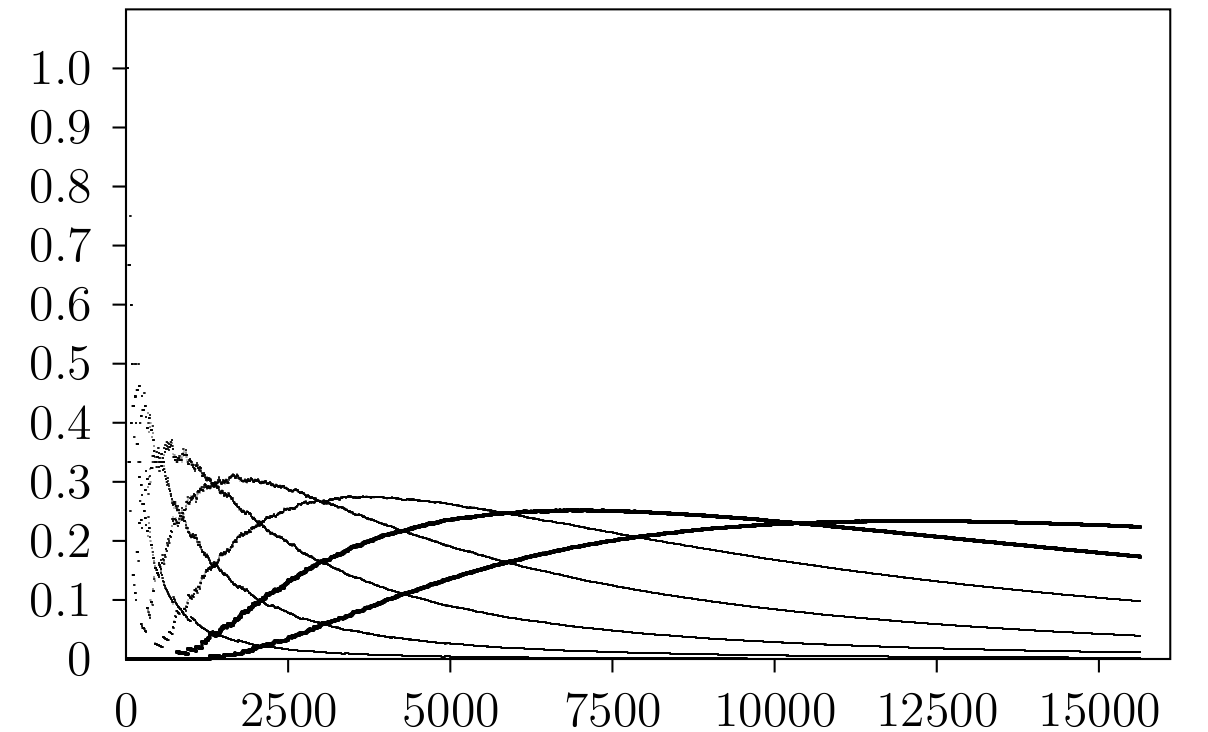
Recall that the prime number theorem says $\pi(q)\sim f_{P}(q)$ where $f_{P}(x)=x/\ln x$. Certainly $f_{P}:[3,\,\infty)\to\mathbb{R}$ has the required properties to be an interpolating function, so we expect $S_{i}^{P}(q)$ to have the behavior described above, at least for $i\geq 3$. Our data was generated using the first 100 odd primes (so the primes 3 through 547), producing complete information in the range $0<q\leq 550$ and up to homology dimension $16$. Figure 1a shows $S_{i}^{P}(q)$ versus $q$ for $0<q\leq 550$ and cell-dimensions $0\leq i\leq 6$; here our global expectations are closely exhibited: $S_{i}^{P}(q)$ is unimodal and as $i$ increases the maximum height decreases and the position of the maximum moves to the right. Figure 1b is a smoothing of $S_{i}^{P}(q)$, showing the quantity $S_{i,ave}^{P}(q)=\frac{1}{q}\sum_{k=1}^{q}S_{i}^{P}(k)$. The “double-line” effect evident in figure 1a occurs because we are summing odd numbers, so depending on the length of the sum only odd or even sums occur in each dimension.

As described in the introduction, the homology data of $Prime(q)$ encodes several classical arithmetic conjectures in number theory. In particular if $h_{1}^{P}(q)>0$ for all $q>8$ then the Goldbach conjecture holds, in fact in this case a stronger refinement of Goldbach holds, namely that every even number greater than or equal to 8 is the sum of two distinct odd primes. Our data is consistent with the stronger refinement of Goldbach and thus we conjecture:

The classical Goldbach conjecture is equivalent to the above conjecture holding for all even numbers greater than 3 and not equal to twice a prime. (The Goldbach conjecture is trivial for even numbers equal to twice a prime anyway.)

Figure 1c shows $H_{i}^{P}(q)$ for $0<q\leq 550$ and $0\leq i\leq 6$. Although appearing fairly scattered below $q\approx 100$ in these dimensions, the same global behavior as $S_{i}^{P}(q)$ manifests fairly rapidly as $q$ increases. As before, we also provide a smoothing of the data in figure 1d.

In general, the quantities $h_{i}^{P}(q)$ count the ways to sum to even or odd positive integers using $i+1$ distinct odd primes. Specifically if $h_{i}^{P}(q)>0$ for all sufficiently large $q$ and $i+1$ is even/odd, then all sufficiently large positive even/odd integers are expressible as a sum of distinct odd primes. At $i=2$ this is a refinement of the weak Goldbach conjecture that all odd numbers greater than 7 are a sum of three odd primes. The weak Goldbach conjecture has been shown to hold for almost all odd numbers by Vinogradav.

In our data $h_{2}^{P}(q)>0$ for $20\leq q\leq 550$ and so it is reasonable to conjecture:

Perhaps the most striking feature of the data is displayed in figure 2. Here, in a naive attempt to capture the expected asymptotic growth of $s_{i}^{P}(q)$, we graph $\left(s_{i}^{P}(q)\right)^{1/(i+1)}ln(q)$ versus $q$ for $0<q\leq 550$ and $0\leq i\leq 6$. In this range the data displays strong linearity. The data line with slope nearly one is the line for the zero-simplexes, the data line with the next greatest slope is the one-simplexes, and so-on. Note that since $\widehat{s}_{i}(q)\sim f_{P}(q)^{i+1}/(i+1)!=\frac{q^{i+1}}{ln(q)^{i+1}(i+1)!}$ by the prime number theorem and $\widehat{s}_{i}(\frac{q}{i+1})\leq s_{i}(q)\leq\widehat{s}_{i}(q)$, heuristically one might expect lines when plotting $\left(s_{i}^{P}(q)\right)^{1/(i+1)}\ln q$ versus $q$ with slopes roughly somewhere between $\frac{((i+1)!)^{-1/(i+1)}}{i+1}$ and $((i+1)!)^{-1/(i+1)}$. Running a least squares approximation on the data gives slopes of $0.632374$ when $i=1$; $0.404613$ when $i=2$; $0.284124$ when $i=3$; $0.211868$ when $i=4$; $0.164796$ when $i=5$; and $0.132366$ when $i=6$. These values are consistent with the heuristics. Thus it is reasonable to conjecture:

In this section we present data for the quota complexes $V(q)$ with $V=S=\{1,\,4,\,9,\,16,\ldots\}$ the set of squares, and $V=C=\{1,\,8,\,27,\,64,\ldots\}$ the set of cubes, which we denote $Square(q)$ and $Cube(q)$ respectively. We indicate the various functions of interest for these quota complexes with a superscript $S$ or $C$ as we did in section 3. Note that since $s_{0}^{S}(q)=\lfloor\sqrt{q-1}\rfloor-1$ and $s_{0}^{C}(q)=\lfloor\sqrt[3]{q-1}\rfloor-1$, our expectations for the global behavior of the families $S_{i}^{S}$ and $S_{i}^{C}$ are once again informed by proposition C.1.

Data for $Square(q)$ was generated using the first 25 squares, producing complete information for $0<q\leq 629$ and up to homology dimension 9. Figure 3a displays $S_{i}^{S}(q)$ for $0<q\leq 629$ and cell-dimensions $0\leq i\leq 6$. Here our expectations are strongly evident and are made all the more so in figure 3b which shows $S_{i,ave}^{S}(q)=\frac{1}{q}\sum_{k=1}^{q}S_{i}^{S}(k)$. The homology data $H_{i}^{S}(q)$ is notable for its lack of shape and is displayed in figure 3c. Finally, the heuristic growth of $s_{i}^{S}(q)$ as $q^{\frac{i+1}{2}}$ is verified in figure 3d as a graph of $s_{i}^{S}(q)^{\frac{2}{i+1}}$ versus $q$.

Data for $Cube(q)$ was generated using the first 25 cubes, producing complete information in the range $0<q\leq 15633$ and up to homology dimension 13. Once again our expectations are closely realized in the data: figure 4a shows $S_{i}^{C}(q)$ for $0\leq i\leq 6$ and figure 4b displays the growth of $s_{i}^{C}(q)$ as $q^{\frac{i+1}{3}}$. A graph of $H_{i}^{C}$ is not included as this data is scattered and apparently formless.

Based on the data, it is reasonable to conjecture:

In Section 3 we looked at the topology of the Prime complex $Prime(q)$ as the quota $q$ was varied. In this section we go back to that complex and consider the variance of another topological quantity, the Euler characteristic, of this complex as the quota $q$ changes.

Recall for a finite cell complex $X$, the Euler characteristic of $X$, $\chi(X)$, can be defined as an alternating sum of the number of cells of various dimensions. Namely, $\chi(X)=\sum_{j=0}^{\infty}(-1)^{j}c_{j}\in\mathbb{Z}$ where $c_{j}$ is the number of $j$-cells in the complex $X$. Recall that the Euler characteristic is a homotopy invariant, i.e., homotopy equivalent spaces have the same Euler characteristic.

Let us first consider, the unrestricted $Prime$ complex where $q=\infty$. This is an infinite dimensional simplex, but let us write down an (infinite) expression for its Euler characteristic. When restricted to the finite quota complexes $Prime(q)$, we will then get finite sum expressions for their Euler characteristic.

Recall the $j$-dimensional faces of the prime complex are in bijective correspondence with finite sets of $j+1$ distinct primes. Such a finite set of primes can be uniquely associated to its product by the unique factorization of integers. Thus the faces of the prime complex are in bijective correspondence with the square-free integers $>1$. (Recall an integer is square-free if no prime is repeated in its factorization).

Recall the Möbius function $\mu:\mathbb{N}\to\{-1,0,1\}$ is given by

Now note that for a $j$-cell of the prime complex, the corresponding square-free number $n$ will have $j+1$ distinct prime factors and so $\mu(n)=(-1)^{j+1}=-(-1)^{j}$. It is now easy to see that formally one has:

To get the corresponding finite sum expression for $\chi(Prime(q))$ we need to include the quota restriction which will allow only a finite number of the cells to be in $Prime(q)$. Well notice a $j$-face $[p_{0},p_{1},\dots,p_{j}]$ lies in $Prime(q)$ if and only if $\sum_{i=0}^{j}p_{i}<q$. Let us define $L_{q}:\mathbb{N}\to\{0,1\}$ by

Note that $L_{q}(n)=0$ for sufficiently large $n$ as there are only finitely many primes less than $q$ and finitely many square-free numbers with only those prime factors.

Then we have proven:

Note that as $q\to\infty$, $L_{q}$ converges pointwise to the characteristic function of the set of square-free integers.

In the data the Euler characteristic of $Prime(q)$ behaves very regularly as $q$ increases. Figure 5 displays the Euler characteristic for quotas $0<q\leq 550$. We will see in section 7 (example 3) that the growth of $\chi(Prime(q))$ with $q$ is subexponential.

In analytic number theory, one defines Merten’s function

By work of Titchmarsh it is known that the Riemann hypothesis that the nontrivial zeros of the Riemann zeta function lie on the critical line is equivalent to the statement that $M(N)=O(N^{0.5+\epsilon})$ for all $\epsilon>0$. In other words, for every $\epsilon>0$, there exists a constant $C=C(\epsilon)>0$ such that

for all $N$ large enough.

With this in mind we introduce a the $LogPrime$ complex which is the full quota complex ($q=\infty$) with vertices the set of primes where the weight of the vertex $p$ is $ln(p)$. Thus as a simplicial complex $LogPrime=Prime$ but $LogPrime(q)\neq Prime(q)$ for most finite quotas $q$.

References

- [A] T. M. Apostol Introduction to Analytic Number Theory, Undergraduate Texts in Mathematics, New York-Heidelberg: Springer-Verlag, 1976.
- [B] P. Billingsley Probability and Measure, Wiley, New York, 1986.
- [BBG] J. Borwein, D. Bailey, R. Girgensohn Experimentation in Mathematics: Computational Paths to Discovery, A K Peters, Wellesley, MA, 2004.
- [EH] H. Edelsbrunner, J. Harer, Persistant Homology - a Survey. In Surveys on discrete and computational geometry, volume 453 of Contemp. Math, pages 257-282. Amer. Math. Soc., Providence RI, 2008.
- [H] A. Hatcher Algebraic Topology Cambridge University Press, Cambridge 2002.
- [Ho] K. B. Howell Principles of Fourier Analysis Chapman & Hall/CRC, Boca Raton, FL, 2001.
- [Ka] M. Kahle Random Geometric Complexes to appear in Discrete & Computational Geometry.
- [LR] G. Latouche, V. Ramaswami Introduction to Matrix Analytic Methods in Stochastic Modelling, 1st ed. Chapter 1: Quasi-Birth-and-Death Processes; ASA SIAM, 1999.
- [Mu] J. R. Munkres Elements of algebraic topology Addison-Wesley, Menlo Park, CA, 1984.
- [PY] J. Pakianathan, E. Yalcin, On nilpotent ideals in the cohomology ring of a finite group, Topology 42, (2003), 1155-1183.
- [Ti] E .C. Titchmarsh The theory of the Riemann zeta-function, 2nd ed. revised by D.R. Heath-Brown, Oxford University Press, New York,1986.
- [Te] G. Tenenbaum Introduction to analytic and probabilistic number theory, Cambridge University Press, Cambridge 1995.
Dept. of Mathematics
University of Rochester,
Rochester, NY 14627 U.S.A.
E-mail address: jonpak@math.rochester.edu
E-mail address: winfree@math.rochester.edu