Multistability of free spontaneously-curved anisotropic strips

We start by considering a long rectangular plate whose length is much larger than its width $2a$, with the $x$ the coordinate along the direction parallel to the short edge and $y$ the coordinate along the direction parallel to the long edge (Figure 1). In practice we can consider the strip infinite along the $y$ direction to avoid dealing with end conditions. As noted by Mansifeld (1973), strips with aspect ratio five or more are already well described by this approximation.

The general constitutive equations for anisotropic plates can be expressed in terms of the ${\bf ABD}$ matrix (Ashton & Whitney 1970; Jones 1999), that relates the in-plane stresses ${\bf N}=(N_{x},N_{y},N_{xy})$ and out-of-plane moments ${\bf M}=(M_{x},M_{y},M_{xy})$ with the strain ${\boldsymbol{\epsilon}}=(\epsilon_{x},\epsilon_{y},\epsilon_{xy})$ and the difference ${\boldsymbol{\chi}}={\boldsymbol{\kappa}}-{\bf c}$ between the middle-surface curvatures¹¹ 1 We use Reissner’s notation for the twisting curvature, $\kappa_{xy}=-2\partial^{2}w/\partial x\partial y$, where $w$ is the height of the middle-surface above the $xy$ plane. ${\boldsymbol{\kappa}}=(\kappa_{x},\kappa_{y},\kappa_{xy})$ and their preferred (spontaneous) values ${\bf c}=(c_{x},c_{y},c_{xy})$, so that:

$$\left(\begin{array}[]{c}{\bf N}\\ {\bf M}\end{array}\right)=\left(\begin{tabular}[]{c|c}\phantom{-}{\bf A}&\phantom{-}{\bf B}\\ \hline\cr{\bf B}&{\bf D}\end{tabular}\right)\left(\begin{array}[]{c}{\boldsymbol{\epsilon}}\\ {\boldsymbol{\chi}}\end{array}\right)\,,$$

(1)

where ${\bf A}$ represents the extensional stiffness matrix, ${\bf D}$ is the bending stiffness matrix and ${\bf B}$ embodies the possible coupling between stretching and bending due to material anisotropy.

In terms of the strain, curvature and the material properties of the shell, the elastic energy density of a general anisotropic plate is given by (Mansfield 1989):

$$u=\frac{1}{2}(A_{ij}\epsilon_{i}\epsilon_{j}+2B_{ij}\chi_{i}\epsilon_{j}+D_{ij}\chi_{i}\chi_{j})$$

(2)

where the Einstein convention on repeated indices has been used, and the first and third terms are the stretching and bending energy densities while the second term characterizes the energy associated with the coupling between bending and stretching. Since it is often useful to know the constitutive equations (1) in their semi-inverted form, we write them as:

$$\left(\begin{array}[]{c}{\boldsymbol{\epsilon}}\\ {\bf M}\end{array}\right)=\left(\begin{tabular}[]{c|c}$\phantom{-}{\boldsymbol{\alpha}}$&$\hskip 3.44444pt{\boldsymbol{\beta}}\phantom{-}$\\ \hline\cr\\[-10.0pt] $-{\boldsymbol{\beta}}^{\rm T}$&$\,{\boldsymbol{\delta}}\phantom{-}$\end{tabular}\right)\left(\begin{array}[]{c}{\bf N}\\ {\boldsymbol{\chi}}\end{array}\right)\,,$$

(3)

where:

$${\boldsymbol{\alpha}}={\bf A}^{-1}\,,\qquad\quad{\boldsymbol{\beta}}=-{\bf A}^{-1}{\bf B}\,,\qquad\quad{\boldsymbol{\delta}}={\bf D}-{\bf B}{\bf A}^{-1}{\bf B}\,.$$

(4)

so the energy density (2) can be expressed in terms of ${\bf N}$ and $\boldsymbol{\chi}$ as:

$$u=\frac{1}{2}(\alpha_{ij}N_{i}N_{j}+\delta_{ij}\chi_{i}\chi_{j})\,.$$

(5)

In absence of body forces or external loads, the conditions for kinematical compatibility and mechanical equilibrium translate respectively into the following partial differential equations (Calladine 1993):

	$$\displaystyle\frac{\partial^{2}\epsilon_{x}}{\partial y^{2}}-\frac{\partial^{2}\epsilon_{xy}}{\partial x\,\partial y}+\frac{\partial^{2}\epsilon_{y}}{\partial x^{2}}=-\delta K\,,$$		(6a)
	$$\displaystyle\frac{\partial^{2}M_{x}}{\partial x^{2}}+2\frac{\partial^{2}M_{xy}}{\partial x\,\partial y}+\frac{\partial^{2}M_{y}}{\partial y^{2}}=\kappa_{x}N_{x}+\kappa_{xy}N_{xy}+\kappa_{y}N_{y}\,,$$		(6b)

where $\delta K=K-K_{0}$ is the difference between the Gaussian curvature of the deformed plate $K=\kappa_{x}\kappa_{y}-\kappa_{xy}^{2}$ and its spontaneous Gaussian curvature $K_{0}=c_{x}c_{y}-c_{xy}^{2}$. The radius of curvature of the strip is assumed to be much smaller than the typical length scale of the deformations (i.e. shallow shell approximation). This allows to simplify the differential structure of the theory by transforming covariant derivatives into standard partial derivatives. Eqs. 6 are then the classic Föppl-von Kármán plates equations expressed in terms of stress and curvature. Since the strip is assumed to be infinitely long in the $y$ direction, all physical quantities should be invariant with respect to translations along $y$. Mechanical equilibrium requires ${\nabla\cdot}\,{\bf N}=0$, which together with the condition of translational invariance along $y$ yields:

$$\frac{\partial N_{x}}{\partial x}=\frac{\partial N_{xy}}{\partial x}=0\,.$$

In absence of applied forces along the edges this implies $N_{x}=N_{xy}=0$. In addition, the Mainardi-Codazzi compatibility equations $\nabla_{i}\kappa_{jk}=\nabla_{k}\kappa_{ij}$ yield:

$$\frac{\partial\kappa_{x}}{\partial y}-\frac{\partial\kappa_{xy}}{\partial x}=0\,,\qquad\qquad\frac{\partial\kappa_{y}}{\partial x}-\frac{\partial\kappa_{xy}}{\partial y}=0\,,$$

that, together with the condition of translational invariance along $y$, imply that $\kappa_{y}$ and $\kappa_{xy}$ are both constant. Thus, equations (6) simplify to:

	$$\displaystyle\frac{\partial^{2}\epsilon_{y}}{\partial x^{2}}=-\delta K\,,$$		(7a)
	$$\displaystyle\frac{\partial^{2}M_{x}}{\partial x^{2}}=\kappa_{y}N_{y}\,.$$		(7b)

Using the semi-inverted constitutive equations (3), one can easily rewrite (7) in the form of a single differential equation for the transverse moment $M_{x}$. To do this we start by writing:

	$$\displaystyle\epsilon_{y}=\alpha_{22}N_{y}+\beta_{21}\chi_{x}+\beta_{22}\chi_{y}+\beta_{26}\chi_{xy}\,,$$		(8a)
	$$\displaystyle M_{x}=-\beta_{21}N_{y}+\delta_{11}\chi_{x}+\delta_{12}\chi_{y}+\delta_{16}\chi_{xy}\,.$$		(8b)

Then, inverting (8b) and using (7b) we get:

	$$\displaystyle\kappa_{x}=c_{x}+\frac{1}{\delta_{11}}\left(M_{x}+\frac{\beta_{21}}{\kappa_{y}}\frac{\partial^{2}M_{x}}{\partial x^{2}}-\delta_{12}\chi_{y}-\delta_{16}\chi_{xy}\right)\,,$$		(9a)
	$$\displaystyle\frac{\partial^{2}\kappa_{x}}{\partial x^{2}}=\frac{1}{\delta_{11}}\left(\frac{\partial^{2}M_{x}}{\partial x^{2}}+\frac{\beta_{21}}{\kappa_{y}}\frac{\partial^{4}M_{x}}{\partial x^{4}}\right)\,.$$		(9b)

Combining these two equations with (7) we finally obtain:

$$(\alpha_{22}\delta_{11}+\beta_{21}^{2})\,\frac{\partial^{4}M_{x}}{\partial x^{4}}+2\beta_{21}\kappa_{y}\frac{\partial^{2}\,M_{x}}{\partial x^{2}}+\kappa_{y}^{2}M_{x}\\[7.0pt] =\kappa_{y}\left\{\delta_{11}(c_{x}c_{y}-c_{xy}^{2}+\kappa_{xy}^{2})+\kappa_{y}[\delta_{12}(\kappa_{y}-c_{y})+\delta_{16}(\kappa_{xy}-c_{xy})-\delta_{11}c_{x}]\right\}\,.\\$$

(10)

The boundary conditions associated with equations (7) for a strip with no applied forces and torques at the lateral edges have been discussed by Reissner (1993) and translate into the requirement:

$$M_{x}=\frac{\partial M_{x}}{\partial x}=0\qquad x=\pm a\,.$$

(11)

Together, (10) and (11) complete the formulation of the boundary value problem for the behavior of a long anisotropic strip with spontaneous curvature and twist.

Before we go further, it is useful to review the different form of elastic anisotropy, following the theory of laminates (Jones 1999). Various forms of matrix coupling the in-plane strain to the out-of-plane curvature ${\bf B}$ can be obtained by controlling the relative orientation of the laminae forming the layers of a composite plate. Thus in a cross-ply fiber reinforced composite, in which the fibers in each layer are alternatively oriented at 0^∘ and 90^∘ with respect to the $y$ axis of the strip, one has:

$${\bf B}=\left(\begin{array}[]{ccc}B_{11}&0&0\\ 0&-B_{11}&0\\ 0&0&0\end{array}\right)\,.$$

(12)

with $B_{11}=E_{\perp}h^{2}(E_{\parallel}/E_{\perp}-1)/4P$, where $E_{\parallel}$ and $E_{\perp}$ are the Young moduli in the parallel and transverse directions of the fiber and $P$ is the number of layers of the laminate. Antisymmetric angle-ply laminates, on the other hand, have laminae oriented as same angle $\theta$ with respect to the laminate coordinate axis on one side of the middle-surface and the corresponding equal thickness laminae oriented at $-\theta$ on the other side at the same distance form the middle-surface. In this case:

$${\bf B}=\left(\begin{array}[]{ccc}0&0&B_{16}\\ 0&0&B_{26}\\ B_{16}&B_{26}&0\end{array}\right)\,.$$

(13)

General asymmetric laminates obtained by the asymmetric stacking of isotropic layers with different material properties about the middle-surface, have finally:

$${\bf B}=\left(\begin{array}[]{ccc}B_{11}&B_{12}&0\\ B_{12}&B_{22}&0\\ 0&0&B_{66}\end{array}\right)\,.$$

(14)

In the next section we start with a focus on the case of orthotropic strips for which $B_{ij}=0$, while the case of angle-ply laminates is discussed in Section 4 in the context of tristable strips.

In the case of naturally flat strips with no coupling between stretching and bending (i.e. $B_{ij}=0$ and $\delta_{ij}=D_{ij}$), equation (10) reduces to the equation given by Reissner (1993) for the case of a inhomogeneous anisotropic strip:

$$\alpha_{22}\,\frac{\partial^{4}M_{x}}{\partial x^{4}}+\frac{\kappa_{y}}{D_{11}}\,M_{x}=\kappa_{y}\,\frac{D_{12}\kappa_{y}^{2}+D_{16}\kappa_{y}\kappa_{xy}+D_{11}\kappa_{xy}^{2}}{D_{11}}\,.$$

Now, letting:

$$\displaystyle\varphi_{1}=-\frac{\beta_{21}\kappa_{y}}{\alpha_{22}\delta_{11}+\beta_{21}^{2}}\,,\qquad\varphi_{2}=\frac{\kappa_{y}^{2}}{\alpha_{22}\delta_{11}+\beta_{21}^{2}}$$

and:

$$\varphi_{3}=\frac{\kappa_{y}\left\{\delta_{11}(c_{x}c_{y}-c_{xy}^{2}+\kappa_{xy}^{2})+\kappa_{y}[\delta_{12}(\kappa_{y}-c_{y})+\delta_{16}(\kappa_{xy}-c_{xy})-\delta_{11}c_{x}]\right\}}{\alpha_{22}\delta_{11}+\beta_{21}^{2}}\,,$$

the solution of equation (10) which satisfies the homogeneous boundary conditions (11) is given by:

$$M_{x}=-\delta_{11}(\kappa-\kappa_{0})+\delta_{11}C_{1}\cosh k_{1}x\cos k_{2}x+\delta_{11}C_{2}\sinh k_{1}x\sin k_{2}x\,,$$

(15)

where:

	$$\displaystyle\kappa_{0}=\frac{(c_{x}c_{y}-c_{xy}^{2})+\kappa_{xy}^{2}}{\kappa_{y}}\,,$$		(16a)
	$$\displaystyle\kappa=c_{x}+\frac{\delta_{12}}{\delta_{11}}(c_{y}-\kappa_{y})+\frac{\delta_{16}}{\delta_{11}}(c_{xy}-\kappa_{xy})\,.$$		(16b)

and:

	$$\displaystyle C_{1}=(\kappa-\kappa_{0})\,\left(\frac{k_{1}\cosh ak_{1}\sin ak_{2}+k_{2}\sinh ak_{1}\cos ak_{2}}{k_{1}\sin ak_{2}\cos ak_{2}+k_{2}\sinh ak_{1}\cosh ak_{1}}\right)\,,$$		(17a)
	$$\displaystyle C_{2}=(\kappa-\kappa_{0})\,\left(\frac{k_{2}\cosh ak_{1}\sin ak_{2}-k_{1}\sinh ak_{1}\cos ak_{2}}{k_{1}\sin ak_{2}\cos ak_{2}+k_{2}\sinh ak_{1}\cosh ak_{1}}\right)\,,$$		(17b)

with:

$$k_{1}=\left(\frac{\sqrt{\varphi_{2}}+\varphi_{1}}{2}\right)^{\frac{1}{2}}\,,\qquad k_{2}=\left(\frac{\sqrt{\varphi_{2}}-\varphi_{1}}{2}\right)^{\frac{1}{2}}\,,$$

The longitudinal stress $N_{y}$ and the transverse curvature $\kappa_{x}$ can be readily calculated by replacing $M_{x}$ in equations (7b) and (9a). This yields:

$$N_{y}=\delta_{11}C_{2}^{\prime}\cosh k_{1}x\cos k_{2}x-\delta_{11}C_{1}^{\prime}\sinh k_{1}x\sin k_{2}x\,,$$

(18)

with:

$$C_{1}^{\prime}=\frac{(\alpha_{22}\delta_{11})^{\frac{1}{2}}C_{1}+\beta_{21}C_{2}}{\alpha_{22}\delta_{11}+\beta_{21}^{2}}\,,\qquad C_{2}^{\prime}=\frac{(\alpha_{22}\delta_{11})^{\frac{1}{2}}C_{2}-\beta_{21}C_{1}}{\alpha_{22}\delta_{11}+\beta_{21}^{2}}\,,$$

and finally:

$$\kappa_{x}=\kappa_{0}+(C_{1}+\beta_{21}C_{2}^{\prime})\cosh k_{1}x\cos k_{2}x+(C_{2}-\beta_{21}C_{1}^{\prime})\sinh k_{1}x\sin k_{2}x\,.$$

(19)

Eq. (19) is equivalent to an expression given by Galletly & Guest (2004b) for the case of a bistable composite slit tube. We will now examine the effect of spontaneous curvature and elastic anisotropy on the energy landscape of elastic strips.

To understand the energy landscape of the strip, we analyze the total elastic energy $\hat{U}$ given by (22) and (23). We first focus on configurations having constant transverse curvature $\hat{\kappa}_{x}$: if $\hat{\kappa}_{y}$ is nonzero, from equation (17) and (20a) it follows that $C_{1}=C_{2}=0$ and $\hat{\kappa}=\hat{\kappa}_{0}$. This solution has zero longitudinal stress and, as a consequence, is an isometry of the base configuration: a deformation that preserves the local metric of the shell so that $\boldsymbol{\epsilon}=\boldsymbol{0}$. The latter statement can be also verified by calculating the Gaussian curvature of the deformed strip. Since $\hat{\kappa}_{x}=\hat{\kappa}=\hat{\kappa}_{0}$, equation (16a) yields:

$$\hat{\kappa}_{x}=\frac{(\hat{c}_{x}\hat{c}_{y}-\hat{c}_{xy}^{2})+\hat{\kappa}_{xy}^{2}}{\hat{\kappa}_{y}}\,,$$

(25)

which implies that $\hat{\kappa}_{x}\hat{\kappa}_{y}-\hat{\kappa}_{xy}^{2}=\hat{c}_{x}\hat{c}_{y}-\hat{c}_{xy}^{2}$ as required by Gauss’ theorema egregium (Kreyszig 1991). The corresponding total elastic energy per unit length $\hat{U}$ is given by:

$$\hat{U}=\frac{\hat{t}^{2}}{12}\,[\beta(\hat{\kappa}_{y}-\hat{c}_{y})^{2}+\rho(\hat{\kappa}_{xy}-\hat{c}_{xy})^{2}]\,.$$

(26)

The condition $\hat{\kappa}=\hat{\kappa}_{0}$ used to obtain the isometric solution (25) describes, in the plane $(\hat{\kappa}_{y},\hat{\kappa}_{xy})$ a continuous set of configurations of zero stretching energy. The explicit form of this geometrical locus is given by:

$$\nu\hat{\kappa}_{y}^{2}+\hat{\kappa}_{xy}^{2}-(\hat{c}_{x}+\nu\hat{c}_{y})\hat{\kappa}_{y}=\hat{c}_{xy}^{2}-\hat{c}_{x}\hat{c}_{y}\,,$$

(27)

that corresponds to an ellipse with focii at :

$$\hat{\kappa}_{y,\,0}=\frac{1}{2\nu}\,(\hat{c}_{x}+\nu\hat{c}_{y})\,,\qquad\hat{\kappa}_{xy,\,0}=0\,,$$

and semi-axes $a_{y}=1/\ell\sqrt{\nu}$ and $a_{xy}=1/\ell$ with $\ell^{-2}=\frac{1}{4\nu}(\hat{c}_{x}-\nu\hat{c}_{y})^{2}+\hat{c}_{xy}^{2}$. The bending energy, however, suppresses this soft mode by selecting a minimum in this class of isometric deformations: the base configuration having $\hat{\kappa}_{y}=\hat{c}_{y}$ and $\hat{\kappa}_{xy}=\hat{c}_{xy}$.

A special but not necessarily isometric solution with constant curvature can be found by taking the limit $\hat{\kappa}_{y}\rightarrow 0$ of equation (20a) which gives:

$$\hat{\kappa}_{x}=\hat{c}_{x}+\nu\hat{c}_{y}\,.$$

(28)

The corresponding longitudinal stress is given then by:

$$\hat{N}_{y}=\frac{\hat{t}}{6}\,\beta\,(3\hat{x}^{2}-1)[(\hat{c}_{x}\hat{c}_{y}-\hat{c}_{xy}^{2})+\hat{\kappa}_{xy}^{2}]\,,$$

(29)

using which we can calculate the total elastic energy as:

$$\hat{U}=\beta\left\{\frac{1}{45}\,[(\hat{c}_{x}\hat{c}_{y}-\hat{c}_{xy}^{2})+\hat{\kappa}_{xy}^{2}]^{2}+\frac{\hat{t}^{2}}{12}\,\left[\hat{c}_{y}^{2}+\frac{\rho}{\beta}\,(\hat{\kappa}_{xy}-\hat{c}_{xy})^{2}\right]\right\}\,.$$

(30)

This class of deformations belongs to the set of isometries only when the first term in the left-hand side of equation (30) vanishes, namely when:

$$\hat{\kappa}_{xy}^{2}=\hat{c}_{xy}^{2}-\hat{c}_{x}\hat{c}_{y}=-\hat{K}_{0}\,.$$

(31)

Clearly this is possible only when the initial Gaussian curvature $\hat{K}_{0}$ is negative or zero. In the latter case the strip has only one minimum corresponding to the base configuration (see right of Figure 2).

However, a secondary equilibrium configuration of constant curvature is obtained if $\hat{c}_{x}=\hat{c}_{y}=0$ and $\hat{c}_{xy}\neq 0$, when Eq. (30) reads:

$$\hat{U}=\beta\left\{\frac{1}{45}\,(\hat{\kappa}_{xy}^{2}-\hat{c}_{xy}^{2})^{2}+\frac{\hat{t}^{2}}{12}\frac{\rho}{\beta}\,(\hat{\kappa}_{xy}-\hat{c}_{xy})^{2})\right\}\,.$$

(32)

Then, in addition to the base configuration $\hat{\kappa}_{xy}=\hat{c}_{xy}$, the energy has a secondary minimum corresponding to the twisting curvature:

$$\hat{\kappa}_{xy}=-\frac{1}{2}\left\{\hat{c}_{xy}+\sqrt{\hat{c}_{xy}^{2}-\frac{15}{2}\,(\rho/\beta)\,\hat{t}^{2}}\right\}\,,$$

(33)

which is approximately $\hat{\kappa}_{xy}\approx-\hat{c}_{xy}$ (see Figure 2, left). The stability of the secondary minimum depends on $\rho$, $\beta$ as well as the Poisson ratio $\nu$. To assess this, we calculate the components of the Hessian matrix:

	$$\displaystyle\frac{\partial^{2}\hat{U}}{\partial\hat{\kappa}_{y}^{2}}=\beta\left\{\frac{\hat{t}^{2}}{6}+\frac{4}{45}\nu\,(\hat{\kappa}_{xy}^{2}-\hat{c}_{xy}^{2})+\frac{16}{945}\frac{(\nu^{2}-\beta)}{\hat{t}^{2}}(\hat{\kappa}_{xy}^{2}-\hat{c}_{xy}^{2})^{2}\right\}\,,$$
	$$\displaystyle\frac{\partial^{2}\hat{U}}{\partial\hat{\kappa}_{y}\partial\hat{\kappa}_{xy}}=0\,,\qquad\qquad\frac{\partial^{2}\hat{U}}{\partial\hat{\kappa}_{xy}^{2}}=-\frac{4}{45}\beta\,(\hat{c}_{xy}^{2}-3\kappa_{xy}^{2})+\frac{\hat{t}^{2}}{6}\rho\,,$$

where $\hat{\kappa}_{xy}$ is given by Eq. (33). In order for the secondary minimum to be stable, the eigenvalues of the Hessian matrix must be positive. Upon expanding $\partial^{2}\hat{U}/\partial\hat{\kappa}_{y}^{2}$ at the second order in $\hat{t}$, this condition reduces to the following inequality:

$$\beta-2\nu\rho-\frac{10}{7}\left(1-\frac{\nu^{2}}{\beta}\right)\rho^{2}>0\,.$$

This implies the following requirment on $\rho$:

$$\rho<\frac{\beta}{\nu+\sqrt{\frac{10\beta-3\nu^{2}}{7}}}\,.$$

(34)

In summary, strips having zero spontaneous principal curvatures $\hat{c}_{x}=\hat{c}_{y}=0$ and non-zero spontaneous twist $\hat{c}_{xy}$, admit a secondary equilibrium configuration where the principal curvatures vanish, i.e. $\hat{\kappa}_{x}=\hat{\kappa}_{y}=0$ while the twisting curvature is reversed $\hat{\kappa}_{xy}\approx-\hat{c}_{xy}$. The secondary minimum is stable for low enough shear modulus, a scenario previously discussed by Seffen (2007) for the case of an elliptical plate endowed with pure twist. The most important difference between the two cases is that here the strip has zero bending moment along the lateral edges unlike the plate investigated by Seffen which can support a finite bending moment at the boundary. As a consequence the transverse curvature $\hat{\kappa}_{x}$, which is a free parameter in uniform curvature models, is here adjusted in order to maintain the boundary moment-free and this severely restricts the space of possible uniform curvature configurations.

The previous situation is an example of bistability in a strip with a negative spontaneous Gaussian curvature $\hat{K}_{0}=-\hat{c}_{xy}^{2}$, where the principal curvatures $\hat{c}_{x}$ and $\hat{c}_{y}$ vanish identically while the surface is purely twisted. However when $\hat{c}_{x}\hat{c}_{y}\neq 0$ and $\hat{K}_{0}<0$, the strip also exhibits a secondary equilibrium configuration, albeit with a variable transverse curvature $\hat{\kappa}_{x}$ discussed in the next section.

When the constraint of constant curvature is lifted, new minima appear in the energy landscape. Figure 3 shows a contour plot of the total elastic energy in the plane $(\hat{\kappa}_{x},\,\hat{\kappa}_{xy})$ for the two cases $\hat{c}_{x}\hat{c}_{y}>0$ (left), $\hat{c}_{x}\hat{c}_{y}<0$ (right) and $\hat{c}_{xy}=0$ in both case. For positive spontaneous Gaussian curvatures the energy minima are those described in the previous section when $\hat{\kappa}_{xy}=0$.

The transverse curvature $\hat{\kappa}_{x}$ associated with the secondary minimum at $\hat{\kappa}_{y}<0$ is mostly constant across the width of the strip and equal to

$$\hat{\kappa}_{0}=\frac{(\hat{c}_{x}\hat{c}_{y}-\hat{c}_{xy}^{2})+\hat{\kappa}_{xy}^{2}}{\hat{\kappa}_{y}}\,,$$

with exception for a boundary layer (Figure 4). This phenomenon, first noted by Lamb (1891), is due to the rapid build-up of the bending moment $M_{x}$ from zero at the edges to a non-zero value that inevitably develops in any configuration other than the base state (see Mansfield 1989 for a detailed explanation). An estimate of the size of the boundary layer is given by $1/k\approx(t/|\kappa_{y}|)^{\frac{1}{2}}$; however it vanishes in a strip of lenticular cross section whose thickness (hence the bending moment) smoothly tapers and vanishes at the edges.

On on the other hand, for negative Gaussian curvature $\hat{c}_{x}\hat{c}_{y}<0$ and $\hat{c}_{xy}=0$, the secondary minimum becomes a saddle point and the elastic energy has only one minimum corresponding to the base configuration. It is interesting to notice, in this latter case, that the regions of positive and negative $\hat{\kappa}_{y}$ of the energy landscape are separated by a barrier of height $\hat{U}(\hat{\kappa}_{y}=0)\sim\hat{K}_{0}^{2}$ that is large everywhere with exception for two “passes” at $\hat{\kappa}_{xy}=\pm(-\hat{c}_{x}\hat{c}_{y})^{1/2}$ (see Figure 5). The existence of these passes along the energy barrier at $\hat{\kappa}_{y}=0$ is the reason for the non-existence of a secondary equilibrium configuration in strips with spontaneous negative Gaussian curvature. As explained in the previous section and summarized in equation (31), the stretching energy associated with the barrier at $\hat{\kappa}_{y}=0$ scales like $\hat{U}_{s}\sim(\hat{K}_{0}+\hat{\kappa}_{xy}^{2})^{2}$ and, in presence of spontaneous negative Gaussian curvature, it can be relieved through twist. This leads to the formation of passes at $\hat{\kappa}_{xy}=\pm(-\hat{K}_{0})^{1/2}$ shown in Figure 3 and 5 which allow the transverse curvature $\hat{\kappa}_{y}$ to be switched from positive to negative (and vice versa) isometrically. Positive spontaneous Gaussian curvatures, on the other hand, cannot be accommodated through twist and thus there are no passages across the energy barrier at $\hat{\kappa}_{y}=0$; consequently there is a secondary minimum.

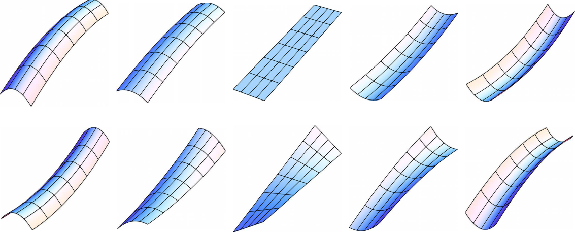
To get an intuitive sense of these passes in the energy landscape, imagine a strip of positive spontaneous Gaussian curvature (upper left frame of Figure 6). To evert the strip, one choice is to flatten the strip and then reverse its curvature. Since the strip is naturally curved, the intermediate flat conformation will suffer a large strain and this corresponds to the large energy barrier shown in Figure 5. On the other hand, if the strip is naturally shaped like a saddle (bottom left frame of Figure 6), turning the strip inside-out can be achieved by pulling apart two opposite corners until the strip is fully extended and maximally twisted, and then bend it into the new configuration. The latter deformation can be performed without stretching the surface and thus with no energy cost other than bending, in contrast with the case of a strip with positive $\hat{K}_{0}$. Similar deformation pathways have been analyzed by Fernandes et al. (2010) as possible strategies to achieve shape control of bistable composite plates using embedded actuators.

However, when strips with negative spontaneous Gaussian curvature $\hat{K}_{0}<0$ have a non-zero spontaneous twist $\hat{c}_{xy}$, they admit bistable configurations. In addition to the configuration with constant curvature described in the previous section in the special case $\hat{c}_{x}=\hat{c}_{y}=0$ and $\hat{c}_{xy}\neq 0$, another configuration can be obtained by setting $\hat{c}_{x}\hat{c}_{y}\neq 0$ with $\hat{K}_{0}<0$. Figure 7 shows a contour plot of the total elastic energy (22) and (23) of a strip with $\hat{c}_{x}=2$, $\hat{c}_{y}=1$ and $\hat{c}_{xy}=2$, thus $\hat{K}_{0}=-2$. The plot on the left (in which $\beta=10$) shows a secondary minimum in the proximity of the point $(\hat{\kappa}_{y},\,\hat{\kappa}_{xy})=(\hat{c}_{y},\,-\hat{c}_{xy})$. When anisotropy parameter $\beta$ is decreased, however, the secondary minimum disappears and the energy landscape is again characterized by a unique minimum corresponding to the base configuration.

Such a configuration has energy $\hat{U}\approx(\rho/\beta)\,\hat{c}_{xy}^{2}$, and has a minimum for large values of $\beta/\rho$. One might expect that the value of $\beta/\rho$ necessary to have a secondary minimum of this kind would increase monotonically with $\hat{c}_{xy}$; however this is incorrect. In Figure 4 we show the “phase diagram” of the monostability/bistability region for a strip with spontaneous curvatures $\hat{c}_{x}=2$ and $\hat{c}_{y}=1$ in the plane $(\beta/\rho,\,\hat{c}_{xy})$. Upon fixing the spontaneous twist $\hat{c}_{xy}$, the bistability region can be accessed by increasing $\beta/\rho$ as expected. However, for fixed $\beta/\rho$, the bistable region is accessed by increasing the spontaneous twist. The origin of this behavior is related with the height of the energy barrier at $\hat{\kappa}_{y}=0$ separating the secondary minimum from the basin of attraction of the base configuration at $\hat{\kappa}_{y}<0$. From equation (30) we see that the height of such a barrier $\hat{U}\approx\beta\hat{K}_{0}^{2}$. For fixed $\beta/\rho$, decreasing $\hat{c}_{xy}$ (or equivalently $|\hat{K}_{0}|$) will lower the height of the barrier until the basin of attraction associated with the portion where $\hat{\kappa}_{y}<0$ of the base configuration will merge with that of the secondary minimum. For values of $\hat{c}_{xy}$ smaller than this critical value, the energy landscape is then characterized by a unique minimum (i.e. the base configuration) surrounded by a large C-shaped basin of attraction that starts from the base configuration and extends in the region $\hat{\kappa}_{y}<0$ penetrating the barrier at $\hat{\kappa}_{y}=0$ through the passes located at $\hat{\kappa}_{xy}=\pm(-\hat{K}_{0})^{1/2}$ (see right of Figure 7). Once again, the presence of two regions across the barrier at $\hat{\kappa}_{y}=0$ where the stretching energy drops, plays a crucial role in assuring the existence of bistable configurations.

In summary, orthotropic strips exhibit various form of bistability depending to their spontaneous curvature and elastic moduli. The simplest bistable configurations have constant curvature throughout the width of the strip and correspond to isometries of the base configuration. Non-isometric secondary equilibria have, on the other hand, variable transverse curvature $\hat{\kappa}_{x}$; this is approximately constant and equal to $\hat{\kappa}_{0}=(\hat{K}_{0}+\hat{\kappa}_{xy}^{2})/\hat{\kappa}_{y}$ in the bulk of the strip, but abruptly jumps to $\hat{\kappa}=\hat{c}_{x}+\nu(\hat{c}_{y}-\hat{\kappa}_{x})$ near the edges to relieve the bending moment that forms in the bulk when the strip is in a configuration different from the base one. For strips with positive spontaneous Gaussian curvature, in particular, the secondary equilibrium configuration has transverse curvature of opposite sign relative to the base configuration. Strips with negative spontaneous Gaussian curvature, on the other hand, do not possess a secondary equilibrium configuration unless they have sufficient spontaneous twist $\hat{c}_{xy}$. The existence of bistability in this case also relies on the value of the ratio $\beta/\rho$ between the Young’s modulus along the longitudinal direction and the shear modulus. Figure 8 shows a phase-diagram of the monostability/bistability regions in in the plane $(\hat{c}_{x},\,\hat{c}_{y})$ for strips of various spontaneous twist $\hat{c}_{xy}$.

As we mentioned in the introduction of Section 3, the requirement for the matrices ${\bf A}$ and ${\bf D}$ to be positive definite translates into the conditions $\beta>\nu^{2}$ and $\rho>0$. In this section we show that when the limit $\beta\rightarrow\nu^{2}$ is approached, a new stable minimum appears in the energy landscape of the configurations allowing for tristability. The presence of three minima in the reduced quasi-one-dimensional geometry of elastic strips complements the appearance of such a landscape for corrugated strips, where tristability arises as the consequence of the coupling between internal prestresses created while imprinting the corrugation and non-linear geometrical changes during deformation (Norman et al. 2008).

Letting $\beta=\nu^{2}+\epsilon$ and expanding equations (22) and (23) in powers of $\epsilon$ gives:

$$\hat{U}=\nu^{2}\bigg\{\frac{1}{45}\,\left[(\hat{\kappa}_{y}-\hat{c}_{y})(\nu\hat{\kappa}_{y}-\hat{c}_{x})+\hat{\kappa}_{xy}^{2}-\hat{c}_{xy}^{2}\right]^{2}\\ +\frac{1}{12}\,\hat{t}^{2}\left[(\hat{\kappa}_{y}-\hat{c}_{y})^{2}+\frac{\rho}{\nu^{2}}\,(\hat{\kappa}_{xy}^{2}-\hat{c}_{xy}^{2})\right]\bigg\}+o(\epsilon)\,.$$

(35)

Then, with $\hat{\kappa}_{xy}=\hat{c}_{xy}$, it is easy to prove that $\partial\hat{U}/\partial\hat{\kappa}_{y}=0$ when $\hat{\kappa}_{y}=\hat{c}_{y}$ and also when:

$$\hat{\kappa}_{y}^{\pm}=\frac{1}{4}\left\{\hat{c}_{y}+\frac{1}{\nu}\left[3\hat{c}_{x}\pm\sqrt{(\hat{c}_{x}-\nu\hat{c}_{y})^{2}-30\,\hat{t}^{2}}\,\right]\right\}\,.$$

(36)

Thus, in addition to the base configuration and the secondary minimum at $\hat{\kappa}_{y}<0$ discussed in section (3.2), the energy has a third minimum at $\hat{\kappa}_{y}=\hat{\kappa}_{y}^{+}$ while $\hat{\kappa}_{y}^{-}$ is the location of the maximum separating the third minimum from the base configuration. For relatively thin shells, $\hat{t}\ll 1$ so that one finds simply $\hat{\kappa}_{y}^{+}\approx\hat{c}_{x}/\nu$ and $\hat{\kappa}_{y}^{-}\approx(\hat{c}_{y}+\hat{c}_{x}/\nu)/2$. The energy of the third minimum is given approximately by:

$$\hat{U}(\hat{\kappa}_{y}^{+})\approx\frac{1}{12}\,\hat{t}^{2}\nu^{2}\left(\hat{c}_{y}-\frac{\hat{c}_{x}}{\nu}\right)^{2}$$

(37)

Figure 9 shows a contour plot of the total elastic energy per unit length $\hat{U}$ from (22) and (23) for $\hat{c}_{x}=1$, $\hat{c}_{y}=2$, $\hat{c}_{xy}=0$ and $\beta=\nu^{2}+10^{-2}$, with $\nu=1/3$ and $\rho=1$. The primary, secondary and tertiary minima are indicated with the letters $P$, $S$ and $T$ respectively.

In the limit $\beta\rightarrow\nu^{2}$, tristability has been noted by Vidoli & Maurini (2009) in the case of plates with free boundaries and uniform curvature, although the physical origins of this phenomenon were not discussed. In our simple setting, consistent with the arguments in section (3.1), there is a continuous set of configurations of zero stretching energy corresponding to the isometries of the base state. In the plane $(\hat{\kappa}_{y},\,\hat{\kappa}_{xy})$ this set describes an ellipse whose intersections with the $\hat{\kappa}_{y}$ axis (i.e. the untwisted configurations) are given by $\hat{\kappa}_{y}=\hat{c}_{y}$ and $\hat{\kappa}_{y}=\hat{c}_{x}/\nu$. The small but finite bending stiffness along the principal directions prevents this from being a true zero energy mode and instead leads to the existence of a soft mode by raising the energy of the minimum at $\hat{\kappa}_{y}=\hat{c}_{x}/\nu$; for $\beta\gg\nu^{2}$ (i.e. $D_{22}\gg D_{11}$) the minimum is completely suppressed. Taking the limit $\beta\rightarrow\nu^{2}$ corresponds to lowering the bending stiffness so that the energies of the two isometric configurations $\hat{\kappa}_{y}=\hat{c}_{y}$ and $\hat{\kappa}_{y}=\hat{c}_{x}/\nu$ are comparable again. This mechanism is completely general and independent of the specific geometry of the problem; any plate with shallow spontaneous curvature is amenable to a set of isometries and multistability can be in principle obtained by setting $\det({\bf D})\sim 0$, which in the case of orthotropic plates corresponds in fact to $\beta\sim\nu^{2}$.

An interesting feature of this tristable energy landscape relies on the fact that the energy barrier separating the minima at $\hat{\kappa}_{y}=\hat{c}_{y}$ and $\hat{\kappa}_{y}=\hat{c}_{x}/\nu$ is generally much smaller than that located at $\hat{\kappa}_{y}=0$ separating the base configuration with the minimum at $\hat{\kappa}_{y}<0$. More precisely:

$$\hat{U}(\hat{\kappa}_{y}^{-})\approx\frac{1}{720}\,(\hat{c}_{x}-\nu\hat{c}_{y})^{4}$$

(38)

while $\hat{U}(0)\approx(1/45)\,(\nu\hat{K}_{0})^{2}$. Assuming $\hat{\kappa}_{xy}=\hat{c}_{xy}=0$, the ratio between the height of these two energy barriers can be approximated as:

$$\frac{\hat{U}(\hat{\kappa}_{y}^{-})}{\hat{U}(0)}\approx\frac{1}{16}\left[\left(\frac{\hat{c}_{x}}{\nu\hat{c}_{y}}\right)+\left(\frac{\hat{c}_{x}}{\nu\hat{c}_{y}}\right)^{-1}-2\right]^{2}=\left[\sinh\frac{1}{2}\log\left(\frac{\hat{c}_{x}}{\nu\hat{c}_{y}}\right)\right]^{4}\,,$$

(39)

Assuming $\hat{c}_{x}<\hat{c}_{y}$, this ratio is $O(10^{-2})$. For $\hat{c}_{x}>\hat{c}_{y}$ the previous relation is no longer valid as the bending energy, that was neglected to derive (39) becomes relevant; however, the order of magnitude of the ratio $\hat{U}(\hat{\kappa}_{y}^{-})/\hat{U}(0)$ remains always of order $O(10^{-2})$.

References

- [2] Abdulrahim, M., Garcia, H. & Lind, R. 2005 Flight characteristics of shaping the membrane wing of a micro air vehicle. J. Aircraft 42, 131-137.
- [4] Ashton, J. E. & Whitney, J. E. 1970 Theory of laminated plates, Progress in materials science series vol. 4. Stamford, CT: Technomic.
- [6] Calladine, C. R. 1993 Theory of shell structures. Cambridge; UK: Cambridge University Press.
- [8] Calladine, C. R. 1988 The theory of thin shell structures 1888-1988, A. E. H. Love Centenary Lecture, Proceedings of the institution of mechanical engineers 202, No. 42, 141-149.
- [10] Fernandes, A., Maurini, C. & Vidoli, S. 2010 Multiparameter actuation for shape control of bistable composite plates. Int. J. Solids Struct. 47, 1449-1458.
- [12] Galletly, D. A. & Guest, S. D. 2004a Bistable composite slit tubes I: a beam model. Int. J. Solids Struct. 41, 4517-4533.
- [14] Galletly, D. A. & Guest, S. D. 2004b Bistable composite slit tubes II: a shell model. Int. J. Solids Struct. 41, 4503-4516.
- [16] Guest, S.D. & Pellegrino, S. 2006 Analytical models for bistable cylindrical shells. Proc. R. Soc. Lond. A 462, 839-254.
- [18] Iqbal, K., Pellegrino, S. & Daton-Lovett, A. 2000 Bi-stable composite slit tubes. In Proc. IUTAM-IASS Symposium on Deployable Structures, 6–9 September 1998 (ed. S. Pellegrino & S. D. Guest), pp. 153-162. Cambridge, UK: Kluwer.
- [20] Jones, R. M. 1999 Mechanics of composite materials, 2nd ed. Philadelphia, PA: Taylor & Francis.
- [22] Kreyszig, E. 1991 Differential geometry. New York, NY: Dover Publications.
- [24] Lamb H. 1891 On the flexure of a flat elastic spring. Philos. Mag 31, 182-188.
- [26] Love, A. E. H. 1927 A treatise on the mathematical theory of elasticity. New York, NY: Dover Publications.
- [28] Mansfield, E. H. 1973 Large-deflexion torsion and flexure of initially curved strips. Proc. R. Soc. Lond. A 334, 279-298.
- [30] Mansfield, E. H. 1989 The bending and stretching of plates, 2nd ed. Cambridge, UK: Cambridge University Press.
- [32] Mattioni, F., Weaver, P. M., Potter, K. D. & Friswell, M. I. 2007 Analysis of thermally induced multistable composites. Int. J. Solids Struct. 45, 657-675.
- [34] Norman A.D, Seffen K. A & Guest S. D. 2008 Multistable corrugated shells. Proc. R. Soc. A. 464, 1653-1672.
- [36] Petroski H. 2004 Deployable structures. American Scientist 92, No. 2, 122-126.
- [38] Reissner, E. 1992 On finite twisting and bending of nonhomogeneous anisotropic elastic plates. J. Appl. Mech. 59, 1036-1038.
- [40] Rimrott, F. P. J. 1965 Storable tubular extendible member: a unique machine element. Machine Design 37, 156-163.
- [42] Seffen, K. A. 2007 Morphing bistable orthotropic elliptical shallow shells. Proc. R. Soc. Lond. A 463, 67-83.
- [44] Seffen, K. A. & Guest S. D. 2011 Prestressed Morphing Bistable and Neutrally Stable Shells. J. Appl. Mech. 78, 011002-6.
- [46] S. Vidoli & C. Maurini 2009 Tristability of thin orthotropic shells with uniform initial curvature. Proc. R. Soc. Lond. A 464, 2949-2966.