Generalised Holographic Electroweak Symmetry Breaking Models and the Possibility of Negative
Abstract
Within an AdS/CFT inspired model of electroweak symmetry breaking the effects of various boundary terms and modifications to the background are studied. The effect on the precision parameter is discussed with particular attention to its sign and whether the theory is unitary when . Connections between the various possible AdS slice models of symmetry breaking are discussed.
I Introduction
Models of electroweak symmetry breaking are compared to experiment through the precision electroweak parameters [1, 2, 3]. The parameter of primary interest in Higgsless [4, 5, 6] and technicolor models [7, 8, 9] is . Much effort has gone into understanding how one can produce models where can be tuned within experimentally acceptable bounds. Recently studies pursued this end using 5D models formulated on a slice of a space that asymptotes towards AdS in the UV [4, 5, 6, 25, 26, 15, 27, 28, 17, 29, 30, 12, 31, 32].
In developing holographic models that produce an arbitrarily small parameter it is interesting to ask whether can be made negative. It is known that the difference in vector and axial two-point functions is strictly positive [10], suggesting that is too (in a physically acceptable scenario). In addition, a unitary four-dimensional model with negative has never been found; except for models where new Majorana fermions are added into the Standard Model [11]. This can lead to but one is using matter fields to dial rather than purely the mechanism of electroweak symmetry breaking. We will not be interested in the effects of matter on . Ignoring this possibility, the absence of a negative model and the result of Witten [10] suggest that it might not be not possible to make without introducing pathologies.
Previous literature has made progress in addressing the possibility of within holographic models. Early work showed that in the most basic set-ups of a pure AdS geometry and no boundary terms [12]. Meanwhile work in holographic models of QCD led to the idea of symmetry breaking by the geometry itself – by using different geometries for the axial and vector fields [13]. This idea was applied to technicolor and a numerical computation of the parameter showed regions where [14]. The Lagrangian considered contains a spurion and as such encompasses a class of models. Although this work shows it is possible to construct a model where , it is not apparent that this can be done within the context of a consistent effective theory. Further development of these ideas was made by studying a realistic example. The authors of [15] studied an example model and discussed how the result of a negative could be understood in 4D. The effects on by adding more general terms into the Lagrangian was studied by using Stückelberg fields [16]. Other authors, with particular attention to the sign of , have discussed symmetry breaking by boundary terms and a numerical scan of possible VEV profiles [17].
In this paper we will focus on the Goldstone modes and whether or not they are negative-norm states. This will be done by computing the sign of the Goldstone kinetic term. This exercise will be carried out with the inclusion of all extra bulk and boundary terms (relevant to the discussion of the sign of ) that can be added to a basic holographic model of electroweak symmetry breaking. As this introduction has shown, some parts of this study already exist in the literature. We will include all the (leading-order) terms possible and discuss their interplay in a systematic and analytic way.
II Five Dimensional Action
This work will study an gauge symmetry broken to the diagonal by a bifundamental scalar field, , in five dimensions. The geometry is defined by the metric
| (1) |
with the Minkowski metric of signature . Here, is the dimension. The scales and represent the UV and IR cut-offs of the theory respectively. Lorentz indices running over the 5D manifold will be denoted by uppercase Latin indices. Lowercase Greek indices run over the first four of the five co-ordinates. Requiring that the space asymptotes towards AdS gives the constraint
| (2) |
If the gauge fields are denoted by and , then the matrix-valued fields and (for , , the Pauli matrices) can be used to write out the possible Lorentz and gauge invariant operators. The relevant operators are of the form
| (3) |
The field strength and covariant derivative are
| (4) | |||||
| (5) |
with () the gauge coupling of the () field. Localised on the boundaries there are further relevant operators,
| (6) |
The operator is marginal on the boundaries.
Gauge kinetic operators and when localised on the UV boundary act as counterterms to the UV boundary theory. The co-efficients of the terms can be dialed so as to remove spurious dependence upon the UV cut-off . This is the process of holographic renormalisation. See [18, 19] for a discussion of holographic renormalisation in this context.
In addition to the operators already discussed there might be higher-order corrections. The first corrections to the bulk action are,
| (7) |
which are the 5D analogues of the operators corresponding to the and electroweak precision parameters respectively [1, 2, 3]. It is the operator that will be of primary interest in this work. More formally, one could argue that can be suppressed by invoking a custodial symmetry. In this work there is a custodial symmetry which allows us to neglect the -like operator.
In addition to the operators listed in eqs. (3) and (7) one can write potentials for both the scalar fields, the Einstein-Hilbert term, couplings of the vector and scalar field to gravity and topological terms. In this work we will not back-react the fields on the geometry in neglecting backreaction we work under the probe approximation. Interactions of the gauge fields are suppressed by the large- limit ( the degree of gauge group in the dual theory) which implies that and therefore in this work the 3-point and 4-point boson vertices will be set to zero. For a discussion of the large- limit see [18].
In summary the leading order bulk action for this model is
| (8) | |||||
where the metric is defined in eq. (1). This is the simplest construction possible for this model. Additional terms will be discussed in later sections.
To break the electroweak symmetry the scalar field obtains a VEV
| (9) |
where are the pion fields associated to the breaking . is a VEV profile and is the unit matrix. Notice that the exponent does not include a factor of for convenience.
It is useful to perform calculations in the basis of axial (A) and vector (V) fields defined as
| (10) | |||||
| (11) |
The bulk equations of motion for the gauge fields can be written by first Fourier transforming in 4D and separating the gauge field out into a -dependent function and a dependent function,
| (12) | |||||
| (13) |
Using this notation the equations of motion are,
| (14) | |||||
| (15) |
The IR boundary conditions, found by demanding that the field variations of the action eq. (8) vanish on the IR boundary, are
| (16) |
For the case where there are no IR boundary terms in the action the expressions above both vanish. Substituting the solutions of the equations of motion back into the action leaves the 4D UV boundary theory with action
| (17) | |||||
| (18) | |||||
| (19) |
where and are vacuum polarisations. The expression ‘UV terms’ refers to contributions to that originate from operators in the action that are localised on the UV boundary.
In the small- limit, there is a logarithmic divergence associated to . This can be cured by adding a boundary counterterm of the form
| (20) | |||||
to the action () and adjusting to remove dependence upon the cut-off . Choosing to renormalise only means that the associated charged states decouple. In this way the lightest modes of the spectrum are that of the standard model. Above these modes a full copy of the broken is realised at each level in the tower of states. For further discussion, including the gauge invariance of see [18].
II.1 Precision Electroweak Parameters
The precision parameters and are defined as
| (21) | |||||
| (22) |
where and are elements in the vacuum polarisations expressed using the basis. The couplings and are the and couplings in the standard model. The vacuum polarisations are normalised so that
| (23) | |||||
| (24) |
where refers to the fields and is the mass. is the gauge field of the Standard Model.
II.2 Elementary Example
In this section the simplest construction of an AdS model of electroweak symmetry breaking is studied. This will provide a basis for further discussion, define some notation and remind the reader of material available in the literature [20, 21, 22, 23, 24, 4, 5, 6, 25, 26, 15, 27, 28, 17, 29, 30, 12, 31, 32].
By using the effective action eq.(8) and a given background the VEV profile can be found by the solving the equations of motion for . The simplest case is an AdS geometry which implies the VEV profile that solves the equations is schematically . Now pick just one of the two power-laws, our choice is that
| (25) |
is the VEV and is the anomalous dimension of the condensate. In this case the 5D mass of is related to the VEV profile through
| (26) |
The early sections of this paper will use eq. (25) as the VEV profile. In later sections contributions will be added to the action that imply a different VEV profile.
The computation of proceeds by solving the equations of motion for the profiles and , substituting into the vacuum polarisations given in Eqs. (18) & (19) and taking the small- limit. The counterterm is dialed to remove the divergences that occur. The renormalised can be rotated back into the basis and extracted.
In general the equations of motion do not have closed form solutions. However, for the case of eq. (25), the vector equation has a closed form solution. Solving eq. (14) with the choice of eq. (25) and expanding the resulting expression for in powers of one encounters a divergence that is cured by the counterterm if
| (27) |
In this case is rendered free from spurious dependence on the UV cut-off but one introduces a new parameter . With the vacuum polarisation free from divergences the limit can be taken.
To solve the axial equation of motion define [12]
| (28) |
which satisfies a differential equation derived from eq. (15),
| (29) |
Expand in powers of so that which satisfy the differential equations
| (30) | |||||
| (31) |
For the case of eq. (25), where the boundary condition is written as , both equations have closed form solutions. The expressions that solve the equations of motion can be found in Appendix A.
A simple expression for can obtained in the same regime of and
| (32) |
where the mass has been introduced. Further details of this calculation can be found in the literature [20, 21, 22, 23, 24, 4, 5, 6, 25, 26, 15, 27, 28, 17, 29, 30, 12, 31, 32, 27]. For this work the conclusion to draw is that is positive definite in the most simple case we study, as already noted in [12].
Now consider the same background and VEV profile but with a modified action that no longer contains gauge fields. The symmetry is now a global symmetry of the scalar field . In doing this a theory describing the scalar field is obtained. Recall that was defined in eq. (9) as the scalar rotations about the VEV. Working in the unitary gauge of the full local theory, the pions are Higgsed away: only when the gauge couplings are turned off are the pions manifest (and in a unitary gauge). This allows one to ensure that the proposed action for some model of electroweak symmetry breaking satisfies the conditions of a sensible theory – in this case that the theory is free from negative-norm states.
| (33) | |||||
| terms in only |
Fourier transforming in 4D the pion field the equation of motion and boundary condition is,
| (34) | |||||
| (35) |
The resulting boundary theory is
| (36) | |||||
| (37) |
For the simplest case it is instructive to demonstrate that the pion field is a positive-norm state. This will provide a starting point for the discussion of more sophisticated models later in the paper. The equation of motion for can be solved and substituted into . Expanding at small and assuming ,
| (38) |
There are two regimes to consider. If then the term goes to zero as , and the resulting co-efficient of the term is positive definite implying that the theory is healthy. If then the term in diverges as and the co-efficient is negative indicating a negative-norm state. The theory is sick when .
If then the equation of motion reduces to that of the vector field eq. (14). The solution for becomes identical to the unrenormalised expression for in eq. (78). In the expression for is a log-divergence. Effectively the term in when ‘becomes a logarithmic divergence’ when . The expression for is proportional to . As the state becomes non-normalisable and so it decouples from the theory – it is a free field. Notice, it is a positive-norm state.
The interpretation associated to the three regions of the theory is the expected picture for a scalar field by considering 4D field theories. The bound on from unitarity considerations is that . This is illustrated by the negative sign found in in the regime. For the scalar field has the naïve scaling dimension of a classical field. Such a theory is trivial. Finally the case that is the situation one usually considers in a ‘healthy’ theory. Such a result illustrates that although there is no obvious dual theory to the 5D model we study the boundary theory does share the features of a typical 4D theory relevant to phenomenology.
This section has examined the most well-studied case in the literature, consisting of the action eq. (8) with the background and VEV profile in eq. (25). In summary the result obtained is that the following statements are all equivalent: , the pion is positively normalised or that is positive. Any one of these three statements implies the remaining pair.
Under the assumption that , the pion field is a positive-norm state and is positive. With the basic case analysed we can begin adding additional terms to the model. In doing we ask whether given can a model be found where and .
III Boundary Actions for Scalars
Now consider eq. (8) with the addition of new piece consisting of a boundary Higgs term
| (39) | |||||
so that the action is now .
When , and in the unitary gauge, does not change the expression for in terms of Lagrangian parameters. Though it will change the spectrum and so the numerical value of when the values of physical parameters are set. The constraint from requiring that the mass of the lowest lying axial state be positive is that
| (40) |
If is computed in the case of a global symmetry, analogous to the computation in Sec. II.2 then a situation can occur where at . This imposes a constraint that for the pion to be positively normalised
| (41) |
The pion constraint is more restrictive than that from coming from the requirement of positive boson masses. Notice this means that it is possible to have a pion field that is a negative-norm state but not see any pathologies in the spectrum or . In Sec. VI this result will re-occur.
Now consider the case that in eq. (39) and is unspecified. In this case one is changing the IR boundary condition to
| (42) |
for the axial field. Resolving the equations of motion in this case leads to different expressions for and then by extension for . Full details of the computation are given in App. A. Of interest to this discussion is that provided
| (43) |
By tuning one can produce negative. The bound to produce as positive is
| (44) |
Notice that this bound is negative.
Now study the pion field in the case of a global gauge symmetry and unspecified. By adding eq. (39) to the action the IR boundary condition changes to
| (45) |
Re-solving the equations of motion and computing the new form of gives
| (46) |
In order that the pion be a properly normalised state
| (47) |
This bound is more restrictive than the region of negative .
In the case that neither or is constrained one may try to dial so that is negative and then dial so that the pion is nevertheless a positively normalised state. However this will not allow a healthy theory to be produced. If one dials so that is negative then in order to obtain a positively normalised pion one would require that
| (48) |
If is made as small as possible, to saturate the bound on producing negative boson masses, then is still bounded to be above the point at which becomes negative. This is illustrated in fig. (1).

Therefore it is not possible to obtain negative in a physically acceptable theory by dialing a kinetic boundary term for the scalar field.
IV Boundary Actions for Vectors
Now consider eq. (8) with the addition of a new term that introduces an off-diagonal operator localised on the UV boundary. Such a term gives a direct contribution to and shifts the mass spectrum.
In doing this one must be careful not to break further symmetry. Our model contains a bulk breaking of . In adding an off-diagonal term to the UV boundary the mass basis on the UV boundary may no longer be that of the axial and vector fields – the mass basis in the bulk. If this were to happen then the theory need not contain a spectrum of mass eigenstates with the quantum numbers of the standard model. For example adding the most obvious operator, of the form , to the UV boundary would give a mass basis on the boundary that does not match the bulk mass basis.
If is re-written as part of another term that ensures any mass is given to the axial fields only (so that no further symmetry breaking takes place) the symmetry breaking of the standard model is ensured. This can be done by using the operator . Define
| (49) | |||||
so that the action we study is now .
To compute one takes what could be termed the ‘bulk contribution’ originating from and adds the direct contribution from . Combining the two contributions
| (50) |
Which implies that is positive whenever
| (51) |
By introducing the masses of the axial states are adjusted. In order that the gauge boson masses be positively normalised requires that,
| (52) |
This result requires a well-behaved expansion in . Notice that this bound does not directly constrain the sign of . The two bounds on can be mutually satisfied to give a negative in a healthy theory.
The mechanism that is employed can be understood in the following way. Using the action of , the parameter is schematically a bulk term plus a correction proportional to . Meanwhile the -coefficient of the axial vacuum polarisation has a -divergence (which is renormalised by the counterterm into an -dependent term). One can push very large and negative and still leave a properly normalised gauge field because of the -divergence. After renormalisation the divergence ‘becomes the -term’ in the vacuum polarisation. It is then expected that one may choose in such a way as to properly normalise the gauge field. Meanwhile can become negative as one dials and .
Physically the scenario studied is of some higher theory that has a contribution to . This is parameterized by in the effective description used here. If this higher contribution were to start out as negative then we have shown that the final value of can remain negative, as one would expect. It remains to be learnt whether or not it is possible to write a higher-energy description (i.e. moving beyond a simple 5D model) that can give fundamental contributions to that are negative. Some distance towards this goal is achieved in later sections.
V Recovering the Higgsless Models
This section introduces an alternative logic to the existing literature on how one can understand the relationship between Higgsless models [4, 5, 6] and electroweak symmetry breaking models based around AdS/QCD [25, 26, 12, 31, 32, 27, 18].
To explain the idea this section introduces, consider the derivation of IR boundary conditions in this work as compared to the Higgsless models [4, 5, 6] or [14].
In this work the IR boundary conditions of bulk fields are obtained by demanding that the variation of the action vanish on the IR boundary. By placing terms localised on the IR boundary the conditions imposed on the bulk fields can be adjusted. In this way one can arrange for whatever boundary conditions are appropriate. While in a Higgsless models one simply enforces a boundary condition on the gauge fields – the conditions are not the result of some variation of the action vanishing.
It is easy to write down an IR boundary action for a Higgsless model so that the conditions arrived at by demanding the variation of the action vanish are the ones that were being enforced. Going to the lengths of writing down a boundary action gives two benefits.
Firstly, as has been extensively made use of in this work, one has a pion field that can be studied. If the gauge field boundary conditions are not derived, then one does not know what the consistent set of conditions for the remaining (i.e. non-gauge) fields are. As such, the bulk profiles are not fully known and the fields can not be studied. The pion is an example of such a field.
Secondly the IR boundary action motivates one to think in an alternative way about AdS slice models that is more general than previous thinking. In particular one is able to connect a large class of models as being special cases of a single model. This is the idea that we wish to discuss further in this section.
To illustrate how models formulated on an AdS slice can be connected, begin with the simpler task of producing a Higgsless model from eq. (8). There are two differences between the starting point of eq. (8) and the goal of a Higgsless model. Firstly there is no bulk breaking in a Higgsless model and secondly the IR boundary condition of the axial field must be changed.
Add an IR boundary term for the scalar field of the form
| (53) |
to the action eq. (8). Our aim in adding this term is to produce the boundary condition at the IR boundary; as is used in the Higgsless model. This boundary condition is achieved by taking . This leaves the problem of the bulk scalar kinetic term, which must be switched off – but the IR boundary scalar kinetic must be kept.
Therefore consider two limits. Firstly the VEV profile is taken to zero — which can be achieved by dialing the overall numerical co-efficient . This removes the bulk breaking term. However, to prevent the boundary term from vanishing while taking keep held fixed. Then the limit to produce a vanishing axial field on the IR boundary is taken by . The resulting theory is of the same class of models as considered in the Higgsless scenario.
The procedure of limits promotes a way of thinking about the model in eq. (8) and a Higgsless model. A Higgsless model is a generic model of electroweak symmetry breaking formulated on a slice of AdS space where the IR bulk breaking is far stronger than any bulk breaking. Conversely, the model of eq. (8) is the case of a generic AdS model where bulk breaking is the most significant symmetry breaking.
An alternative to the limit procedure discussed here is to take limit directly in eq. (8). This has the effect of localising the bulk Higgs term to the IR wall. In fact, rather than thinking in terms of special cases where bulk breaking is small, as is being promoted in this section, for the specific scenario of comparing the model of eq. (8) and the Higgsless case one can always take the limit in any result derived from eq. (8). To see this is correct notice that the value is always critical, above and below unity represent different physical scenarios. Therefore increasing , when it is already larger than one , will not lead to new phenomena. As a result one can take without encountering problems and indeed obtains the correct results.
Having seen an explicit example, the argument of this section can be stated concisely. Given a specific slice model, one can consider it as a particular point in parameter space of the most general model, that is one that includes all possible bulk and boundary terms. In Sec. II it was discussed how to build the most general AdS slice model: one simply lists all possible operators that can live in the bulk and on the boundary then writes a model using operators up to some order in . By considering various limits; for example where the bulk breaking is sub-leading to the boundary breaking or there is a significant off-diagonal term present in the bulk, one can arrive at the specific models in the literature.
As a further example the ‘effective metric’ scenario of [14] is produced as a special case of the most general AdS action one could write down. In this scenario a bulk term of the form is needed in addition to the boundary scalar kinetic term and the basic action eq. (8). As before (see Sec. IV) an off-diagonal term is best included by adding a term of the form
| (54) |
into the bulk action11 1 From the viewpoint of naïve dimensional analysis, one expects the parameter to be suppressed by three powers of the cut-off. In this work we adopt a more basic approach of simply asking what is possible with such terms and so we allow to be arbitrary in magnitude. The underlying mechanism that explains why such an operator might be larger than expected is beyond the scope of this work.. The procedure of limits then follows the previous reasoning. To remove the bulk kinetic term in eq. (8) take while keeping and fixed. This leaves a model with the correct field content and Lagrangian terms of [14]. In the limit that the correct IR boundary condition is also obtained. Therefore this scenario is also a particular case of the general AdS model one could begin with.
Finally, it is instructive to further study the procedure of limits required to produce a Higgsless model and in particular the spectrum. This section makes use of the ability to study the pion field when one uses boundary field variations to obtain boundary conditions.
Once again consider the action required to produce a Higgsless model, this is eq. (8) and an IR boundary scalar field. In the limit of with fixed the action becomes
| (55) | |||||
| (56) |
The spectrum of neutral states for this theory, in the limit that , is two light states, one vector and one axial. These states correspond to the Standard Model photon and . Above that is a tower of masses approximately given by the zeros of where for the axial bosons and for the vector bosons. For large values of the masses of the axial and vector bosons will form two towers of states each tower having the spacing between states of . The two towers are offset – the lightest axial state that arises from the zeros of is heavier by than the lightest vector state, that originates from the zeros of .
Using the pion field can be studied by turning off the gauge couplings. Solving the equation of motion for and applying the IR boundary condition that results from taking gives
| (57) |
where is the constant of integration. Solving for requires that which causes to diverge too. The pion profile has become a constant because of the limit . After normalising the pion kinetic term to unity the pion will become a free field. For this reason, that the pion is free in the limit , to study the ‘effective metric’ scenario of [14] one needs to use a large but finite and consider increasing and the effects it has on the pion and . (For example, it may be that the pion is healthy at large and finite in a region where is negative and increasing does not change this. Therefore one has evidence of a region in parameter space with negative and a pion that appears to be healthy.)
Studying the pion field shows that by forcing one produces a theory with a free pion field. As a result the symmetry breaking induced by can not be restored at finite energy. This is reflected by the fact that the spectrum of the gauge bosons do not become degenerate at high energies, instead the spacing is constant at all energies, illustrated in Fig. 2.

VI Effective Metrics
This section contains a study of the effects of including a bulk off-diagonal term. To produce a scenario similar to that of [14] we also include an IR boundary term. Therefore we add
| (58) | |||||
to eq. (8) as the action we study in this section. We consider two cases, with and without the bulk Higgs kinetic term of eq. (8) switched on.
VI.1 The Limit of No Bulk Kinetic Term
Here the case that is switched-off in the bulk is studied. Doing this keeps the number of free parameters in the survey under control.
The logic of this section is that: Given an action it is possible to produce a negative by dialing the co-efficient of a bulk off-diagonal term (see [14] for examples). However one must check that the pion field is healthy, as has been focused on in this work. To control the study and not produce an overly complicated picture with many free parameters we study under the scenario that the bulk breaking is weak. In fact we will neglect the bulk term altogether. When examining the pion, the bulk kinetic term of the Higgs should not be turned off. The idea that allows one to connect statements about in a theory with no bulk Higgs kinetic term and statements about the pion is that the limit one takes to remove the bulk Higgs field can be done smoothly and without affecting the sign of the pion kinetic term. This implies that one is analysing a scenario where the pion is healthy, for example, and one restricts the analysis of to a particular corner of parameter space where the bulk breaking is sub-leading.
To switch the bulk kinetic term off, one takes the limit whilst keeping and fixed (see Sec. V). In the axial and vector field basis the action becomes
| (59) | |||||
Our study will be over a range of values for . Of particular interest is the limit where one obtains a similar scenario to that found in [14]. A large negative value of leads to tachyonic axial masses. Introduce ‘effective metrics’ defined as
| (60) | |||||
| (61) |
Using this notation the action becomes,
| (62) | |||||
From this, and comparing to the equations in Sec. II.2 one can read off the equations of motion for the axial and vector fields. In the case of the pion, the equation of motion is the same as in previous sections. However as we will choose to specify the profiles one must find the metric by simultaneously solving the definitions of for . Solutions to the axial and vector equations of motion, in the limit of no Higgs kinetic term are discussed in Appendix B.
Discussing bulk off-diagonal terms analytically requires a survey of all functions that tend to at small . Handling such a space of functions and various integrals of them usually results in numerical surveys. Nevertheless one can make some progress if the metric profiles are assumed to be a monotonically decreasing function of (or more generally a decreasing function of sufficiently modest variation).
Under this assumption, first examine the scenario – where there is no electroweak symmetry breaking. It will be shown that it is not possible to obtain a negative contribution to given that the pion must be a positive-norm state. Then the result is extended to .
Recall that in the case of the pion vacuum polarisation at order is (written in terms of )
| (63) |
For a positive-norm state we demand that this is positive definite which can be ensured if . When applying this constraint to one can make progress by considering the cases of and dominating the bracket (see eq. (77) ). If dominates the bracket then at leading order in the sign of depends upon the difference which is positive definite by choice. Therefore only when the bracket in is dominated by (and is a correction) can become negative. In this case, the sign of depends on whether
| (64) |
with positive if the inequality is satisfied. Given a decreasing function , either monotonically or of sufficient rate, this inequality is satisfied and is positive.
When one is changing the value of . However it has just been argued that a negative only occurs when corrections to from are suppressed relative to the contribution of metric factors themselves to (see previous paragraph). In contrast, the line in space that divides the two norm states of the pion, positive and negative, is shifted as a leading order effect in . As a result as one increases more and more of the plane consists of negative-norm pion states. Similarly there are an increasing number of theories with negative but the rate at which the number of theories increases is lower that at which theories are ruled out – because the correction to from changing is sub-leading.
In summary there are two cases to consider in understanding the expressions relating to . In either case it is not possible to arrive at a situation where the pion is healthy and is negative.
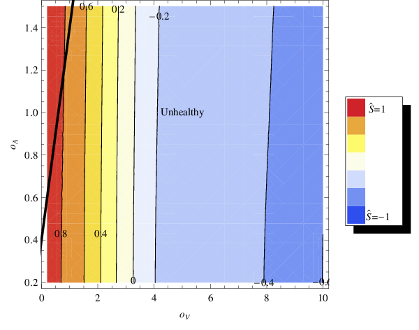
By way of illustration a survey of metrics with warp factors of the form
| (65) |
is given in fig. 3. The figure shows the parameter as a function of with the constraint from requiring that the pion be a positive-norm state added. The value of the is constrained to be positive and less than approximately 1.5 (beyond this value the axial 2-point is not defined due to the specific metric profile choice).
The chosen form of metric pre-factor can be thought of as corresponding to in the case of the earlier notation eq.(25). To see this consider the pion field with a non-zero , solve for
| (66) |
If the expression is Taylor expanded for small then one has that which implies that in the UV one is examining a bulk profile that is dual to condensate with anomalous dimension of , through the AdS/CFT dictionary.
VI.1.1 Infinite VEV Boundary Higgs
Previous authors have considered the case that the boundary breaking term is infinite. As has been shown in sec. VI.1 the theories considered that have contain a pion that is a negative-norm state.
This result has implications for the interpretation of [14]. Using the results of this sec. VI.1 one may deduce that for the (bulk) pion field to be a positive-norm state; the bulk spurion field used in [14] is a different scalar to the boundary symmetry breaking field. This can be understood by considering a higher energy theory of which [14] is the low energy effective description. If the higher theory contains a contribution to by some mechanism then this will show up in the low energy description as a fundamental contribution to .
VI.2 and Parameters
In principle, models based around eq. (8) have uncontrolled contributions to the and electroweak precision parameters [18]. Having explored the possibility of negative it is interesting to consider how these models contribute to the -order precision parameters. Restrictions on the and parameters from experiment imply an upper bound of [3]. From naïve dimensional analysis and applying the process of holographic renormalisation [18] where is the -mass and is the mass. The parameter is the renormalisation parameter that scales as . The mass of the is limited by the parameter. The value of is constrained by requiring that the theory be at large- (implying large ) and that and be within experimental bounds (implying a small or moderate ). The relationship between the bulk and boundary gauge coupling can then be used to understand whether some consistent phenomenological scenario agrees with the assumptions of the model. That is, given that the precision parameters are of acceptable values for some choice of and , is the bulk coupling perturbative. If a consistent picture is not available then one can increase the IR scale. This lowers and raise the mass. The models discussed in this work have the potential to provide scenarios where it is and that are the most constraining of the precision parameters, rather than .
Driving the IR cut-off to higher and higher values begins to imply fine tuning. For example it can be thought of as “natural” that the IR scale is of order 1 TeV because it is related to the electroweak symmetry breaking scale but increasing it greatly above such a value could be seen as questionable.
An example of this behaviour is given by,
| (67) |
Using the reasoning that allowed us to connect an “effective metric” to , this second profile, here, corresponds to slightly greater than one. In the simple case of the VEV in eq.(25), it has been shown [18] that choosing a small constrains to be below one (after saturating the bound) and thus providing an example where is the most constraining parameter.
Whilst the example given is closely linked to existing models in the literature, it serves to highlight the fact that in choosing arbitrary profiles one will produce a large number of models where and are the precision parameters that most constrain the IR cut-off of the model.
VI.3 Inclusion of Bulk Higgs Kinetic Term
In the most general case, that there is an off-diagonal bulk term, a boundary breaking term and a bulk breaking term, again one may try to play the two breaking schemes against one another and produce a negative and a healthy theory (similar to Sec. III). This study will be entirely numerical and have a number of free parameters that would be hard to control. For this reason a detailed study of this most general case is beyond the realm of the present work.
VII Conclusions
This work has investigated the possibility of a negative parameter within models of electroweak symmetry breaking formulated on a 5D slice of AdS. Attention has been given to ascertaining whether a particular scenario that gives a negative is acceptable on physical grounds.
In the simplest AdS model, which has been well-studied in the literature already, it was demonstrated that the pion field associated to the symmetry breaking is a positive-norm state if and only if is positive. In turn both of these statements are equivalent to the statement that the scaling of the condensate, , is greater than one.
To consider possibilities where is negative additional operators were added to the UV and IR boundaries, then finally also to the bulk. This indeed allowed situations where is negative. Then, within each scenario considered, the norm states of each field was considered; which limited the parameter space. This implied that it was not possible to produce a negative in a simple theory by dialing Lagrangian parameters and requiring that the theory be healthy.
One particularly interesting scenario was the addition of a bulk off-diagonal term. In principle the most constraining of the precision parameters of models which have off-diagonal contributions in the bulk can be the and parameters. This is in contrast to the usual picture that must be made to fall within bounds by dialing the IR cut-off. Instead one would need to dial the IR cut-off to make and fall within experimental bounds. On the question of whether a negative could be produced in a theory containing healthy fields it was found that this could only happen if one considered a situation with a fundamental contribution to that was negative. This would originate from a higher energy theory which the model studied in this work would be a low energy effective theory of.
In conclusion this study has not found a consistent scenario that allows for to be negative and all states to have a positive-norm, without implying a fundamental and negative contribution to originating from outside the electroweak symmetry breaking. Our survey is not totally complete, and it is possible that even higher order terms to those considered, or an ‘effective metric’ profile exists that provides a healthy theory where is negative. We have demonstrated that this would be an atypical theory and that caution should be exercised to ensure that the theory does not contain a pathology of some kind. In addition we have illustrated that frequently apparently healthy scenarios of negative can be thought of as containing a fundamental contribution to that is large and negative. In this light, it seems unlikely that a generic scenario can occur where is negative due to the contribution of electroweak symmetry breaking.
VIII Acknowledgements
This author wishes to thank M. Piai for useful discussions and interest in the project, plus comments on the manuscript. This work was funded by the Science and Technology Funding Council (STFC) research grant ST/F00706X/1.
References
- [1] M. E. Peskin and T. Takeuchi, Phys. Rev. Lett. 65, 964 (1990).
- [2] M. E. Peskin and T. Takeuchi, Phys. Rev. D46, 381 (1992).
- [3] R. Barbieri, A. Pomarol, R. Rattazzi, and A. Strumia, Nucl. Phys. B703, 127 (2004a), eprint hep-ph/0405040.
- [4] C. Csaki, C. Grojean, L. Pilo, and J. Terning, Phys. Rev. Lett. 92, 101802 (2004), eprint hep-ph/0308038.
- [5] G. Cacciapaglia, C. Csaki, C. Grojean, and J. Terning, Phys. Rev. D71, 035015 (2005), eprint hep-ph/0409126.
- [6] G. Cacciapaglia, C. Csaki, C. Grojean, and J. Terning, Phys. Rev. D70, 075014 (2004), eprint hep-ph/0401160.
- [7] S. Weinberg, Phys. Rev. D13, 974 (1976).
- [8] L. Susskind, Phys. Rev. D20, 2619 (1979).
- [9] S. Weinberg, Phys. Rev. D19, 1277 (1979).
- [10] E. Witten, Phys. Rev. Lett. 51, 2351 (1983).
- [11] B. A. Dobrescu and J. Terning, Phys. Lett. B416, 129 (1998), eprint hep-ph/9709297.
- [12] D. K. Hong and H.-U. Yee, Phys. Rev. D74, 015011 (2006), eprint hep-ph/0602177.
- [13] J. Hirn, N. Rius, and V. Sanz, Phys. Rev. D73, 085005 (2006), eprint hep-ph/0512240.
- [14] J. Hirn and V. Sanz, Phys. Rev. Lett. 97, 121803 (2006), eprint hep-ph/0606086.
- [15] J. Hirn and V. Sanz, JHEP 03, 100 (2007), eprint hep-ph/0612239.
- [16] D. D. Dietrich and C. Kouvaris, Phys. Rev. D79, 075004 (2009), eprint 0809.1324.
- [17] K. Agashe, C. Csaki, C. Grojean, and M. Reece, JHEP 12, 003 (2007), eprint 0704.1821.
- [18] M. Round, Phys. Rev. D82, 053002 (2010), eprint 1003.2933.
- [19] K. Skenderis, Class. Quant. Grav. 19, 5849 (2002), eprint hep-th/0209067.
- [20] J. M. Maldacena, Adv. Theor. Math. Phys. 2, 231 (1998), eprint hep-th/9711200.
- [21] O. Aharony, S. S. Gubser, J. M. Maldacena, H. Ooguri, and Y. Oz, Phys. Rept. 323, 183 (2000), eprint hep-th/9905111.
- [22] E. Witten, Adv. Theor. Math. Phys. 2, 253 (1998), eprint hep-th/9802150.
- [23] S. S. Gubser, I. R. Klebanov, and A. M. Polyakov, Phys. Lett. B428, 105 (1998), eprint hep-th/9802109.
- [24] L. Randall and R. Sundrum, Phys. Rev. Lett. 83, 3370 (1999), eprint hep-ph/9905221.
- [25] L. Da Rold and A. Pomarol, Nucl.Phys. B721, 79 (2005), eprint hep-ph/0501218.
- [26] J. Erlich, E. Katz, D. T. Son, and M. A. Stephanov, Phys. Rev. Lett. 95, 261602 (2005), eprint hep-ph/0501128.
- [27] M. Piai (2006), eprint hep-ph/0608241.
- [28] R. Barbieri, A. Pomarol, and R. Rattazzi, Phys. Lett. B591, 141 (2004b), eprint hep-ph/0310285.
- [29] D. D. Dietrich, F. Sannino, and K. Tuominen, Phys. Rev. D72, 055001 (2005), eprint hep-ph/0505059.
- [30] C. D. Carone, J. Erlich, and J. A. Tan, Phys. Rev. D75, 075005 (2007), eprint hep-ph/0612242.
- [31] M. Fabbrichesi, M. Piai, and L. Vecchi, Phys. Rev. D78, 045009 (2008), eprint 0804.0124.
- [32] M. Piai (2007), eprint 0704.2205.
Appendix A Solution to the Equations of Motion
Here a solution to the equations of motion for , order by order in are given. Recall the equations of motion for are
| (68) | |||||
| (69) | |||||
| (70) |
When using the choices of eq. (25) and for
| (71) | |||||
| (72) | |||||
| (73) |
where the constants are found by imposing the boundary condition.
In order to substitute into the expression for first expand in powers of .
| (74) |
Schematically, as , there is a term that diverges when giving an unbounded negative contribution to , a constant term and then higher terms that die away. Substituting the expansion of into the expression for
| (75) |
Here, the constant of integration, , has been solved for – because we are only interested in boundary conditions which lead to in the main text. The expansion in is a more compact notation for the constraint mentioned in the text that .
Alternatively one may wish to use a more general metric form. In doing so one will most likely obtain equations that require numerical solutions. An exception to this is when the bulk breaking term is switched off (or considered weak compared to another source of symmetry breaking). In the scenario that it is the boundary conditions that break the electroweak symmetry one can write down a remarkable set of equations.
| (76) | |||||
| (77) | |||||
with defined as .
Appendix B Vacuum Polarisations
By solving the bulk equations of motion eq.(14) for the choice of eq. (25) and substituting into the definition of the vacuum polarisation one obtains the unrenormalised expression for . Then the counterterm is dialed to give
| (78) |
for the Euler-Mascheroni number and Bessel functions. In order to produce this expression a normalisation of has been chosen by choosing at .
The expression for allows the spectrum to be read off. There is a massless photon and a tower of heavier states with the same quantum numbers as the Standard Model photon. The first such state will be referred to as the in analogy with QCD and has a mass dependent upon . The mass for particular values of can be given as
| (79) |
To obtain the axial vacuum polarisation, , the expressions for are used. The counterterm removes the log-divergence originating from . The result for is
| (80) |
Assume that the first zero of the vacuum polarisation can be well approximated by the ratio of the first two terms in the expansion of . Provided that and the mass is approximately
| (81) |