Oscillating Bianchi IX Universe in Hořava-Lifshitz Gravity
Abstract
We study a vacuum Bianchi IX universe in the context of Hořava-Lifshitz (HL) gravity. In particular, we focus on the classical dynamics of the universe and analyze how anisotropy changes the history of the universe. For small anisotropy, we find an oscillating universe as well as a bounce universe just as the case of the Friedmann-Lemaitre-Robertson-Walker (FLRW) spacetime. However, if the initial anisotropy is large, we find the universe which ends up with a big crunch after oscillations if a cosmological constant is zero or negative. For , we find a variety of histories of the universe, that is de Sitter expanding universe after oscillations in addition to the oscillating solution and the previous big crunch solution. This fate of the universe shows sensitive dependence of initial conditions, which is one of the typical properties of a chaotic system. If the initial anisotropy is near the upper bound, we find the universe starting from a big bang and ending up with a big crunch for , while de Sitter expanding universe starting from a big bang for .
pacs
04.60.-m, 98.80.Cq, 98.80.-kI Introduction
Since the advent of the big bang theory, the initial singularity problem is of prime importance in the field of cosmology. As shown by Hawking and Penrose[1], general relativity (GR) predicts a spacetime singularity if a certain condition is satisfied. Their singularity theorem concludes that our universe must have an initial singularity. However, once a singularity is formed, general relativity becomes no longer valid. It must be replaced by more fundamental gravity theory. Even in the framework of an inflationary scenario which resolves many difficulties in the early universe based on the big bang theory, the initial singularity cannot be avoided. New gravitational theory may be required to describe the beginning of the universe.
Many researchers attempt to resolve this singularity problem in the context of generalization or extension of general relativity[2]. However, no success has been achieved yet. Superstring theory, which is one of the most promising candidates for unified theory of fundamental interactions, may solve it, but so far it has not been completed yet and is not so far able to describe any realistic strong gravitational phenomena. Loop quantum gravity theory may resolve the problem of a big bang singularity via loop quantum cosmology[3]. However it is still unclear how to describe time evolution of quantum spacetime in loop quantum gravity because of the lack of “time” variable.
Among attempts to construct a complete quantum gravitational theory, Hořava-Lifshitz (HL) gravity has been attracted much interest as a candidate for such a theory over the past years. HL gravity is characterized by its power-counting renormalizablity, which is brought about by a Lifshitz-like anisotropic scaling as , with the dynamical critical exponent in the ultra-violet (UV) limit [4]. In order to recover general relativity (or the Lorentz invariance) in our world, one expects that the constant converges to unity in the infrared (IR) limit in the renormalization flow. Although it has been argued that there exist some fundamental problems in HL gravity [5, 6, 8, 11, 13, 7, 9, 10, 12, 14, 15, 16], some extensions are proposed to remedy these difficulties[19, 10, 17, 18]. It is intriguing issue whether or not HL gravity can be a complete theory of quantum gravity.
There are a number of works on cosmology in HL gravity [7, 34, 20, 22, 23, 24, 25, 26, 29, 31, 21, 27, 28, 30, 32, 37, 39, 40, 41, 43, 44, 46, 35, 38, 36, 47, 48, 49, 50, 51, 33, 52, 53, 42, 45]. As pointed out by earlier works, a big bang initial singularity may be avoided in the framework of HL cosmology due to the higher order terms in the spatial curvature in the action [38]. In this context, many researchers have studied the dynamics of the Friedmann-Lemaitre-Robertson-Walker (FLRW) universe in HL gravity [37, 39, 40, 41, 43, 44, 46, 35, 38, 36, 47, 48, 49, 50, 51, 42, 45]. In isotropic and homogeneous spacetime, higher curvature terms with arbitrary coupling constants mimic various types of matter with arbitrary sign of energy densities. The and scaling terms give “dark radiation” and “dark stiff-matter”, respectively. Although “dark radiation” terms in the models with the detailed balance condition can avoid the initial singularity, such terms may become irrelevant to the dynamics when we include relativistic matter fields, which may scale as in the UV limit and behave as a stiff matter[21].
In our previous paper [47], we have studied the dynamics of vacuum FLRW spacetime in generalized HL gravity model without the detailed balance condition and shown that “dark stiff-matter” can avoid the initial singularity of the universe. Even if we include relativistic matter fields, when the contribution of “dark stiff-matter” is dominant, the singularity is avoided and an oscillating spacetime or a bounce universe is obtained.
Although we have shown a singularity avoidance in HL cosmology, the following question may arise: Is this singularity avoidance generic? Is such a non-singular spacetime stable against anisotropic and/or inhomogeneous perturbations? In order to answer for these questions, we have to study more generic spacetime than the FLRW universe.
The initial state of the universe could be anisotropic and/or inhomogeneous. Before the singularity theorem, some people believed that the big bang singularity appears because of its high symmetry and it may be resolved if one studies anisotropic and/or inhomogeneous spacetime. Then they analyzed anisotropic Bianchi-type universes and their generalization. Although they found some interesting behaviours near the singularity such as chaos in Bianchi IX spacetime [54, 55, 56, 57], they could not succeed the singularity avoidance. It is simply because the singularity theorem does not allow a singularity avoidance in GR. The situation becomes worse if we consider anisotropy and/or inhomogeneity. Even in the effective gravity model derived from superstring, which shows a singularity avoidance, with such a property[58, 59], once we include anisotropy and/or inhomogeneity, the property of such a singularity avoidance may be spoiled[60].
Therefore it is important to study whether or not non-singular universes in the present HL cosmology still exist with anisotropy and/or inhomogeneity. In the present paper, we shall investigate the possibility of the singularity avoidance in homogeneous but anisotropic Bianchi IX universe. Since we are interested in a singularity avoidance, we focus on an oscillating universe and analyze how anisotropy changes the history of the universe. We will not study the chaotic behaviour in detail, which may appear near the big bang singularity, although it is one of the most popular and important properties in the Bianchi IX spacetime and was discussed analytically in [52, 53]. As we will show later, however, some property of non-integrable system, i.e., sensitive dependence on initial conditions may be found in the fate of the universe in the present analysis as well.
The paper is organized as follows. After a short overview of HL gravity, we present the basic equations for the vacuum Bianchi IX universe in HL gravity in Sec.II. In Sec.III, we study the stability of the closed FLRW universe against small anisotropic perturbations. In Sec.IV we analyze Bianchi IX universe numerically and show a variety of histories of the universe, depending on initial anisotropy. Summary and remarks follow in Sec.V. In Appendix, we also analyze a bounce universe with anisotropy as an another type of non-singular solution.
II Bianchi IX universe in Hořava-Lifshitz gravity
First we introduce our Lagrangian of HL gravity, by which we will discuss the Bianchi IX universe. The basic variables in HL gravity are the lapse function, , the shift vector, , and the spatial metric, . These variables are subject to the action [4, 19]
| (1) |
where (: the Planck mass) and the kinetic term is given by
| (2) |
with
| (3) | |||
| (4) |
being the extrinsic curvature and its trace. The potential term will be defined shortly. In GR we have , only for which the kinetic term is invariant under general coordinate transformations. In HL gravity, however, Lorentz symmetry is broken in exchange for renormalizability and the theory is invariant under the foliation-preserving diffeomorphism transformations,
| (5) |
As implied by the symmetry (5), it is most natural to consider the projectable version of HL gravity, for which the lapse function depends only on : [4]. Since the Hamiltonian constraint is derived from the variation with respect to the lapse function, in the projectable version of the theory, the resultant constraint equation is not imposed locally at each point in space, but rather is an integration over the whole space. In the cosmological setting, the projectability condition results in an additional dust-like component in the Friedmann equation [7].
The most generic form of the potential is given by [19]
| (6) | |||||
where is a cosmological constant, and are the Ricci and scalar curvatures of the 3-metric , respectively, and ’s () are the dimensionless coupling constants. By a suitable rescaling of time we set . We also adopt the unit of () throughout the paper.
Let us consider a Bianchi IX spacetime, which metric is written as
| (7) |
where the invariant basis is given by
| (8) |
A typical scale of length of the universe is given by , which reduces to the usual scale factor in the case of the FLRW universe. We shall call it a scale factor in Bianchi IX model as well. The traceless tensor measures the anisotropy of the universe. The spacelike sections of the Bianchi IX is isomorphic to a three-sphere , and a closed FLRW model is a special case of the above metric in the isotropic limit ().
For a vacuum spacetime, without loss of generality, we can assume that is diagonalized as
| (9) |
The basic equations describing the dynamics of Bianchi IX spacetime in HL gravity are now given by the followings:
| (10) |
| (11) |
| (12) |
where is the Hubble expansion parameter, i.e., the volume expansion rate is given by . The constant arises from the projectability condition and it could be “dark matter” [7], but here we assume just for simplicity.
The potential , which depends on as well as , is defined by
| (13) |
where
| (14) | |||||
| (15) | |||||
| (16) | |||||
| (17) |
Although the similar potential was found in [53], we extend it to the case without the detailed balance condition.
III Linear Perturbations of the FLRW universe
In this section, we shall analyze the present system with small anisotropies by linear perturbations of the FLRW universe. We discuss the stability of the oscillating FLRW universe and present a new type of non-singular solutions.
III.1 Oscillating Closed FLRW Universe
First we summarize the result of the closed FLRW spacetime, which metric is given by
| (18) |
We find the Friedmann equation as
| (19) |
where
| (20) |
The coefficients and are defined by
| (21) |

(a) for

(b) for

(c) for
The conditions for an oscillating FLRW universe to exist
were already given in [47],
which are summarized as follows:
(a)
| (22) |
(b)
(c)
| (26) |
where , and is defined by
| (27) |
with being the sign of .
We show the typical shapes of the potential in Fig. 1 for the coupling parameters which we use in our numerical analysis. For an oscillating universe, is bounded in a finite range as .
III.2 Linear Stability of the FLRW Universe
As we mentioned in Introduction, a non-singular FLRW universe such as an oscillating universe should be stable against anisotropic perturbations. Otherwise such a spacetime may not be realized in the history of the universe. Hence, in this subsection we study stability of the FLRW universe against linear anisotropic perturbations.
When the anisotropic part of metric vanishes,i.e., , Eq. (10) reduces to the usual Friedmann equation (19) for a closed universe. For the stability analysis, we expand the potential around the FLRW universe with to second order of , so that
| (28) | |||||
| (29) | |||||
| (30) | |||||
| (31) |
The total potential is thus approximated by
| (32) |
where
| (33) | |||||
| (34) | |||||
In order to ensure that the FLRW universe is stable against small anisotropic perturbations, we impose the condition . The sufficient condition for stability is obtained if all coefficients in are positive because is positive, i.e.,
| (35) | |||||
| (36) | |||||
The necessary and sufficient conditions for stability are obtained by taking into account the dynamics of the background FLRW universe, i.e., the time evolution of a scale factor . We will cover a wider range of the coupling parameters than the above. To show the explicit necessary and sufficient conditions, just for simplicity, we restrict our analysis to the case with , i.e., the parity-conserved theory. In this case, can be recast in
| (37) | |||||
The stability condition is such that for (the range in which the oscillation occurs). When , and are given explicitly by
| (38) |
We thus find that either of the following three conditions must be satisfied to ensure the stability:
| (39) |
or
| (40) |
or
The above inequalities give the necessary and sufficient conditions for a stable oscillating FLRW universe in the case of and . Since in more general cases with and/or , the necessary and sufficient conditions could be obtained straightforwardly but would be much more involved, we dare not list the full conditions in the present paper. It may be sufficient to demonstrate that the stability range of coupling parameters exists without any fine tuning.
III.3 Perturbation around a static universe
Next we provide a simple and illustrative example in which even small anisotropies can bring in a possibly interesting cosmological dynamics.
Let us consider the case with , , and , so that we find a static FLRW universe with the constant scale factor . We then add small anisotropic perturbations to this static background. The basic equations governing the system are given by
| (42) | |||||
| (43) |
where
| (44) |
Integrating Eqs. (42) and (43), we find conserved anisotropic energies defined by
| (45) |
Using the constants we obtain the equation for the scale factor as
This equation gives an oscillating solution for with the frequency
| (47) |
Similarly, also oscillate with the frequencies
| (48) |
The ratio of two frequencies and is given by
Those frequencies give the typical values of the present oscillating system. They and their ratio are fixed only by the coupling parameters (’s) because and are given by them.
The above perturbative analysis around a static universe shows that an oscillating solution newly appears in the presence of the small anisotropies . As the argument here is based on perturbations , one may wonder whether or not there exist similar oscillating solutions with large anisotropies. We are going to perform numerical calculations to explore the anisotropic cosmological dynamics arising from more general setups beyond perturbations.
IV Anisotropic oscillating universe in Hořava-Lifshitz gravity
In the previous section, we have shown that an oscillating FLRW solution in HL gravity is stable against small anisotropies, , for a wide range of the coupling parameters. We now proceed to investigate the rich variety of the dynamics of oscillating universes in the context of Bianchi IX spacetime, extending the analysis to the case with large anisotropies.
If are not small, the previous perturbative approach is no longer valid. To extend the analysis to include the case with large anisotropies, we employ a numerical approach and solve the governing equations without any perturbative expansion. With this, we intend to uncover the rich variety of anisotropic cosmology and clarify the resultant fate of the universe.
We have already given the basic equations for the Bianchi IX universe in HL gravity. It will be convenient to rewrite the equations as
| (49) | |||
| (50) | |||
| (51) | |||
| (52) |
where
| (53) |
is the shear tensor of a timelike normal vector perpendicular to the homogeneous three-space, and is its magnitude. It may be convenient to introduce the dimensionless shear by
| (54) |
which measure the relative anisotropies to the expansion rate . We also introduce the phase variable defined by
| (55) |
which parameterizes the direction of the anisotropic expansion.
We have the five first-order evolution equations for , and , i.e., Eqs. (50), (51)and (52), supplemented with one constraint (49). We have to set up the initial values for five of the six variables, and . The other one is fixed by the constraint equation. Since we are interested in how the cosmological dynamics is altered by the introduction of anisotropies, we start with the isotropic oscillating universe by setting to vanish and to be a local minimum of , with arbitrary shear ( and ) at the initial moment. So we shall give the initial data for and , and then determine (or ) by the constraint (49).
Without any loss of generality, we can analyze only the range of because of the discrete symmetry modulo of the potential . Since is negative (therefore is positive) for the oscillating FLRW universe, the possible range of initial shear is limited from Eq.(50) as
| (56) |
As we discussed in the previous section, the FLRW universe is stable against small anisotropic perturbations if defined by Eq. (37) is positive. However one may suspect that it becomes unstable when anisotropy is large. For stability against large anisotropy, we have one natural indicator, which is the potential . If the potential is unbounded from below for large , we expect that if initially large will diverge in time and the universe evolves into a singularity.
From Eq. (14), we find that the potential is bounded from below, if and only if one of the following conditions is satisfied:
| (57) | |||||
| (58) | |||||
| (59) | |||||
| (60) |
We then classify the potential into four types: SS, US, SU, and UU, where the first S (stable) or U (unstable) denotes the stability against small perturbations around FLRW spacetime, while the second S (stable) or U (unstable) corresponds to the stability against large anisotropies. Since a cosmological constant will also change the fate of the universe, we shall discuss eight types of cosmological models; Models I-SS, I-SU, I-US, I-UU, II-SS, II-SU, II-US, and II-UU, depending on the sign of (I for and II for ) and the potential types.
| Model | Figures | ||||||
|---|---|---|---|---|---|---|---|
| I-SS | 0 | SS | 1 | 0 | Figs. 2-9 | ||
| I-SU | 0 | SU | 1 | Figs. 10-12 | |||
| II-SS | SS | 1 | 0 | Figs. 13-17 |
Note that a singularity, of course, may appear even for small anisotropies because the Bianchi IX spacetime includes a closed FLRW model.
We have performed numerical calculations for all possible models and various initial data. Now we show our numerical results for each model. We find several types of fates of the universe depending on the magnitude of anisotropy, which we shall describe one by one.
In Table 1, we list up the values of parameters for which we present the figures in this paper.
IV.1 Model I-SS ( and Type-SS potential)
First we discuss Model I-SS, in which and the potential is the SS type. Since the universe is closed, there are two fates: an eternal oscillation or a big crunch. Depending on the strength of initial anisotropy, we find the following three types of histories of the universe.
- (A)
Anisotropic oscillation : (small anisotropy)

(a) the time evolution of scale factor

(b) the phase space of
Figure 2: The time evolution of non-singular oscillating universe. The solid blue line and dashed red line represent Bianchi IX universe and FLRW universe with the same initial , respectively. We show the scale factor in (a) and the orbit of in the phase space in (b), respectively. We set the initial values as , , and . 
(a) the orbit of ()

(b) the evolution of the shear
Figure 3: The orbit of anisotropy and the time evolution of the shear of the oscillating universe given in Fig. 2. Since we have an oscillating universe for the FLRW spacetime, we find an eternally oscillating non-singular solution if is sufficiently small (). A typical example is given in Fig. 2. The scale factor is regularly oscillating with time just as the FLRW solution with the same initial scale factor , which is shown by the dotted red curves as a reference.
This oscillating solution shows only small deviation from the isotropic FLRW universe. The scale factor (and then the volume) oscillates very regularly. Its orbit in the phase space shows an ellipse (a cross section of a torus) (see Fig. 2(b)). The radius is slightly larger than that of the FLRW universe because of the existence of shear (see Eq. (49))
The orbit of the anisotropy is depicted in Fig. 3(a). The anisotropic variables are trapped around the origin of -space by the potential wall. It looks complicated but definitely periodic. The shear is also regularly oscillating as shown in Fig. 3(b), but the oscillation period is much shorter than that of the scale factor . The oscillation amplitude of the shear is then modulated by -oscillation. We can estimate those oscillation frequencies from the result in §III.3. Using the coupling parameters of the present model (see Table 1), we find and from Eqs. (47) and (48), which are almost the same as the frequencies in Figs 2(a) and 3(b).
The resultant universe is regarded as an isotropic spacetime with small anisotropic perturbations. The anisotropic oscillation may continue eternally.
- (B)
Big crunch after oscillations : (large anisotropy)
If is large as , an initially oscillating universe eventually collapses into a big crunch () after many oscillations because of increase of the anisotropy. A typical example of such a singular universe is shown in Fig. 4.
(a) scale factor

(b) phase space
Figure 4: The time evolution of the unstable oscillating Bianchi IX universe. The dashed red line shows the FLRW spacetime. We set the initial values as , , and . The oscillation period is almost the same as that in Fig. 2(a). As shown in Fig. 4 (b), the orbit of the scale factor in the phase space is initially almost an ellipse (a cross section of a torus), but its “radius” gradually increases because of the increasing anisotropy, and finally evolves into a big crunch singularity ().

(a) the orbit of

(b) the evolution of shear
Figure 5: The time evolution of the shear of the unstable oscillating universe given in Fig. 4. The behaviour of anisotropy is shown in Fig. 5(a), which shows that the orbit of is trapped and reflected many times by the potential wall. The shear is initially oscillating and eventually diverges at a big crunch as shown in Fig. 5(b). Before this divergence, we can see the increase of , which leads the leave from the oscillating phase. Then the universe eventually evolves into a singularity with finite values of . Note that the relative shear is finite at the end, which means that the shear is not responsible for the singularity.
In Fig. 6, we show the curvature invariant
(61) which really diverges at a big crunch singularity. The universe evolves into a big crunch after many oscillations.

Figure 6: The time evolution of the extrinsic curvature square of the unstable oscillating universe given in Fig. 4. For the Bianchi IX universe (solid blue line), oscillates in the beginning, but it eventually diverges at the end of the evolution, while it just oscillates periodically for the FLRW universe. - (C)
From big bang to big crunch :
(near maximally large anisotropy)
Another type of singular solution is found for the extremely large initial anisotropy (). In the case of the closed FLRW universe in GR, the spacetime starts from a big bang and ends up with a big crunch. Bianchi IX universe in GR also evolves from zero volume (a big bang) to zero volume (a big crunch) through a finite maximum volume. Hence even for the case with the oscillating FLRW universe, if we add a sufficiently large anisotropy, we may expect such a non-oscillating simple evolution.We show one example. As shown in Fig. 7, the scale factor evolves from an initial finite value to a singularity (), which is called a big crunch. If we calculate the time reversal one from the same initial data, we will find a singularity (), which is called a big bang. As a result, this universe starts from a big bang and ends up with a big crunch. There is no oscillation in the evolution of just as the closed FLRW universe in GR.

Figure 7: The time evolution of the scale factor of the Bianchi IX universe with the potential given in Fig. 6 is shown by the solid blue line. The dashed red line represents the oscillating FLRW universe. We set set the initial values as , , and . As for the anisotropy, as shown in Fig. 8, the orbit of is oscillating around the origin and reflecting at the potential wall until formation of a singularity. is finite even at a big crunch.

(a) anisotropy ()

(b) shear square
Figure 8: (a) The orbit of anisotropy () and (b) the time evolution of the shear square of the universe given in Fig. 7. The shear is also oscillating, but the frequency is not so regular compared with the previous two cases (A) and (B).
The shear diverges at a big crunch (), which is really singular because the extrinsic curvature square also diverges there as shown in Fig. 9. The behaviour of is very similar to that of the shear square. However the relative shear does not diverge at a big crunch, which means that the singularity is similar to that of the FLRW universe. The shear does not dominate in the dynamics (Compare it with next example (C)′).

Figure 9: The time evolution of the extrinsic curvature square for the solution shown in Fig. 7. The solid blue line and dashed red line represent Bianchi IX universe and FLRW universe, respectively. It diverges at the end of evolution, which is a singularity. In the case of a negative cosmological constant (), we also find the similar behaviour of the universe, although there is a quantitative difference.
IV.2 Model I-SU ( and Type-SU potential)
When the potential is unbounded from below, the universe may be unstable against large anisotropic perturbations (see Fig. 10).
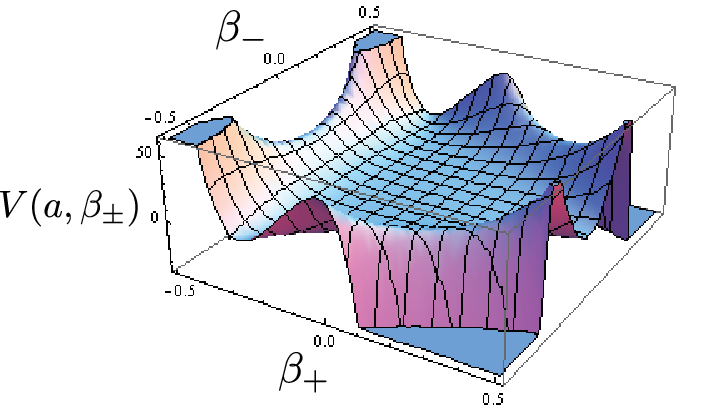
Figure 10: The unstable potential against large anisotropic perturbations is shown for . We also find three types of histories of the universe as (A), (B), and (C) in Model I-SS. The difference from Model I-SS appears when anisotropy gets large. That is, the anisotropy diverges when a singularity appears. We show one example with near maximally large initial anisotropy.
- (C)′
From big bang to big crunch :
(near maximally large anisotropy)
In this case, just as the history (C) of Model I-SS, the Bianchi IX universe expands from zero volume to zero volume without oscillation (Fig. 11).
Figure 11: The time evolution of the scale factor of the Bianchi IX universe is shown by the solid blue line. The dashed red line represents the oscillating FLRW universe. We set set the initial values as , , and . 
(a) anisotropy ()

(b) shear square
Figure 12: (a) The orbit of anisotropy () and (b) the time evolution of the shear of the universe given in Fig. 11. . The difference appears in the behaviour of , which diverges at a big crunch. The orbit of initially oscillates around the origin and reflects on the potential wall, but it eventually evolves to infinity over the potential hill because the potential is not bounded from below (see Fig. 12(a)). We also show the time evolution of the shear , which diverges at the end of the universe. The extrinsic curvature square also diverges there, which means it is really a singularity.

Figure 13: The time evolution of the relative shear square of the universe shown in Fig. 11 This singularity is different from one appeared in the history (B) or (C). To show it, we depict the time evolution of the relative shear , which diverges at a big crunch. It means that the shear becomes dominant at the end. The increase of the anisotropic shear is responsible for the formation of a singularity. Note that diverges also in the middle of the evolution but its divergence appears because of .
At a big bang, which appears in the time reversal one, we suspect that the shear diverges but is finite just as the beginning of Bianchi IX universe in GR.
IV.3 Model II-SS ( and Type-SS potential)
Next we discuss the case of . In this case, we find another fate of the universe, which is an exponentially expanding universe by a positive cosmological constant.
If the effect of anisotropy is smaller than the contribution of a cosmological constant, the universe will be isotropized. The asymptotic equation for is given by
| (62) |
if we neglect the anisotropic terms in Eq. (11), finding an exponentially expanding FLRW spacetime, i.e., de Sitter spacetime;
| (63) |
with
| (64) |
Along with the cosmic expansion the potential is flattened to be negligible in the evolution equation for the anisotropy because increases rapidly, so that we find
| (65) |
from Eq. (43). This implies that asymptotically due to the Hubble friction. Since the shear decreases to zero, the universe becomes locally isotropic, i.e., locally de Sitter spacetime. Note that this does not mean that it is globally de Sitter spacetime because the asymptotic values of do not vanish. However the spacetime is exponentially expanding, and the observable region such as a horizon scale becomes effectively isotropic. Hence we shall still call this asymptotic spacetime de Sitter universe.
As a result, we have three fates of the universe in the case with : oscillating universe, a big crunch, and de Sitter expanding universe. We then find five types of histories of the universe: two new types with asymptotically de Sitter universe in addition to the previous three types (A), (B) and (C) discussed in IV.1.
Two new types are the similar to the histories (B) and (C), but different from those in their final states, i.e., (D) de Sitter expansion after oscillation, and (E) de Sitter expansion from a big bang.
For small anisotropy (), we find the oscillating universe (A) . While for the large anisotropy (), the universe is either Type (B) or Type (D). When the initial anisotropy is extremely large enough, i.e., , Type (C) or Type (E) is obtained. We shall describe new types (D) and (E) below.
- (D)
de Sitter expansion after oscillation :
(large anisotropy)We show one example in Fig. 14.

Figure 14: The time evolution of the scale factor of the universe with . The solid blue line and dashed red line represent Bianchi IX universe and FLRW universe, respectively. We choose the coupling constants as , , ,, , and , and set the initial values as , , and . 
(a)

(b)

(c)
Figure 15: The time evolution of the shear square and anisotropies of the universe shown in Fig. 14. The shear oscillates initially, but the universe suddenly leaves the oscillating phase to de Sitter expanding phase, which drops the shear to zero rapidly. The initially oscillating finally settles to finite values after small bump. If is as large as , an initially oscillating universe eventually evolves into an exponentially expanding de Sitter universe because of a cosmological constant.
The initially oscillating universe leaves the oscillation phase when the anisotropy increases beyond some critical value. We also show the evolution of the shear in Fig.15. We find that it is oscillating regularly for two-third of the whole period, but eventually increases. Then the universe leaves the oscillating phase and evolves into de Sitter phase. Because of rapid expansion of the universe, the shear vanishes soon [61].
We also show the time evolution of the anisotropy () in Fig. 15(b),(c). The initially oscillating anisotropy increases as a burst and then decreases to a small finite constant.
How the universe choose its fate ((B) or (D)) is as follows: If the spacetime is expanding when it leaves from the oscillating phase, it evolves into de Sitter phase (D), while if it is contracting, it collapses to a big crunch (B).
- (E)
de Sitter expansion from big bang :
(near maximally large anisotropy)
If is close to the maximum value () and the universe is initially expanding (), the spacetime evolves into de Sitter phase without oscillation. The large anisotropy makes a jump from the oscillating phase to de Sitter phase in the beginning. The anisotropy drops quite rapidly because of the exponential expansion as shown in Fig. 17.
Figure 16: The time evolution of the scale factor of the universe with and Type-SU potential. The universe starts from a big bang and evolves into de Sitter spacetime. The dashed red line represents the oscillating FLRW universe as reference. On the other hand, if the universe is initially contracting (), the spacetime is classified into Type (C), i.e., from a big bang, which appears in the time reversal one, to a big crunch without oscillation.

Figure 17: The time evolution of the shear of the universe shown in Fig. 16. Initially oscillating shears drops to zero after de Sitter expansion starts. IV.4 Model II-SU ( and Type-SU potential)
In this case, we also find the similar histories of the universe to Types (A), (B), (C), (D) and (E), depending on initial anisotropies. The differences between Models II-SS and II-SU are qualitatively the same as those between Models I-SS and I-SU. Only one difference from Model I is that there exists de Sitter phase as the fate of the universe because of a positive cosmological constant.
IV.5 Models with the unstable potential against small perturbations around FLRW spacetime
In the previous four subsections, we discuss the cosmological models with the stable potential against small perturbations around FLRW spacetime. When the potential is unstable against small perturbations around FLRW spacetime, we also find qualitatively similar results. The main difference is that oscillations around the FLRW spacetime never happen. Even if the universe starts from near FLRW spacetime, it evolves into spacetime with large anisotropy because the FLRW spacetime is unstable. As a result, in the case of Type-UU potential, the universe collapses to a singularity for Model I-UU. No oscillating phase is found. If , i.e., for Model II-UU, some universe collapses to a singularity without oscillations, and the other one evolves into de Sitter expanding universe, depending on initial conditions.
IV.6 Dependence of anisotropy on the date of the universe
In Table 2, we summarize the fate of the universe. We assume the coupling parameters by which there exists an oscillating FLRW universe. For Models I-SS and II-SS, we find an oscillating FLRW universe with anisotropy in the case of small initial anisotropy. When we increase the strength of anisotropy, the spacetime leaves the initially oscillating phase and eventually evolves into a singularity or de Sitter spacetime. If the initial anisotropy is near the maximum value, the oscillating phase disappears and a simply expanding and contracting universe is found just as a closed universe in GR for . When , an initially expanding universe evolves into de Sitter spacetime, while an initially contracting universe evolves into a big crunch.
| Model | cosmological | potential | |||||
|---|---|---|---|---|---|---|---|
| constant | small | large | near maximally large | ||||
| I-SS | SS | (A) OSC | (B) OSCSING | (C) SING | |||
| I-US | US | (A) OSC | (B) OSCSING | (C) SING | |||
| I-SU | SU | (A) OSC | (C)′ SING | ||||
| I-UU | UU | (C)′ SING | |||||
| II-SS | SS | (A) OSC | (B)(D) OSCdeS/SING | (E) deS [(C) SING] | |||
| II-US | US | (A) OSC | (B)(D) OSCdeS/SING | (E) deS [(C) SING] | |||
| II-SU | SU | (A) OSC | (E)′ deS [(C)′ SING] | ||||
| II-UU | UU | (E)′ deS [(C)′ SING] |
For Models I-US and II-US, the histories of the universes are similar to those in Models I-SS and II-US, respectively, although deviation from isotropy becomes large even for initially small anisotropy.
In the cases of Models I-SU and II-SU, unless an initial anisotropy is small, an initially expanding universe turns to contract and collapses into a big crunch for , while it evolves into de Sitter spacetime for . This singularity at a big crunch is different from that in Models I-SS,-US, and II-SS, US. The anisotropy for the present model diverges, while that for the other cases is finite even at a singularity.
Models I-UU and II-UU are not so interesting. There is no oscillating phase. If , the spacetime is simply a spacetime evolving from a big bang to a big crunch. For , the initially expanding universe evolves into de Sitter spacetime, while the contracting one collapses into a singularity.

(a)

(b)
One may wonder whether the initial anisotropy classifies the fate of the universe. Are there any critical values of the initial anisotropies for their transitions in Table 2 ? We understand naively that such a transition occurs as the anisotropy increases.
We find there exists a critical value for the transition (B) to (C) or (D) to (E), which is about . For the transition from (A) to (B) (or (D)), it is not so clear whether there exists a critical value of or not. If is sufficiently small, we find the history (A), while when it is large, we find the history (B) or (D). However, because we analyze the system numerically, we are not sure whether the model with small anisotropy oscillates forever or will turn to collapse long after. If the latter case is true, the case with small anisotropy is classified into the history (B) or (D). So there may not be exactly the history (A) except for the exact FLRW spacetime.
More interesting fact is found in the history (B)(D) for . In order to study how the fate of the universe depends on the initial data, we solve the basic equations in Model II-SS assuming various initial values of anisotropy ( and ). We summarize the results in Fig. 18. As we see from Fig. 18, the spacetime with starting from near maximum anisotropy evolves into de Sitter universe (the history (E)), while it collapses into a singularity if (the history (C)). For small , we find an oscillating universe (the history (A)). If is between the above two cases, however, the fate of the universe is not so simple. The history of such a universe is classified either (B) OSCSING1 or (D) OSCdeS. However such a history does not shift monotonically from (B) to (D) as the initial anisotropy increases. How the universe choose its fate ((B) or (D)) as follows: If the spacetime is expanding when it leaves from the oscillating phase, it evolves into de Sitter phase (D), while if it is contracting, it collapses to a big crunch (B). As a result, the fate of the universe is sensitively dependent on initial conditions. If one changes the initial conditions, the fate changes drastically. It is because the present system is non-integrable. Such a property is found in a dynamical system with chaos. Since our model is Bianchi IX, which shows chaotic behaviour near singularity in GR[55, 56, 57], we understand why we find such a complicated basin structure of the fate in Fig. 18, which can be fractal[57].
V Summary and remarks
We have explored a singularity avoidance in a vacuum Bianchi IX universe in HL gravity. We have studied an oscillating cosmological solution with anisotropy. In the case of small anisotropy (), we find an analytical solution and show the stability condition of the FLRW universe against anisotropic perturbations. We have also solved the basic equations numerically and discussed the possible history of the universe. We classify our models into eight types I-SS,-SU,-US,-UU, and II-SS, -SU,-US,-UU, depending on the sign of a cosmological constant and the types of the potential . We find five types of the histories of the universe: (A) an oscillating universe with anisotropy, (B) a big crunch after oscillations, (C) from a big bang to a big crunch, (D) de Sitter expansion after oscillations and (E) from a big bang to de Sitter expansion, as summarized in Table 2.
The stable oscillating universe (A) is found if initial anisotropy is small in the case that the coupling parameters (s) satisfy the stability condition. When initial anisotropy is large, the oscillating universe evolves into a singular big crunch (B) for . In the case of , if the initial anisotropy is large but not close to the maximum value, we find two histories (B) and (D). Which history is realized does not depend monotonically on the initial shear , but the present system shows sensitive dependence of initial conditions just as one of the typical properties of chaos. The anisotropic bounce universe is also obtained for the model satisfied the stability condition if initial anisotropy is small.
Since we adopt the unit of , the oscillation period and oscillation amplitude are the Planck scale, unless the coupling constants are unnaturally large. Hence in order to obtain a macroscopic universe, we need a positive cosmological constant , which provides us a de Sitter expanding phase.
In a more realistic situation, this cosmological constant should be replaced by a potential of an inflaton scalar field . Reheating after inflation may give an initial state of a macroscopic big bang universe.
When we include a scalar field, however, we have to take into account modification of a scalar field action in the UV limit similar to HL gravity action. The action may be given by
| (66) |
where
| (67) |
with being a typical mass scale and s () being dimensionless constants. For this action with HL gravity action (1), the basic equations for a Bianchi IX cosmological model are given by
| (68) | |||
| (69) | |||
| (70) | |||
| (71) |
Although the action (66) contains higher spatial derivatives, there exists no difference from the conventional canonical kinetic term of a scalar field for a homogeneous spacetime. We expect a usual inflationary scenario once de Sitter exponential expansion starts. There exists reheating after slow-roll inflation, finding a big bang universe.
If we have an oscillating phase before inflation, we may expect one interesting effect, which is modification of primordial perturbations. We should stress that a classical transition from an oscillating phase to an inflationary stage never happens in the FLRW model (See our discussion in [47] for quantum transition). So anisotropy may be important in the pre-inflationary oscillating phase. As a result, we may find large non-Gaussian density perturbations. To confirm our scenario, we should explore the dynamics of a scalar field in the pre-inflationary era because in an inflationary model may be fluctuated by the oscillating scale factor in the pre-inflationary era while is a constant in our present analysis.
Another interesting possibility is anisotropic inflation, which is discussed in the model with higher curvature terms[62] or with a vector field[63]. It may leave distinguishable imprints on the primordial perturbations.
Acknowledgements.
TK would like to thank RESCEU, the University of Tokyo, where a large part of this work was completed. This work was supported in part by JSPS Grant-in-Aid for Research Activity Start-up No. 22840011 (TK), by JSPS Grant-in-Aids for Scientific Research Fund No.22540291 (KM) and by JSPS under the Japan-Russia Research Cooperative Program (KM).Appendix A Anisotropic bounce universe in Hořava-Lifshitz gravity
In the text, we have considered oscillating universes as a possible way to avoid an initial singularity. In this appendix, we study another way to singularity avoidance, i.e., a bounce solution [47]. For a closed FLRW universe, a bounce solution exists only only in the case of . As a result, a bounce solution with anisotropy is also found only for the case of .
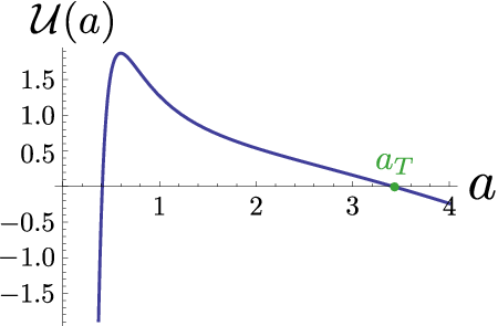
We classify bounce solutions into two classes according to the shape of the potential . The first class is such that , which we call Type A, and the other is such that , which we call Type B. We show two typical potentials in Fig. 19.
(a) Type A
(b) Type B
For Type-A potential, in addition to a bounce solution, we find a FLRW spacetime starting from a big bang and collapsing to a big crunch, while for Type-B potential, we have an oscillating FLRW solution as well as a bounce spacetime. This difference gives rise to different fates of anisotropic Bianchi IX universe as we will show later.
When initial anisotropy is small, it is easy to find anisotropic bounce solutions because anisotropy can be treated as perturbations around the isotropic closed FLRW universe. In order for this type of stable solutions to exist, the condition () must be satisfied. The sufficient condition for stability is the same as Eq. (36).
If the stability condition is not satisfied, we do not usually obtain bounce solutions. Only for extremely small initial shear (), a bounce solution can be found even if the condition is not satisfied. It is because the the bounce occurs before the unstable mode grows enough.
In Table 3, we list up the values of parameters for which we present the figures and tables here.
| Figures & Tables | ||||||
|---|---|---|---|---|---|---|
| A | Figs. 18(a), 19, Table IV | |||||
| B | Figs. 18(b), 20, Table V |
A.1 Type-A bounce universe
First we show the results for Type-A potential in Fig. 20, where we find two typical evolutions of the universe.

We assume the coupling parameters which guarantee the existence of the FLRW bounce universe. We then include anisotropy and study how anisotropy changes the fate of the universe. We find the following results:
- •
If the shear is small, we still have a regular bounce solution (the solid blue curve).
- •
When the shear becomes large, the initially contacting universe just collapses to a singularity (the dash-dotted red line). No singularity avoidance is obtained.
Hence, there seems to exist a critical value of , beyond which the spacetime collapses to a singularity. The critical values for Type-A potential are listed in Table 4, which is strongly dependent on the initial scale factor . However, the corresponding values of are not so much different. Hence we may conclude that the critical value is determined by the absolute value of the shear but not by the relative value to the Hubble parameter.
| shear | |||||||||
|---|---|---|---|---|---|---|---|---|---|
A.2 Type-B bounce universe
In this case, we find the following three evolutionary histories
of the universe:
- •
A simple bounce solution just as Type A
This is possible if the deviation from the “background” isotropic universe is sufficiently small. - •
A big crunch solution just as Type A
The universe collapses into a singularity if is larger than some critical value . - •
A bounce solution after some oscillations
We also find an oscillating phase before a bounce, for which is very close to initially. This type of solution requires a fine-tuning to some degree, and hence in this sense the solutions are not generic.
The typical evolution of Type-B universe is presented in Fig. 21. The critical values for Type-B bounce universes are listed in Table 5. As Type-A bounce solution, the critical value of does not strongly depend on the initial scale factor , but does.
Near the critical anisotropy, we suspect that which fate of the universe is realized may depend sensitively on initial conditions.

| shear | |||||||||
|---|---|---|---|---|---|---|---|---|---|
References
- [1] R. Penrose, Phys. Rev. Lett. 14, 57 (1965); S.W. Hawking, Proc. Roy. Soc. Lond., A300, 187 (1967); S.W. Hawking and R. Penrose,Proc. Roy. Soc. Lond., A314, 529 (1970); S.W. Hawking and G.F.R. Ellis, The large scale structure of space-time (Cambridge Univ., 1973).
- [2] See for example M. Novello and S.E.P. Bergliaffa, Phys. Rept. 463, 127 (2008) [arXiv:0802.1634 [astro-ph]], and references therin.
- [3] M. Bojowald, Phys. Rev. Lett. 86, 5227 (2001).
- [4] P. Hořava, Phys. Rev. D 79, 084008 (2009) [arXiv: 0901.3775 [hep-th]].
- [5] C. Charmousis, G. Niz, A. Padilla and P.M. Saffin, JHEP 0908, 070 (2009) [arXiv:0905.2579 [hep-th]].
- [6] M. Li and Y. Pang, JHEP 0908, 015 (2009) [arXiv: 0905.2751 [hep-th]].
- [7] S. Mukohyama, Phys. Rev. D 80, 064005 (2009) [arXiv: 0905.3563 [hep-th]].
- [8] D. Blas, O. Pujolas and S. Sibiryakov, JHEP 0910, 029 (2009) [arXiv:0906.3046 [hep-th]]:
- [9] S. Mukohyama, JCAP 0909, 005 (2009) [arXiv: 0906.5069 [hep-th]].
- [10] D. Blas, O. Pujolas and S. Sibiryakov, arXiv:0909.3525 [hep-th].
- [11] K. Koyama and F. Arroja, JHEP 1003, 061 (2010) [arXiv:0910.1998 [hep-th]].
- [12] A. Papazoglou and T.P. Sotiriou, Phys. Lett. B 685, 197 (2010) [arXiv:0911.1299 [hep-th]].
- [13] M. Henneaux, A. Kleinschmidt and G.L. Gomez, Phys. Rev. D 81, 064002 (2010) [arXiv:0912.0399 [hep-th]].
- [14] D. Blas, O. Pujolas and S. Sibiryakov, arXiv:0912.0550 [hep-th].
- [15] I. Kimpton and A. Padilla, arXiv:1003.5666 [hep-th].
- [16] A. Wang, Q. Wu, Phys. Rev. D 83, 044025 (2011) [arXiv:1009.0268 [hep-th]].
- [17] P. Hořava, C.M. Melby-Thompson, Phys. Rev. D 82 064027 (2010) [arXiv:1007.2410 [hep-th]].
- [18] A.M. da Silva, Class. Quantum Grav. 28 055011 (2011) [arXiv:1009.4885 [hep-th]].
- [19] T.P. Sotiriou, M. Visser and S. Weinfurtner, Phys. Rev. Lett. 102, 251601 (2009) [arXiv:0904.4464 [hep-th]]; T.P. Sotiriou, M. Visser and S. Weinfurtner, JHEP 0910, 033 (2009) [arXiv:0905.2798 [hep-th]].
- [20] S. Mukohyama, JCAP 0906, 001 (2009) [arXiv: 0904.2190 [hep-th]].
- [21] S. Mukohyama, K. Nakayama, F. Takahashi and S. Yokoyama, Phys. Lett. B 679, 6 (2009) [arXiv: 0905.0055 [hep-th]].
- [22] E.N. Saridakis, Eur. Phys. J. C 67, 229 (2010) [arXiv: 0905.3532 [hep-th]]; M. Jamil and E. N. Saridakis, arXiv:1003.5637 [physics.gen-ph].
- [23] K. Yamamoto, T. Kobayashi and G. Nakamura, Phys. Rev. D 80, 063514 (2009) [arXiv:0907.1549 [astro-ph.CO]].
- [24] C. Bogdanos and E.N. Saridakis, Class. Quant. Grav. 27, 075005 (2010) [arXiv:0907.1636 [hep-th]].
- [25] A. Wang and R. Maartens, Phys. Rev. D 81, 024009 (2010) [arXiv:0907.1748 [hep-th]].
- [26] T. Kobayashi, Y. Urakawa and M. Yamaguchi, JCAP 0911, 015 (2009) [arXiv:0908.1005 [astro-ph.CO]]; JCAP 1004, 025 (2010) [arXiv:1002.3101 [hep-th]].
- [27] S. Maeda, S. Mukohyama and T. Shiromizu, Phys. Rev. D 80, 123538 (2009) [arXiv:0909.2149 [astro-ph.CO]].
- [28] K. Izumi and S. Mukohyama, Phys. Rev. D 81, 044008 (2010) [arXiv:0911.1814 [hep-th]].
- [29] X. Gao, Y. Wang, W. Xue and R.H. Brandenberger, JCAP 1002, 020 (2010) [arXiv:0911.3196 [hep-th]].
- [30] J. Greenwald, A. Papazoglou and A. Wang, arXiv: 0912.0011 [hep-th].
- [31] J. Gong, S. Koh and M. Sasaki, Phys. Rev. D 81, 084053 (2010) [arXiv:1002.1429 [hep-th]].
- [32] K. Izumi, T. Kobayashi, S. Mukohyama, JCAP 1010, 031 (2010) [arXiv:1008.1406 [hep-th]].
- [33] A. Wang, Y. Wu, arXiv:1009.2089 [hep-th].
- [34] T. Takahashi and J. Soda, Phys. Rev. Lett. 102, 231301 (2009) [arXiv:0904.0554 [hep-th]].
- [35] G. Calcagni, JHEP 0909, 112 (2009) [arXiv:0904.0829 [hep-th]].
- [36] E. Kiritsis and G. Kofinas, Nucl. Phys. B 821, 467 (2009) [arXiv:0904.1334 [hep-th]].
- [37] H. Lu, J. Mei and C.N. Pope, Phys. Rev. Lett. 103, 091301 (2009) [arXiv:0904.1595 [hep-th]].
- [38] R.H. Brandenberger, Phys. Rev. D 80, 043516 (2009) [arXiv:0904.2835 [hep-th]];arXiv: 1003.1745 [hep-th].
- [39] M. Minamitsuji, Phys. Lett. B 684, 194 (2010) [arXiv: 0905.3892 [astro-ph.CO]].
- [40] A. Wang and Y. Wu, JCAP 0907, 012 (2009) [arXiv: 0905.4117 [hep-th]].
- [41] M. Park, JHEP 0909, 123 (2009) [arXiv:0905.4480 [hep-th]].
- [42] Y. Cai, E. N. Saridakis, JCAP 0910, 020 (2009) [arXiv:0906.1789 [hep-th]].
- [43] C.G. Boehmer and F.S.N. Lobo, arXiv:0909.3986 [gr-qc].
- [44] T. Suyama, JHEP 1001, 093 (2010) [arXiv:0909.4833 [hep-th]].
- [45] A. Wang, D. Wands and R. Maartens, JCAP 1003, 013 (2010) [arXiv:0909.5167 [hep-th]].
- [46] Y. Huang, A. Wang and Q. Wu, arXiv:1003.2003 [hep-th].
- [47] K. Maeda, Y. Misonoh and T. Kobayashi, Phys. Rev. D 82, 064024 (2010) [arXiv:1006.2739 [hep-th]].
- [48] S. Mukohyama, Class. Quant. Grav. 27, 223101 (2010) [arXiv:1007.5199 [hep-th]].
- [49] T.P. Sotiriou, arXiv:1010.3218 [hep-th].
- [50] E.N. Saridakis, arXiv:1101.0300 [astro-ph.CO].
- [51] A.E. Gumrukcuoglu, S. Mukohyama arXiv:1104.2087 [hep-th].
- [52] Y.S. Myung, Y. Kim, W. Son and Y. Park, arXiv:0911. 2525 [gr-qc]; JHEP 1003, 085 (2010) [arXiv:1001.3921 [gr-qc]].
- [53] I. Bakas, F. Bourliot, D. Lust and M. Petropoulos, Class. Quant. Grav. 27, 045013 (2010) [arXiv:0911.2665 [hep-th]]; arXiv:1002.0062 [hep-th].
- [54] C.W. Misner. Phys. Rev. Lett. 22, 1071 (1969); V.A. Belinskii, I.M. Khalatnikov and E.M. Lifshitz, Adv. Phys. 19, 525 (1970); Adv. Phys. 31, 639 (1982).
- [55] J.D. Barrow, Phys. Rep. 85, 1 (198); D.F. Chernoff and J.D. Barrow, Phys. Rev. Lett. 50,134 (1983).
- [56] B.K. Berger, Clas. Quant. Grav. 7, 203 (1990); Gen. Rel. Grav. 23, 1385 (1991); Phys. Rev. D49, 1120 (1994). See also Deterministic Chaos in General Relativity, eds. D. Hobill, A. Burd and A. Coley (Plenum Press, New York, 1994).
- [57] J.N. Cornish and J.J. Levin, Phys. Rev. Lett. 78, 998 (1997); Phys. Rev. D55, 7489 (1997); H.P. de Oliveira, A.M. Ozorio de Almeida, I. Damio Soares, and E.V. Tonini, Phys. Rev. D65, 083511 (2002).
- [58] I. Antoniadis, J. Rizos, and K. Tamvakis, Nucl. Phys. B415, 497 (1994); I. Antoniadis, E. Gava, and K. S. Narain, Nucl. Phys. B383, 93 (1992); Phys. Lett. B283, 209 (1992).
- [59] R. Easther, K. Maeda, Phys. Rev. D54, 7252 (1996) [hep-th/9605173].
- [60] H. Yajima, K. Maeda, H. Ohkubo, Phys. Rev. D62, 024020 (2000)[gr-qc/9910061].
- [61] Similar history of the universe was found in the context of a cyclic universe in GR by J.D. Barrow and M.P. Dabrowski, Mon. Not. R. Astron. Soc. 275, 850-862 (1995). Assuming the entropy generation from cycle to cycle, the maximum size of a cyclic closed universe increases, and the universe eventually evolves to de Sitter expanding phase in the case of . In their case, however, the bounce mechanism of a cyclic closed universe was not specified.
- [62] J.D. Barrow and S. Hervik, Phys. Rev. D73, 023007 (2006) [gr-qc/0511127].
- [63] S. Kanno, M. Kimura, J. Soda, and S. Yokoyama, JCAP 08, 034 (2008)[arXiv:0806.2422v3 [hep-ph]]; M. Watanabe, S. Kanno, and J. Soda, Phys. Rev. Lett. 102, 191302 (2009) [arXiv:0902.2833 [hep-th]]