跳到论文正文
W Papers独立论文阅读器 arXiv:1104.3939 论文正文 计算阅读时间 · 0%
引用这篇论文根据当前论文元数据生成,正式投稿前建议核对。


License: arXiv.org perpetual non-exclusive license
arXiv:1104.3939v3 [math.GT] 17 Dec 2012

Minimal dilatations of pseudo-Anosovs generated by the magic 33-manifold and their asymptotic behavior Thanks: The first author is partially supported by Grant-in-Aid for Young Scientists (B) (No. 20740031), MEXT, Japan, and the second author is partially supported by Grant-in-Aid (A) (No. 22244004), JSPS, Japan.

Eiko Kin Address: Department of Mathematics, Graduate School of Science, Osaka University Toyonaka, Osaka 560-0043, JAPAN Email address: kin@math.sci.osaka-u.ac.jp , Sadayoshi Kojima Address: Department of Mathematical and Computing Sciences
Tokyo Institute of Technology
Ohokayama, Meguro
Tokyo 152-8552 Japan
Email address: sadayosi@is.titech.ac.jp
and Mitsuhiko Takasawa Address: Department of Mathematical and Computing Sciences
Tokyo Institute of Technology
Ohokayama, Meguro
Tokyo 152-8552 Japan
Email address: takasawa@is.titech.ac.jp
Date: August 24, 2026
Abstract.

This paper concerns the set ℳ^\widehat{\mathcal{M}} of pseudo-Anosovs which occur as monodromies of fibrations on manifolds obtained from the magic 33-manifold NN by Dehn filling three cusps with a mild restriction. Let N⁡(r)N(r) be the manifold obtained from NN by Dehn filling one cusp along the slope r∈ℚr\in{\mathbb{Q}}. We prove that for each gg (resp. g≢0(mod6)g\not\equiv 0\pmod{6}), the minimum among dilatations of elements (resp. elements with orientable invariant foliations) of ℳ^\widehat{\mathcal{M}} defined on a closed surface Σg\varSigma_{g} of genus gg is achieved by the monodromy of some Σg\varSigma_{g}-bundle over the circle obtained from N⁡(3−2)N(\tfrac{3}{-2}) or N⁡(1−2)N(\tfrac{1}{-2}) by Dehn filling both cusps. These minimizers are the same ones identified by Hironaka, Aaber and Dunfield, Kin and Takasawa independently. In the case g≡6(mod12)g\equiv 6\pmod{12} we find a new family of pseudo-Anosovs defined on Σg\varSigma_{g} with orientable invariant foliations obtained from N⁡(−6)N(-6) or N⁡(4)N(4) by Dehn filling both cusps. We prove that if δg+\delta_{g}^{+} is the minimal dilatation of pseudo-Anosovs with orientable invariant foliations defined on Σg\varSigma_{g}, then

lim supg≡6(mod12)g→∞g​log⁡δg+≤2​log⁡δ⁡(D5)≈1.0870,\limsup_{\begin{subarray}{c}g\equiv 6\pmod{12}\\ g\to\infty\end{subarray}}g\log\delta^{+}_{g}\leq 2\log\delta(D_{5})\approx 1.0870,

where δ⁡(Dn)\delta(D_{n}) is the minimal dilatation of pseudo-Anosovs on an nn-punctured disk. We also study monodromies of fibrations on N⁡(1)N(1). We prove that if δ1,n\delta_{1,n} is the minimal dilatation of pseudo-Anosovs on a genus 11 surface with nn punctures, then

lim supn→∞n​log⁡δ1,n≤2​log⁡δ⁡(D4)≈1.6628.\limsup_{n\to\infty}n\log\delta_{1,n}\leq 2\log\delta(D_{4})\approx 1.6628.
Key words and phrases: 
mapping class group, pseudo-Anosov, dilatation, entropy, hyperbolic volume, fibered 33-manifold, magic manifold
2000 Mathematics Subject Classification
Primary 57M27, 37E30, Secondary 37B40

1. Introduction

1.1. Minimal dilatations of pseudo-Anosovs

Let Mod⁡(Σ)\mathrm{Mod}(\varSigma) be the mapping class group of a connected oriented surface Σ\varSigma, and let ϕ∈Mod⁡(Σ)\phi\in\mathrm{Mod}(\varSigma) be a pseudo-Anosov class. Then ϕ∈Mod⁡(Σ)\phi\in\mathrm{Mod}(\varSigma) contains as a representative a pseudo-Anosov homeomorphism Φ:Σ→Σ\Phi:\varSigma\rightarrow\varSigma equipped with a constant λ=λ⁡(Φ)>1\lambda=\lambda(\Phi)>1 called the dilatation of Φ\Phi. The dilatation λ⁡(ϕ)\lambda(\phi) of ϕ\phi is defined to be λ⁡(Φ)\lambda(\Phi). The topological entropy ent⁡(Φ)\mathrm{ent}(\Phi) of Φ\Phi is equal to log⁡λ⁡(Φ)\log\lambda(\Phi), and ent⁡(Φ)\mathrm{ent}(\Phi) attains the minimal entropy among all homeomorphisms which are isotopic to Φ\Phi [9, Exposé 10]. We denote this characteristic number by ent⁡(ϕ)\mathrm{ent}(\phi), and call it the entropy of ϕ\phi. We call Ent⁡(ϕ)=|χ⁡(Σ)|​ent​(ϕ)\mathrm{Ent}(\phi)=|\chi(\varSigma)|\,\mathrm{ent}(\phi) the normalized entropy of ϕ\phi.

If we fix Σ\varSigma,

{ent⁡(ϕ)|ϕ∈Mod⁡(Σ)​is pseudo-Anosov}\{\mathrm{ent}(\phi)\ |\ \phi\in\mathrm{Mod}(\varSigma)\ \mbox{is pseudo-Anosov}\}

is a closed discrete subset of ℝ{\mathbb{R}}, see [17]. In particular there exists the minimum δ⁡(Σ)\delta(\varSigma) among dilatations of pseudo-Anosov elements in Mod⁡(Σ)\mathrm{Mod}(\varSigma). The explicit values of δ⁡(Σ)\delta(\varSigma) were computed in several cases where |χ⁡(Σ)||\chi(\varSigma)| is small [5, 14, 21, 23]. For example, if DnD_{n} is an nn-punctured disk, then δ⁡(D3)=3+52≈2.6180\delta(D_{3})=\tfrac{3+\sqrt{5}}{2}\approx 2.6180, δ⁡(D4)≈2.2966\delta(D_{4})\approx 2.2966 is equal to the largest real root of t4−2​t3−2​t+1t^{4}-2t^{3}-2t+1, and δ⁡(D5)≈1.7220\delta(D_{5})\approx 1.7220 is equal to the largest real root of t5−2​t3−2​t2+1t^{5}-2t^{3}-2t^{2}+1. However, it is widely open to determine δ⁡(Σ)\delta(\varSigma) for most surfaces Σ\varSigma.

Let Σg\varSigma_{g} be a closed surface of genus gg, and let Σg,n\varSigma_{g,n} be a compact surface of genus gg with nn boundary components. We set δg=δ⁡(Σg)\delta_{g}=\delta(\varSigma_{g}) and δg,n=δ⁡(Σg,n)\delta_{g,n}=\delta(\varSigma_{g,n}). Penner proved that log⁡δg≍1g\log\delta_{g}\asymp\tfrac{1}{g} [30]. It is an open problem to compute δg\delta_{g} for g>2g>2, but some partial results are known. Let δg+\delta_{g}^{+} be the minimal dilatation of pseudo-Anosov homeomorphisms on Σg\varSigma_{g} with orientable invariant foliations. The explicit values δg+\delta_{g}^{+} are known for all 2≤g≤82\leq g\leq 8 except for g=6g=6, see [36, 22, 1, 15, 20].

We are motivated by the following question, posed by McMullen, which asks about the asymptotic behavior of the sequence {δg}g≥2\{\delta_{g}\}_{g\geq 2}.

Question 1.1 ([29]).

Does limg→∞g​log⁡δg\displaystyle\lim_{g\to\infty}g\log\delta_{g} exist? What is its value?

It was proved by Minakawa [28] and independently by Hironaka-Kin [16] that log⁡δg+≍1g\log\delta_{g}^{+}\asymp\tfrac{1}{g}, and by Tsai [33, 34] that log⁡δ1,n≍1n\log\delta_{1,n}\asymp\tfrac{1}{n}. Thus we can also ask:

Question 1.2.

Does limg→∞g​log⁡δg+\displaystyle\lim_{g\to\infty}g\log\delta_{g}^{+} or limn→∞n​log⁡δ1,n\displaystyle\lim_{n\to\infty}n\log\delta_{1,n} exist? What is its value?

Penner’s lower bound on δg,n\delta_{g,n} in [30] gives a uniform lower bound log⁡212<g​log⁡δg≤g​log⁡δg+\tfrac{\log 2}{12}<g\log\delta_{g}\leq g\log\delta^{+}_{g} and log⁡24≤n​log⁡δ1,n\tfrac{\log 2}{4}\leq n\log\delta_{1,n}.

The purpose of this paper is to provide not a complete but a considerably sharp answer to Questions 1.1 and 1.2. To explain what we prove and why we believe it is very close to the sharp answer more precisely, we would like to give a rather long introduction.

1.2. Thurston norm and fibered 33-manifolds

Let MM be an oriented 33-manifold with boundary ∂M\partial M (possibly ∂M=∅\partial M=\emptyset). Thurston discovered a pseudo-norm

∥⋅∥:H2(M,∂M;ℝ)→ℝ.\|\cdot\|:H_{2}(M,\partial M;{\mathbb{R}})\rightarrow{\mathbb{R}}.

When MM is a hyperbolic 33-manifold, ∥⋅∥\|\cdot\| becomes a norm. Moreover when MM fibers over the circle, he described a relation between ∥⋅∥\|\cdot\| and fibrations on MM as we recall below. (For more details, see [31].)

The Thurston norm ∥⋅∥\|\cdot\| is defined for an integral class a∈H2​(M,∂M,ℤ)a\in H_{2}(M,\partial M;{\mathbb{Z}}) by

‖a‖=minF⁡{−χ⁡(F)},\|a\|=\min_{F}\{-\chi(F)\},

where the minimum is taken over all oriented surfaces FF embedded in MM, satisfying a=[F]a=[F], with no components of non-negative Euler characteristic. The surface FF which realizes this minimum is called the minimal representative of aa, denoted by FaF_{a}. The norm ∥⋅∥\|\cdot\| defined on integral classes admits a unique continuous extension ∥⋅∥:H2(M,∂M;ℝ)→ℝ\|\cdot\|:H_{2}(M,\partial M;{\mathbb{R}})\rightarrow{\mathbb{R}} which is linear on rays through the origin. The unit ball UM={a∈H2​(M,∂M,ℝ)|‖a‖≤1}U_{M}=\{a\in H_{2}(M,\partial M;{\mathbb{R}})\ |\ \|a\|\leq 1\} is a compact, convex polyhedron [31].

Suppose that MM is a surface bundle over the circle and let FF be its fiber. The fibration determines a cohomology class a∗∈H1​(M,ℤ)≅[M,S1]a^{*}\in H^{1}(M;\mathbb{Z})\cong[M,S^{1}], and hence a homology class a∈H2​(M,∂M,ℤ)a\in H_{2}(M,\partial M;\mathbb{Z}) by Poincaré duality. Thurston proved in [31] that there exists a top dimensional face Ω\Omega on ∂UM\partial U_{M} such that [F][F] is an integral class of i​n​t​(CΩ)int(C_{\Omega}), where CΩC_{\Omega} is the cone over Ω\Omega with the origin and i​n​t​(CΩ)int(C_{\Omega}) is its interior. Moreover he proved that the minimal representative FaF_{a} for any integral class aa in i​n​t​(CΩ)int(C_{\Omega}) becomes a fiber of the fibration associated to aa. Because of this result, Ω\Omega is called a fibered face of MM, and an integral class a∈i​n​t​(CΩ)a\in int(C_{\Omega}) is called a fibered class. This property shows that if a hyperbolic 3-manifold with the second Betti number more than 11 admits a fibration over the circle, then it admits an infinite family of fibrations over the ciecle. If a∈i​n​t​(CΩ)a\in int(C_{\Omega}) is a primitive integral class, then the associated fibration on MM has a connected fiber represented by FaF_{a}. Since MM is hyperbolic, the mapping class ϕa=[Φa]\phi_{a}=[\Phi_{a}] of the monodromy Φa:Fa→Fa\Phi_{a}:F_{a}\rightarrow F_{a} is pseudo-Anosov due to the hyperbolization theorem by Thurston [32]. In particular, a single fibered 33-manifold could offer infinitely many pseudo-Anosovs defined on surfaces with variable topology.

Let us fix a fibered face Ω\Omega of MM. The set of integral classes (hence fibered classes) and rational classes of i​n​t​(CΩ)int(C_{\Omega}) are denoted by i​n​t​(CΩ​(ℤ))int(C_{\Omega}({\mathbb{Z}})) and i​n​t​(CΩ​(ℚ))int(C_{\Omega}({\mathbb{Q}})) respectively. Let a∈i​n​t​(CΩ​(ℤ))a\in int(C_{\Omega}(\mathbb{Z})) be a primitive class. The dilatation λ⁡(a)\lambda(a) and entropy ent⁡(a)=log⁡λ⁡(a)\mathrm{ent}(a)=\log\lambda(a) are defined as the dilatation and entropy of the pseudo-Anosov mapping class ϕa\phi_{a} respectively. The entropy defined on primitive fibered classes is extended to rational classes as follows: for a rational number rr and a primitive fibered class aa, the entropy ent⁡(r​a)\mathrm{ent}(ra) is defined by 1|r|​ent​(a)\frac{1}{|r|}\mathrm{ent}(a). Fried proved that 1ent:i​n​t​(CΩ​(ℚ))→ℝ\tfrac{1}{\mathrm{ent}}:int(C_{\Omega}({\mathbb{Q}}))\rightarrow{\mathbb{R}} is concave [10], and in particular ent:i​n​t​(CΩ​(ℚ))→ℝ\mathrm{ent}:int(C_{\Omega}({\mathbb{Q}}))\rightarrow{\mathbb{R}} admits a unique continuous extension

ent:i​n​t​(CΩ)→ℝ.\mathrm{ent}:int(C_{\Omega})\rightarrow{\mathbb{R}}.

Moreover, Fried proved that the restriction of ent\mathrm{ent} to the open fibered face i​n​t​(Ω)int(\Omega) is proper, namely, ent⁡(a)\mathrm{ent}(a) goes to ∞\infty as aa goes to a point on the boundary ∂Ω\partial\Omega. Note that 1ent:i​n​t​(CΩ)→ℝ\frac{1}{\mathrm{ent}}:int(C_{\Omega})\rightarrow{\mathbb{R}} is linear along each ray through the origin and cannot be strictly concave for this direction, but it is actually strictly concave for other directions. This refinement of concavity was proved originally by Matsumoto [26] and later by McMullen [29]. The strict concavity of 1ent\frac{1}{\mathrm{ent}} on i​n​t​(Ω)int({\Omega}) implies that ent\mathrm{ent} is strictly convex on i​n​t​(Ω)int({\Omega}) because ent\mathrm{ent} is positive valued. Now, by the definition of ent\mathrm{ent}, we see that

Ent=|⋅|ent:i​n​t​(CΩ)→ℝ\mathrm{Ent}=\|\cdot\|\,\mathrm{ent}:int(C_{\Omega})\to\mathbb{R}

becomes constant on each ray in i​n​t​(CΩ)int(C_{\Omega}) through the origin. We call Ent⁡(a)\mathrm{Ent}(a) the normalized entropy of a∈i​n​t​(CΩ)a\in int(C_{\Omega}). Since ∥⋅∥\|\cdot\| is constant on a fibered face Ω\Omega, the normalized entropy Ent\mathrm{Ent} is still strictly convex on i​n​t​(Ω)int(\Omega). Thus because of the properness of ent\mathrm{ent} by Fried, Ent\mathrm{Ent} admits a minimum at a unique ray through the origin. In other words, if we regard Ent\mathrm{Ent} as a function defined on i​n​t​(Ω)int(\Omega), then it has a minimum at a unique point in i​n​t​(Ω)int(\Omega). We denote this minimum by min⁡Ent⁡(M,Ω)\min\mathrm{Ent}(M,\Omega). We also denote by min⁡Ent⁡(M)\min\mathrm{Ent}(M), the minimum of {min⁡Ent⁡(M,Ω)|Ω​is a fibered face of M}\{\min\mathrm{Ent}(M,\Omega)\,|\,\Omega\;\;\text{is a fibered face of $M$}\}.

Refer to caption
Figure 1. (from left to right) 33 chain link 𝒞3\mathcal{C}_{3}, (−2,3,8)(-2,3,8)-pretzel link, link 6226_{2}^{2}, Whitehead link

1.3. Finiteness of Farb-Leininger-Margalit and Agol

We recall a result that connects pseudo-Anosovs having small dilatations with finitely many fibered 33-manifolds. For P>1P>1, consider the following set of pseudo-Anosov homeomorphisms on any surface as follows:

ΨP={Φ|Φ:Σ→Σpseudo-Anosov,χ(Σ)<0,Ent(Φ)=|χ(Σ)|ent(Φ)≤logP}.\Psi_{P}=\{\Phi\,|\,\Phi:\varSigma\rightarrow\varSigma\;\;\mbox{pseudo-Anosov},\;\chi(\varSigma)<0,\;\mathrm{Ent}(\Phi)=|\chi(\varSigma)|\mathrm{ent}(\Phi)\leq\log P\}.

Farb, Leininger and Margalit called elements of ΨP\Psi_{P} small dilatation pseudo-Anosov homeomorphisms. Let Σ∘⊂Σ\varSigma^{\circ}\subset\varSigma be the surface obtained by removing all the singularities of the stable foliation for Φ\Phi, and Φ|Σ∘:Σ∘→Σ∘\Phi|_{\varSigma^{\circ}}:\varSigma^{\circ}\rightarrow\varSigma^{\circ} denotes the restriction of Φ\Phi to Σ∘\varSigma^{\circ}. Observe that λ⁡(Φ)=λ⁡(Φ|Σ∘)\lambda(\Phi)=\lambda(\Phi|_{\varSigma^{\circ}}). Let us put

ΨP∘={Φ|Σ∘|Φ∈ΨP}.\Psi_{P}^{\circ}=\{\Phi|_{\varSigma^{\circ}}\,|\,\Phi\in\Psi_{P}\}.

Penner’s result implies that the set ΨP\Psi_{P} is infinite if PP is large (P≥112=121P\geq 11^{2}=121 for instance), and hence so is ΨP∘\Psi_{P}^{\circ}. However, Farb-Leininger-Margalit [8] and Agol [3] showed that if we let 𝕋⁡(ΨP∘){\mathbb{T}}(\Psi_{P}^{\circ}) be the set of mapping tori of elements of ΨP∘\Psi_{P}^{\circ}, then 𝕋⁡(ΨP∘){\mathbb{T}}(\Psi_{P}^{\circ}) becomes a finite set. In other words, for any P>1P>1, there is a list of finitely many complete, noncompact hyperbolic 33-manifolds M1,M2,⋯,MrM_{1},M_{2},\cdots,M_{r} fibering over the circle with the following property: for any Φ∈ΨP\Phi\in\Psi_{P}, there exist MiM_{i} in the list and a particular fibration on MiM_{i} such that Φ\Phi occurs as the monodromy of the fibration on the manifold obtained from MiM_{i} by Dehn filling along boundary slopes of the fiber in question.

Because of this, it makes sense to say that small dilatation pseudo-Anosovs are “generated” by a finite list of fibered 33-manifolds. This in particular implies that the following sets are finite because log⁡δg≍1g\log\delta_{g}\asymp\tfrac{1}{g} and log⁡δ⁡(Dn)≍1n\log\delta(D_{n})\asymp\tfrac{1}{n} [16].

𝒰\displaystyle\mathcal{U} ={𝕋(Φ|Σ∘)|Φis pseudo-Anosov on Σ=Σg such that λ(Φ)=δg,g≥2},\displaystyle=\{{\mathbb{T}}(\Phi|_{\varSigma^{\circ}})\ |\ \Phi\ \mbox{is\ pseudo-Anosov\ on\ }\varSigma=\varSigma_{g}\mbox{\ such\ that\ }\lambda(\Phi)=\delta_{g},\,g\geq 2\},
𝒱\displaystyle\mathcal{V} ={𝕋(Φ|Σ∘)|Φis pseudo-Anosov on Σ=Dn such that λ(Φ)=δ(Dn),n≥3}.\displaystyle=\{{\mathbb{T}}(\Phi|_{\varSigma^{\circ}})\ |\ \Phi\ \mbox{is\ pseudo-Anosov\ on\ }\varSigma=D_{n}\mbox{\ such\ that\ }\lambda(\Phi)=\delta(D_{n}),\,n\geq 3\}.

A natural question arises: how large are these sets? By results [1, 15, 18, 19, 20, 35], we predict that 𝒰\mathcal{U} and 𝒱\mathcal{V} are quite small.

A result in [19] says that the magic manifold NN, which is the exterior of the 33 chain link 𝒞3\mathcal{C}_{3} (see Figure 1), is a member of 𝒱\mathcal{V}. More concretely, in [19] it was shown that for each 3≤n≤83\leq n\leq 8 (resp. n≥9n\geq 9), there exists a pseudo-Anosov homeomorphism Φn:Dn→Dn\Phi_{n}:D_{n}\rightarrow D_{n} with the smallest dilatation (resp. the smallest known dilatation) which is generated by NN. The set 𝒱\mathcal{V} might consist of a single element NN indeed. Let us turn to the set 𝒰\mathcal{U}. Potential examples of members of 𝒰\mathcal{U} are of the form N⁡(r)N(r), which is the manifold obtained from the magic manifold NN by Dehn filling one cusp along the slope r∈ℚ∪{10}r\in{\mathbb{Q}}\cup\{\frac{1}{0}\}. It was proved in [1, 15, 20] that there exists a pseudo-Anosov homeomorphism on Σg\varSigma_{g} for g≥3g\geq 3 with small dilatation generated by N⁡(3−2)N(\tfrac{3}{-2}) or by N⁡(1−2)N(\tfrac{1}{-2}). The manifolds N⁡(3−2)N(\tfrac{3}{-2}) and N⁡(1−2)N(\tfrac{1}{-2}) are the Whitehead sister link (i.e, (−2,3,8)(-2,3,8)-pretzel link) exterior and the 6226_{2}^{2} link exterior respectively (see Figure 1). What Kin-Takasawa proved in [20, Theorem 1.5] is the following.

Theorem 1.3.

Let r∈{3−2,1−2,2}r\in\{\tfrac{3}{-2},\tfrac{1}{-2},2\}. For each g≥3g\geq 3, there exist Σg\varSigma_{g}-bundles over the circle obtained from N⁡(r)N(r) by Dehn filling both cusps along boundary slopes of fibers of N⁡(r)N(r). Among them, there exist monodromies Φg​(r):Σg→Σg\Phi_{g}(r):\varSigma_{g}\rightarrow\varSigma_{g} of the fibrations such that

limg→∞g​log⁡λ⁡(Φg​(r))=log⁡δ⁡(D3)=log⁡(3+52).\lim_{g\to\infty}g\log\lambda(\Phi_{g}(r))=\log\delta(D_{3})=\log(\tfrac{3+\sqrt{5}}{2}).

As a corollary, we have the following estimate from above, which was proved by Hironaka first [15].

(1.1) lim supg→∞g​log⁡δg≤log⁡(3+52).\limsup_{g\to\infty}\,g\log\delta_{g}\leq\log(\tfrac{3+\sqrt{5}}{2}).

Theorem 1.3 is also established by Hironaka for r=1−2r=\frac{1}{-2} in [15] and Aabar-Dunfield for r=3−2r=\frac{3}{-2} in [1] independently.

1.4. Thurston norm and Teichmüller polynomial of the magic manifold

In view of the results in previous two subsections, we will focus only on the magic manifold NN and present various computational results. To do this, we discuss some detailed description of NN in this subsection.

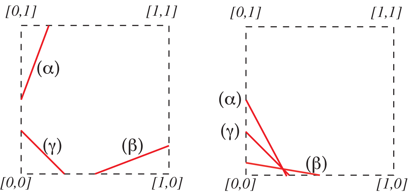
Let KαK_{\alpha}, KβK_{\beta} and KγK_{\gamma} be the components of the 33 chain link 𝒞3\mathcal{C}_{3}. The orientation of each component of 𝒞3\mathcal{C}_{3} is given in Figure 2(right). They bound the oriented disks FαF_{\alpha}, FβF_{\beta} and FγF_{\gamma} with 22 holes. Let us set α=[Fα]\alpha=[F_{\alpha}], β=[Fβ]\beta=[F_{\beta}], γ=[Fγ]∈H2​(N,∂N,ℤ)\gamma=[F_{\gamma}]\in H_{2}(N,\partial N;{\mathbb{Z}}). In [31], Thurston computed the unit ball UNU_{N} which is the the parallelepiped with vertices ±α\pm\alpha, ±β\pm\beta, ±γ\pm\gamma, ±(α+β+γ)\pm(\alpha+\beta+\gamma), see Figure 2(left). The set {α,β,γ}\{\alpha,\beta,\gamma\} is a basis of H2​(N,∂N,ℤ)H_{2}(N,\partial N;{\mathbb{Z}}), and the class x​α+y​β+z​γ∈H2​(N,∂N)x\alpha+y\beta+z\gamma\in H_{2}(N,\partial N) is denoted by (x,y,z)(x,y,z). Every top dimensional face on ∂UN\partial U_{N} is a fibered face because of the symmetries of H2​(N,∂N)H_{2}(N,\partial N), see Section 2.1. McMullen developed a general theory of the Teichmüller polynomial PΩP_{\Omega} for a fibered face Ω\Omega of fibered hyperbolic 3-manifolds, from which one can compute the dilatation λ⁡(a)\lambda(a) of each a∈i​n​t​(CΩ)a\in int(C_{\Omega}), see [29]. Let us pick the fibered face Δ\Delta on ∂UN\partial U_{N} as in Figure 2(left) with vertices (1,0,0)(1,0,0), (1,1,1)(1,1,1), (0,1,0)(0,1,0) and (0,0,−1)(0,0,-1). The Teichmüller polynomial PΔP_{\Delta} tells us that the dilatation λ⁡(a)=λ(x,y,z)\lambda(a)=\lambda_{(x,y,z)} of a primitive fibered class a=(x,y,z)∈i​n​t​(CΔ)a=(x,y,z)\in int(C_{\Delta}) is the largest real root of

(1.2) f(x,y,z)​(t)=tx+y−z−tx−ty−tx−z−ty−z+1,f_{(x,y,z)}(t)=t^{x+y-z}-t^{x}-t^{y}-t^{x-z}-t^{y-z}+1,

see [19, Theorem 3.1]. Thus, we have a reasonable source to compute dilatations systematically.

Refer to caption
Figure 2. (left) Thurston norm ball for N. (right) FαF_{\alpha}, FβF_{\beta}, FγF_{\gamma}. [arrows indicate the normal direction of oriented surfaces.]

To relate these data to ones on closed manifolds obtained from NN by Dehn filling, we prepare a few homological properties of NN. Denote by TαT_{\alpha} the torus which is the boundary of a regular neighborhood of KαK_{\alpha}. We define the tori TβT_{\beta} and TγT_{\gamma} in the same manner. For a primitive integral class a=(x,y,z)∈H2​(N,∂N)a=(x,y,z)\in H_{2}(N,\partial N), let us set ∂αFa=∂Fa∩Tα\partial_{\alpha}F_{a}=\partial F_{a}\cap T_{\alpha} which consists of the parallel simple closed curves on TαT_{\alpha}. We define ∂βFa\partial_{\beta}F_{a} and ∂γFa\partial_{\gamma}F_{a} in the same manner. We see that the slope of ∂αFa\partial_{\alpha}F_{a} (resp. ∂βFa\partial_{\beta}F_{a}, ∂γFa\partial_{\gamma}F_{a}) is given by bα​(a)=y+z−xb_{\alpha}(a)=\tfrac{y+z}{-x} (resp. bβ​(a)=z+x−yb_{\beta}(a)=\tfrac{z+x}{-y}, bγ​(a)=x+y−zb_{\gamma}(a)=\tfrac{x+y}{-z}). We call each of bα​(a)b_{\alpha}(a), bβ​(a)b_{\beta}(a), bγ​(a)b_{\gamma}(a) the boundary slope of aa.

For more detailed computation, we specify the cusp to be Dehn filled. Let N⁡(r)N(r) be the manifold obtained from NN by Dehn filling the cusp specified, say, by TβT_{\beta} along the slope r∈ℚr\in\mathbb{Q}. Then, there exists a natural injection ιβ:H2​(N⁡(r),∂N⁡(r))→H2​(N,∂N)\iota_{\beta}:H_{2}(N(r),\partial N(r))\rightarrow H_{2}(N,\partial N) whose image equals Sβ​(r)S_{\beta}(r), where

Sβ​(r)={(x,y,z)∈H2​(N,∂N)|−r​y=z+x},S_{\beta}(r)=\{(x,y,z)\in H_{2}(N,\partial N)\ |\ -ry=z+x\},

see Proposition 2.11. This implies that every slope r∈ℚr\in{\mathbb{Q}} can be realized by a boundary slope of some a∈H2​(N,∂N)a\in H_{2}(N,\partial N). It is known by [25] that N⁡(r)N(r) is hyperbolic if and only if r∈ℋ​y​p=ℚ∖{−3,−2,−1,0}r\in{\mathcal{H}yp}={\mathbb{Q}}\setminus\{-3,-2,-1,0\}. Choose such r∈ℋ​y​pr\in{\mathcal{H}yp}, and assume that a∈Sβ​(r)=Im​ιβa\in S_{\beta}(r)=\mathrm{Im}\,\iota_{\beta} is a fibered class in H2​(N,∂N)H_{2}(N,\partial N). Then, a¯=ιβ−1​(a)∈H2​(N⁡(r),∂N⁡(r))\overline{a}=\iota_{\beta}^{-1}(a)\in H_{2}(N(r),\partial N(r)) is also a fibered class of N⁡(r)N(r). This description enables us to compute the Thurston norm of N⁡(r)N(r), especially the unit ball and fibered faces, and hence to handle closed surface bundles obtained from NN by Dehn filling all cusps systematically.

What we further need for our purpose is to know a systematic method to compute entropies of monodromies on such bundles.

1.5. Main results

This paper concerns the small dilatation pseudo-Anosovs generated by the magic manifold NN with a very mild restriction which we describe below. Let Φ:F→F\Phi:F\rightarrow F be the monodromy of a fibration on NN, and let ϕ\phi be the mapping class of Φ\Phi. Then the fibration extends naturally to a fibration on the closed manifold obtained from NN by Dehn filling three cusps along boundary slopes of FF. Also, Φ\Phi extends to the monodromy Φ^:F^→F^\widehat{\Phi}:\widehat{F}\rightarrow\widehat{F} of the extended fibration, where the extended fiber F^\widehat{F} is obtained from FF by filing holes. Suppose that the stable foliation ℱ\mathcal{F} of Φ\Phi has the property such that each boundary component of FF has no 11 prong. Then ℱ\mathcal{F} extends canonically to the stable foliation ℱ^\widehat{\mathcal{F}} of Φ^\widehat{\Phi}, and ϕ^=[Φ^]\widehat{\phi}=[\widehat{\Phi}] becomes pseudo-Anosov (including Anosov) with the same dilatation as that of ϕ\phi. We consider the set ℳ\mathcal{M} of (pseudo-Anosov) mapping classes coming from fibrations of NN with this condition, i.e, if we let ℱ\mathcal{F} be the stable foliation associated to the fibration on NN, then ℱ\mathcal{F} has the property such that

(1.3) any boundary component of ​F​has no ​1​prong.\text{any boundary component of\ }F\ \text{has no\ }1\ \text{prong}.

We will see that this restriction is fairly mild (Lemmas 2.23 and 5.1). Let ℳ^\widehat{\mathcal{M}} be the set of extensions ϕ^\widehat{\phi} of ϕ∈ℳ\phi\in\mathcal{M} defined on the closed surfaces. For example, the pseudo-Anosov Φg​(r):Σg→Σg\Phi_{g}(r):\varSigma_{g}\rightarrow\varSigma_{g} in Theorem 1.3 enjoys [Φg​(r)]∈ℳ^[\Phi_{g}(r)]\in\widehat{\mathcal{M}} for large gg, see [20, Lemma 4.8].

Let δ^g\widehat{\delta}_{g} be the minimum among dilatations of elements in ℳ^∩Mod⁡(Σg)\widehat{\mathcal{M}}\,\cap\,\mathrm{Mod}(\varSigma_{g}). Clearly δg≤δ^g\delta_{g}\leq\widehat{\delta}_{g}. The equality is achieved when g=2g=2 [15]. We prove that the limit of g​log⁡δ^gg\log\widehat{\delta}_{g} exists and it equals the number which we encountered in Theorem 1.3.

Theorem 1.4.
  1. (1)

    We have limg→∞g​log⁡δ^g=log⁡(3+52)\displaystyle\lim_{g\to\infty}g\log\widehat{\delta}_{g}=\log(\tfrac{3+\sqrt{5}}{2}).

  2. (2)

    For large gg, δ^g\widehat{\delta}_{g} is achieved by the monodromy of some Σg\varSigma_{g}-bundle over the circle obtained from either N⁡(3−2)N(\tfrac{3}{-2}) or N⁡(1−2)N(\tfrac{1}{-2}) by Dehn filling both cusps.

More precisely, the following holds. (See also Remark 3.18.) For large gg such that g≡0,1,5,6,7,9(mod10)g\equiv 0,1,5,6,7,9\pmod{10} (resp. large gg such that g≡3,8(mod10)g\equiv 3,8\pmod{10}), δ^g\widehat{\delta}_{g} is achieved by the monodromy of some Σg\varSigma_{g}-bundle over the circle obtained from N⁡(3−2)N(\tfrac{3}{-2}) (resp. N⁡(1−2)N(\tfrac{1}{-2})) by Dehn filling both cusps.

We know from [20, Proposition 4.37] that for g=8,13g=8,13, δ^g\widehat{\delta}_{g} cannot be achieved by the monodromy of any Σg\varSigma_{g}-bundle over the circle obtained from either N⁡(3−2)N(\tfrac{3}{-2}) or N⁡(1−2)N(\tfrac{1}{-2}) by Dehn filling. In fact, the manifold N⁡(4−3,25−17,−5)N(\tfrac{4}{-3},\tfrac{25}{-17},-5) (resp. N⁡(29−27,5−3,−6)N(\tfrac{29}{-27},\tfrac{5}{-3},-6)) is a Σ8\varSigma_{8}-bundle (resp. a Σ13\varSigma_{13}-bundle) over the circle, where N⁡(r1,r2,r3)N(r_{1},r_{2},r_{3}) is the closed manifold obtained from NN by Dehn filling all cusps along the slopes r1r_{1}, r2r_{2} and r3r_{3}. Its dilatation is smaller than that of any Σ8\varSigma_{8}-bundle (resp. Σ13\varSigma_{13}-bundle) over the circle obtained from either N⁡(3−2)N(\tfrac{3}{-2}) or N⁡(1−2)N(\tfrac{1}{-2}) by Dehn filling. Theorem 1.4 says that if gg is large, then among elements of ℳ^\widehat{\mathcal{M}}, the pseudo-Anosovs defined on Σg\varSigma_{g} with the smallest dilatation are the same examples identified by Hironaka [15], Aabor-Dunfield [1] and Kin-Takasawa [20].

However, we can find new examples in ℳ^\widehat{\mathcal{M}} defined on Σg\varSigma_{g} with orientable invariant foliations when g≡0(mod6)g\equiv 0\pmod{6}. Let ℳ^+\widehat{\mathcal{M}}^{+} be the set of pseudo-Anosov elements of ℳ^\widehat{\mathcal{M}} with orientable invariant foliations. Let δ^g+\widehat{\delta}_{g}^{+} be the minimum among dilatations of elements in ℳ^+∩Mod⁡(Σg)\widehat{\mathcal{M}}^{+}\,\cap\,\mathrm{Mod}(\varSigma_{g}). Since ℳ^+∩Mod⁡(Σg)≠∅\widehat{\mathcal{M}}^{+}\,\cap\,\mathrm{Mod}(\varSigma_{g})\neq\emptyset for g≥2g\geq 2 (Lemma 3.19), δ^g+\widehat{\delta}_{g}^{+} is well-defined. Clearly δg≤δg+≤δ^g+\delta_{g}\leq\delta_{g}^{+}\leq\widehat{\delta}_{g}^{+}.

The following describes the asymptotic behavior of δ^g+\widehat{\delta}_{g}^{+}’s in the case g≢0(mod6)g\not\equiv 0\pmod{6}.

Theorem 1.5.
  1. (1)

    We have limg≢0(mod6)g→∞g​log⁡δ^g+=log⁡(3+52)\displaystyle\lim_{\begin{subarray}{c}g\not\equiv 0\pmod{6}\\ g\to\infty\end{subarray}}g\log\widehat{\delta}^{+}_{g}=\log(\tfrac{3+\sqrt{5}}{2}).

  2. (2)

    For large gg such that g≡2,4(mod6)g\equiv 2,4\pmod{6} or g≡3(mod10)g\equiv 3\pmod{10}, δ^g+\widehat{\delta}^{+}_{g} is achieved by the monodromy of some Σg\varSigma_{g}-bundle over the circle obtained from N⁡(1−2)N(\tfrac{1}{-2}) by Dehn filling both cusps.

  3. (3)

    For large gg such that g≡1,5,7,9(mod10)g\equiv 1,5,7,9\pmod{10}, δ^g+\widehat{\delta}^{+}_{g} is achieved by the monodromy of some Σg\varSigma_{g}-bundle over the circle obtained from N⁡(3−2)N(\tfrac{3}{-2}) by Dehn filling both cusps.

Theorem 1.5(1) leads to the following estimate, which was proved by Hironaka first [15].

lim supg≢0(mod6)g→∞g​log⁡δg+≤log⁡(3+52).\limsup_{\begin{subarray}{c}g\not\equiv 0\pmod{6}\\ g\to\infty\end{subarray}}g\log\delta_{g}^{+}\leq\log(\tfrac{3+\sqrt{5}}{2}).

If g≢0(mod6)g\not\equiv 0\pmod{6} is large, then elements of ℳ^+\widehat{\mathcal{M}}^{+} defined on Σg\varSigma_{g} with the smallest dilatation are the same examples discovered in [15, 1, 20].

In the case g≡0(mod6)g\equiv 0\pmod{6}, there exist no examples of elements in ℳ^+\widehat{\mathcal{M}}^{+} defined on Σg\varSigma_{g} which occur as monodromies of fibrations on manifolds obtained from N⁡(1−2)N(\tfrac{1}{-2}) or N⁡(3−2)N(\tfrac{3}{-2}) by Dehn filling both cusps [15, 1, 20]. To the best of our knowledge, the smallest known upper bound on δg+\delta_{g}^{+} for g≡0(mod6)g\equiv 0\pmod{6} is

(1.4) δg+≤λ(g,g,−1),\delta_{g}^{+}\leq\lambda_{(g,g,-1)},

where λ(g,g,−1)\lambda_{(g,g,-1)} is the largest root of f(g,g,−1)​(t)=t2​g+1−2​tg+1−2​tg+1f_{(g,g,-1)}(t)=t^{2g+1}-2t^{g+1}-2t^{g}+1, see [28, 16]. By using the bound (1.4), Minakawa and independently Hironaka-Kin proved that

(1.5) g​log⁡δg+≤log⁡(2+3)≈1.3169.g\log\delta_{g}^{+}\leq\log(2+\sqrt{3})\approx 1.3169.

We would like to point out that the set ℳ^+\widehat{\mathcal{M}}^{+} could be a source to provide a sharper upper bound on δg+\delta_{g}^{+} than the bound (1.4) in the case g≡0(mod6)g\equiv 0\pmod{6}. In fact, we will find elements of ℳ^+\widehat{\mathcal{M}}^{+} defined on Σg\varSigma_{g} for g≡6(mod12)g\equiv 6\pmod{12} whose normalized entropies go to 4​log⁡δ​(D5)4\log\delta(D_{5}) as gg goes to ∞\infty, see Lemmas 3.22 and 3.23. These examples occur as monodromies of fibrations on manifolds obtained from N⁡(4)N(4) or N⁡(−6)N(-6) by Dehn filling both cusps. As a corollary, we have

Theorem 1.6.

lim supg≡6(mod12)g→∞g​log⁡δg+≤2​log⁡δ⁡(D5)≈1.0870\displaystyle\limsup_{\begin{subarray}{c}g\equiv 6\pmod{12}\\ g\to\infty\end{subarray}}g\log\delta^{+}_{g}\leq 2\log\delta(D_{5})\approx 1.0870.

By using our examples, we give the following upper bound on δg+\delta_{g}^{+} for g≡6(mod12)g\equiv 6\pmod{12} which is sharper than the previous one (1.4). (See also Table 1.)

Theorem 1.7 (Upper bound on δg+\delta_{g}^{+} for g≡6(mod12)g\equiv 6\pmod{12}).
  1. (1)

    δg+≤λ(3​g2+1,3​g2−1,g2)\delta_{g}^{+}\leq\lambda_{(\tfrac{3g}{2}+1,\tfrac{3g}{2}-1,\tfrac{g}{2})} if g≡6,30,42,54,78(mod84)g\equiv 6,30,42,54,78\pmod{84}.

  2. (2)

    δg+≤λ(g+2,g−2,−g2)\delta_{g}^{+}\leq\lambda_{(g+2,g-2,-\tfrac{g}{2})} if g≡18,66(mod84)g\equiv 18,66\pmod{84}.

In the case g≡0(mod12)g\equiv 0\pmod{12}, we improve the bound (1.4) for many gg, see Table 1.

Table 1. upper bound on δg+\delta_{g}^{+} for 6≤g≤2166\leq g\leq 216 such that g≡0(mod6)g\equiv 0\pmod{6}. [the bounds on δg+\delta_{g}^{+} on the left in the case g≡6(mod12)g\equiv 6\pmod{12} come from Theorem 1.7. in the case g≡0(mod12)g\equiv 0\pmod{12} and g>12g>12, the bounds on δg+\delta_{g}^{+} on the left are given by elements of ℳ^+\widehat{\mathcal{M}}^{+} which occur as monodromies of fibrations on manifolds obtained from N⁡(5−4)N(\tfrac{5}{-4}) by Dehn filling both cusps.]

|gupper bound on ​δg+upper bound on ​δg+​in [28, 16]6λ(10,8,3)≈1.20189λ(6,6,−1)≈1.2257112λ(12,20,3)≈1.10240λ(12,12,−1)≈1.1112418λ(20,16,−9)≈1.06276λ(18,18,−1)≈1.0738224λ(32,28,3)≈1.04757λ(24,24,−1)≈1.0552430λ(46,44,15)≈1.03692λ(30,30,−1)≈1.0441336λ(50,52,15)≈1.03148λ(36,36,−1)≈1.0367442λ(64,62,21)≈1.02622λ(42,42,−1)≈1.0314748λ(66,68,19)≈1.02367λ(48,48,−1)≈1.0275254λ(82,80,27)≈1.02033λ(54,54,−1)≈1.0244660λ(80,76,15)≈1.01903λ(60,60,−1)≈1.0220066λ(68,64,−33)≈1.01661λ(66,66,−1)≈1.0200072λ(96,92,19)≈1.01586λ(72,72,−1)≈1.0183378λ(118,116,39)≈1.01403λ(78,78,−1)≈1.0169184λ(114,116,31)≈1.01357λ(84,84,−1)≈1.0157090λ(136,134,45)≈1.01215λ(90,90,−1)≈1.0146596λ(132,140,43)≈1.01190λ(96,96,−1)≈1.01374102λ(104,100,−51)≈1.01071λ(102,102,−1)≈1.01293108λ(146,148,39)≈1.01057λ(108,108,−1)≈1.01221114λ(172,170,57)≈1.00958λ(114,114,−1)≈1.01156120λ(164,172,51)≈1.00952λ(120,120,−1)≈1.01098126λ(190,188,63)≈1.00841λ(126,126,−1)≈1.01046132λ(174,164,31)≈1.00869λ(132,132,−1)≈1.00998138λ(208,206,69)≈1.00790λ(138,138,−1)≈1.00955144λ(194,196,51)≈1.00793λ(144,144,−1)≈1.00915150λ(152,148,−75)≈1.00727λ(150,150,−1)≈1.00878156λ(210,212,55)≈1.00732λ(156,1566,−1)≈1.00845162λ(244,,242,81)≈1.00673λ(162,162,−1)≈1.00813168λ(228,236,67)≈1.00680λ(168,168,−1)≈1.00784174λ(262,260,87)≈1.00626λ(174,174,−1)≈1.00757180λ(240,236,55)≈1.00635λ(180,180,−1)≈1.00732186λ(188,184,−93)≈1.00586λ(186,186,−1)≈1.00708192λ(258,260,67)≈1.00595λ(192,192,−1)≈1.00686198λ(298,296,99)≈1.00550λ(198,198,−1)≈1.00665204λ(276,284,79)≈1.00560λ(204,204,−1)≈1.00646210λ(316,314,105)≈1.00519λ(210,210,−1)≈1.00627216λ(290,292,75)≈1.00529λ(216,216,−1)≈1.00610|\left|\begin{array}[]{c|c|c}\hline\cr g&\mbox{upper bound on\ }\delta_{g}^{+}&\mbox{upper bound on\ }\delta_{g}^{+}\ \mbox{in \cite[cite]{[\@@bibref{}{Minakawa,HK}{}{}]}}\\ \hline\cr\hline\cr 6&\lambda_{(10,8,3)}\approx 1.20189&\lambda_{(6,6,-1)}\approx 1.22571\\ \hline\cr 12&\lambda_{(12,20,3)}\approx 1.10240&\lambda_{(12,12,-1)}\approx 1.11124\\ \hline\cr 18&\lambda_{(20,16,-9)}\approx 1.06276&\lambda_{(18,18,-1)}\approx 1.07382\\ \hline\cr 24&\lambda_{(32,28,3)}\approx 1.04757&\lambda_{(24,24,-1)}\approx 1.05524\\ \hline\cr 30&\lambda_{(46,44,15)}\approx 1.03692&\lambda_{(30,30,-1)}\approx 1.04413\\ \hline\cr 36&\lambda_{(50,52,15)}\approx 1.03148&\lambda_{(36,36,-1)}\approx 1.03674\\ \hline\cr 42&\lambda_{(64,62,21)}\approx 1.02622&\lambda_{(42,42,-1)}\approx 1.03147\\ \hline\cr 48&\lambda_{(66,68,19)}\approx 1.02367&\lambda_{(48,48,-1)}\approx 1.02752\\ \hline\cr 54&\lambda_{(82,80,27)}\approx 1.02033&\lambda_{(54,54,-1)}\approx 1.02446\\ \hline\cr 60&\lambda_{(80,76,15)}\approx 1.01903&\lambda_{(60,60,-1)}\approx 1.02200\\ \hline\cr 66&\lambda_{(68,64,-33)}\approx 1.01661&\lambda_{(66,66,-1)}\approx 1.02000\\ \hline\cr 72&\lambda_{(96,92,19)}\approx 1.01586&\lambda_{(72,72,-1)}\approx 1.01833\\ \hline\cr 78&\lambda_{(118,116,39)}\approx 1.01403&\lambda_{(78,78,-1)}\approx 1.01691\\ \hline\cr 84&\lambda_{(114,116,31)}\approx 1.01357&\lambda_{(84,84,-1)}\approx 1.01570\\ \hline\cr 90&\lambda_{(136,134,45)}\approx 1.01215&\lambda_{(90,90,-1)}\approx 1.01465\\ \hline\cr 96&\lambda_{(132,140,43)}\approx 1.01190&\lambda_{(96,96,-1)}\approx 1.01374\\ \hline\cr 102&\lambda_{(104,100,-51)}\approx 1.01071&\lambda_{(102,102,-1)}\approx 1.01293\\ \hline\cr 108&\lambda_{(146,148,39)}\approx 1.01057&\lambda_{(108,108,-1)}\approx 1.01221\\ \hline\cr 114&\lambda_{(172,170,57)}\approx 1.00958&\lambda_{(114,114,-1)}\approx 1.01156\\ \hline\cr 120&\lambda_{(164,172,51)}\approx 1.00952&\lambda_{(120,120,-1)}\approx 1.01098\\ \hline\cr 126&\lambda_{(190,188,63)}\approx 1.00841&\lambda_{(126,126,-1)}\approx 1.01046\\ \hline\cr 132&\lambda_{(174,164,31)}\approx 1.00869&\lambda_{(132,132,-1)}\approx 1.00998\\ \hline\cr 138&\lambda_{(208,206,69)}\approx 1.00790&\lambda_{(138,138,-1)}\approx 1.00955\\ \hline\cr 144&\lambda_{(194,196,51)}\approx 1.00793&\lambda_{(144,144,-1)}\approx 1.00915\\ \hline\cr 150&\lambda_{(152,148,-75)}\approx 1.00727&\lambda_{(150,150,-1)}\approx 1.00878\\ \hline\cr 156&\lambda_{(210,212,55)}\approx 1.00732&\lambda_{(156,1566,-1)}\approx 1.00845\\ \hline\cr 162&\lambda_{(244,,242,81)}\approx 1.00673&\lambda_{(162,162,-1)}\approx 1.00813\\ \hline\cr 168&\lambda_{(228,236,67)}\approx 1.00680&\lambda_{(168,168,-1)}\approx 1.00784\\ \hline\cr 174&\lambda_{(262,260,87)}\approx 1.00626&\lambda_{(174,174,-1)}\approx 1.00757\\ \hline\cr 180&\lambda_{(240,236,55)}\approx 1.00635&\lambda_{(180,180,-1)}\approx 1.00732\\ \hline\cr 186&\lambda_{(188,184,-93)}\approx 1.00586&\lambda_{(186,186,-1)}\approx 1.00708\\ \hline\cr 192&\lambda_{(258,260,67)}\approx 1.00595&\lambda_{(192,192,-1)}\approx 1.00686\\ \hline\cr 198&\lambda_{(298,296,99)}\approx 1.00550&\lambda_{(198,198,-1)}\approx 1.00665\\ \hline\cr 204&\lambda_{(276,284,79)}\approx 1.00560&\lambda_{(204,204,-1)}\approx 1.00646\\ \hline\cr 210&\lambda_{(316,314,105)}\approx 1.00519&\lambda_{(210,210,-1)}\approx 1.00627\\ \hline\cr 216&\lambda_{(290,292,75)}\approx 1.00529&\lambda_{(216,216,-1)}\approx 1.00610\\ \hline\cr\end{array}\right|

Section 3.5 concerns the monodromies of fibrations on the Whitehead link exterior N⁡(1)N(1). The manifold N⁡(1)N(1) is very special among other N⁡(r)N(r)’s. It is the only manifold among the N⁡(r)N(r)’s which admits fibers with arbitrarily many boundary components (Lemma 5.2). Moreover the invariant foliation of the monodromy of each fibration on N⁡(1)N(1) has the property such that each boundary component of the fiber has a 11 prong. (Remark 3.29). We shall show in Section 3.5 that there exists the monodromy Φn:Σ1,n→Σ1,n\Phi_{n}:\varSigma_{1,n}\rightarrow\varSigma_{1,n} of a particular fibration on N⁡(1)N(1) whose normalized entropy tends to 2​log⁡δ​(D4)2\log\delta(D_{4}) as nn tends to ∞\infty (Proposition 3.30 and Lemma 3.31). Thus we have

Theorem 1.8.

lim supn→∞n​log⁡δ1,n≤2​log⁡δ⁡(D4)\displaystyle\limsup_{n\to\infty}\,n\log\delta_{1,n}\leq 2\log\delta(D_{4}).

This implies the upper bound lim supn→∞n​log⁡δ1,n≤2​log⁡9\displaystyle\limsup_{n\to\infty}\,n\log\delta_{1,n}\leq 2\log 9 by Tsai, see [34, Section 3.2.1 and Theorem 3.2.2].

1.6. Thurston norm equivalence, entropy equivalence on manifolds N⁡(r)N(r)

In the course of analyzing the magic manifold, we discovered many “twins” among the N⁡(r)N(r)’s. The particular ones are N⁡(3−2)N(\tfrac{3}{-2}) and N⁡(1−2)N(\tfrac{1}{-2}) which will be critical in the proof of Theorem 1.4. They are different manifolds but have common properties from entropy computational viewpoints. To formulate ideas, we say that 33-manifolds MM and M′M^{\prime} are Thurston norm equivalent, denoted by

M​∼T​M′,M\underset{\mathrm{T}}{\sim}M^{\prime},

if there exists an isomorphism f:H2​(M,∂M,ℤ)→H2​(M′,∂M′,ℤ)f:H_{2}(M,\partial M;{\mathbb{Z}})\rightarrow H_{2}(M^{\prime},\partial M^{\prime};{\mathbb{Z}}) which preserves the Thurston norm, i.e, ‖a‖=‖f⁡(a)‖\|a\|=\|f(a)\| for any a∈H2​(M,∂M,ℤ)a\in H_{2}(M,\partial M;{\mathbb{Z}}). We call such ff the Thurston norm preserving isomorphism. For example N⁡(r)​∼T​N​(−2−r)N(r)\underset{\mathrm{T}}{\sim}N(-2-r) when r,−2−r∈ℋ​y​pr,-2-r\in{\mathcal{H}yp} (Proposition 2.20). We introduce two more equivalence relations, both called the entropy equivalence, of which the precise definitions are given in Section 2.5.1. The first one is defined on the pairs (M,Ω)(M,\Omega), where MM is a fibered 33-manifold and Ω\Omega is its fibered face. Namely, (M,Ω)(M,\Omega) and (M′,Ω′)(M^{\prime},\Omega^{\prime}) are entropy equivalent, denoted by

(M,Ω)​∼ent​(M′,Ω′),(M,\Omega)\underset{\mathrm{ent}}{\sim}(M^{\prime},\Omega^{\prime}),

if there exists a Thurston norm preserving isomorphism f:H2​(M,∂M,ℤ)→H2​(M′,∂M′,ℤ)f:H_{2}(M,\partial M;{\mathbb{Z}})\rightarrow H_{2}(M^{\prime},\partial M^{\prime};{\mathbb{Z}}) such that ff maps i​n​t​(CΩ​(ℤ))int(C_{\Omega}(\mathbb{Z})) to i​n​t​(CΩ′​(ℤ))int(C_{\Omega^{\prime}}(\mathbb{Z})) preserving the entropy function. In particular (M,Ω)​∼ent​(M′,Ω′)(M,\Omega)\underset{\mathrm{ent}}{\sim}(M^{\prime},\Omega^{\prime}) implies that min⁡Ent⁡(M,Ω)=min⁡Ent⁡(M′,Ω′)\min\mathrm{Ent}(M,\Omega)=\min\mathrm{Ent}(M^{\prime},\Omega^{\prime}). The second equivalence relation is defined on the fibered 33-manifolds. Fibered 33-manifolds MM and M′M^{\prime} are entropy equivalent, denoted by

M​∼ent​M′,M\underset{\mathrm{ent}}{\sim}M^{\prime},

if there exists a Thurston norm preserving isomorphism f:H2​(M,∂M,ℤ)→H2​(M′,∂M′,ℤ)f:H_{2}(M,\partial M;{\mathbb{Z}})\rightarrow H_{2}(M^{\prime},\partial M^{\prime};{\mathbb{Z}}) such that ff preserves both fibered classes and the entropy functions. If M​∼ent​M′M\underset{\mathrm{ent}}{\sim}M^{\prime}, then min⁡Ent⁡(M)=min⁡Ent⁡(M′)\min\mathrm{Ent}(M)=\min\mathrm{Ent}(M^{\prime}). We shall prove in Theorem 2.26 that

(N⁡(2),ΩS)​∼ent​(N⁡(3−2),ΩA)​∼ent​(N⁡(1−2),ΩA).(N(2),\Omega_{S})\underset{\mathrm{ent}}{\sim}(N(\tfrac{3}{-2}),\Omega_{A})\underset{\mathrm{ent}}{\sim}(N(\tfrac{1}{-2}),\Omega_{A}).

For the definition of fibered faces ΩS\Omega_{S} and ΩA\Omega_{A}, see Section 2.5.2. We also prove that N⁡(r)​∼ent​N​(−2−r)N(r)\underset{\mathrm{ent}}{\sim}N(-2-r) for ‘almost all’ r∈ℋ​y​pr\in{\mathcal{H}yp}, see Theorem 2.26. This is derived from the symmetry of the Thurston norm ball and the symmetry of the entropy function of NN. In particular

N⁡(3−2)​∼ent​N​(1−2).N(\tfrac{3}{-2})\underset{\mathrm{ent}}{\sim}N(\tfrac{1}{-2}).

Recall that the quantity min⁡Ent\min\mathrm{Ent} is defined to be the minimum of the normalized entropies of the classes in ⋃Ωi​n​t​(CΩ)\displaystyle\bigcup_{\Omega}int(C_{\Omega}), where Ω\Omega is taken over all fibered faces of MM. The number log⁡(3+52)\log(\tfrac{3+\sqrt{5}}{2}) in Theorem 1.3 appears in the equalities

min⁡Ent⁡(N⁡(3−2))=min⁡Ent⁡(N⁡(1−2))=min⁡Ent⁡(N⁡(2),ΩS)=2​log⁡(3+52).\min\mathrm{Ent}(N(\tfrac{3}{-2}))=\min\mathrm{Ent}(N(\tfrac{1}{-2}))=\min\mathrm{Ent}(N(2),\Omega_{S})=2\log(\tfrac{3+\sqrt{5}}{2}).

1.7. Question by Lanneau-Thiffeault

Let kk and ℓ\ell be integers such that 0<ℓ<k0<\ell<k. We consider following fibered classes in i​n​t​(CΔ)int(C_{\Delta}):

(2​k±ℓ,2​k±2​ℓ,k±2​ℓ)∈Sβ​(3−2),(k,2​k±2​ℓ,±ℓ)∈Sβ​(1−2),(k±ℓ,k∓ℓ,−k)∈Sγ​(2).(2k\pm\ell,2k\pm 2\ell,k\pm 2\ell)\in S_{\beta}(\tfrac{3}{-2}),\ (k,2k\pm 2\ell,\pm\ell)\in S_{\beta}(\tfrac{1}{-2}),\ (k\pm\ell,k\mp\ell,-k)\in S_{\gamma}(2).

By using the Teichmüller polynomial (1.2), we see that the dilatation of each fibered class above is equal to the largest real root λ(k,ℓ)\lambda_{(k,\ell)} of the following Lanneau-Thiffeault polynomial

f(k,ℓ)​(t)=t2​k−tk+ℓ−tk−tk−ℓ+1.f_{(k,\ell)}(t)=t^{2k}-t^{k+\ell}-t^{k}-t^{k-\ell}+1.

(In fact, f(k,ℓ)​(t)f_{(k,\ell)}(t) is a common factor of f(2​k±ℓ,2​k±2​ℓ,k±2​ℓ)​(t)f_{(2k\pm\ell,2k\pm 2\ell,k\pm 2\ell)}(t), f(k,2​k±2​ℓ,±ℓ)​(t)f_{(k,2k\pm 2\ell,\pm\ell)}(t) and f(k±ℓ,k∓ℓ,−k)​(t)f_{(k\pm\ell,k\mp\ell,-k)}(t).)

It is known that δ2+=λ(2,1)\delta_{2}^{+}=\lambda_{(2,1)}, δ4+=λ(4,1)\delta_{4}^{+}=\lambda_{(4,1)}, δ6+≥λ(6,1)\delta_{6}^{+}\geq\lambda_{(6,1)}, δ8+=λ(8,1)\delta_{8}^{+}=\lambda_{(8,1)}, see [36, 22, 15]. Motivated by these results, Lanneau and Thiffeault asked the following.

Question 1.9 ([22]).

For gg even, is δg+\delta_{g}^{+} equal to λ(g,1)\lambda_{(g,1)}?

We consider Question 1.9 in the set ℳ^+\widehat{\mathcal{M}}^{+}. The results in this paper imply that there exists a gap between δ^g+\widehat{\delta}^{+}_{g} and λ(g,1)\lambda_{(g,1)} for large gg such that g≡0(mod6)g\equiv 0\pmod{6}.

Theorem 1.10.
  1. (1)

    We fix any ϵ>0\epsilon>0 so that 1.97475−ϵ>2​log⁡(3+52)1.97475-\epsilon>2\log(\tfrac{3+\sqrt{5}}{2}). For large gg such that g≡0(mod6)g\equiv 0\pmod{6}, we have δ^g+>λ(g,1)\widehat{\delta}^{+}_{g}>\lambda_{(g,1)} and

    |χ⁡(Σg)|​log⁡δ^g+>1.97475−ϵ>2​log⁡(3+52).|\chi(\varSigma_{g})|\log\widehat{\delta}^{+}_{g}>1.97475-\epsilon>2\log(\tfrac{3+\sqrt{5}}{2}).
  2. (2)

    δ^g+=λ(g,1)\widehat{\delta}^{+}_{g}=\lambda_{(g,1)} for large gg such that g≡2,4(mod6)g\equiv 2,4\pmod{6}.

1.8. Idea of proofs and conjectures

This subsection describes the outline of the proof of Theorem 1.4. (The proof of Theorem 1.5 is similar.) First, let us recall the approach to (1.1) by Hironaka [15], Aaber-Dunfield [1] and Kin-Takasawa [20]. Take a particular single 22-cusped hyperbolic fibered 33-manifold MM (which is either N⁡(1−2),N⁡(3−2)N(\tfrac{1}{-2}),N(\tfrac{3}{-2}) or N⁡(2)N(2).) Compute the Teichmüller polynomial PΩP_{\Omega} and min⁡Ent⁡(M,Ω)\min\mathrm{Ent}(M,\Omega) (=2​log⁡(3+52)=2\log(\tfrac{3+\sqrt{5}}{2}) in this case) for a fibered face Ω\Omega of MM. Then determine the topological type of each fiber FF such that [F]∈i​n​t​(CΩ)[F]\in int(C_{\Omega}). We can find a fiber FgF_{g} of genus gg for large gg which enjoys the following. The ray of [Fg][F_{g}] goes to the ray whose normalized entropy Ent\mathrm{Ent} achieves min⁡Ent⁡(M,Ω)\min\mathrm{Ent}(M,\Omega) as gg goes to ∞\infty. (Then Ent⁡([Fg])\mathrm{Ent}([F_{g}]) goes to min⁡Ent⁡(M,Ω)\min\mathrm{Ent}(M,\Omega) as gg goes to ∞\infty.) Moreover, the number of boundary components of FgF_{g} is bounded by some constant. Finally check that the stable foliation for the monodromy of the fibration associated to [Fg][F_{g}] satisfies that each boundary component of FgF_{g} has no 11 prong. Then we obtain the equality in Theorem 1.3 which implies (1.1).

Compared to the above approach, a difficulty for the proof of Theorem 1.4 is that for each r∈ℋ​y​p∖{1}r\in{\mathcal{H}yp}\setminus\{1\}, the manifold N⁡(r)N(r) has a fiber of arbitrarily large genus. Because of this, it is not clear which manifold N⁡(r)N(r) we should look in. Thus it is not a straightforward task to identify a primitive fibered class ag∈H2​(N,∂N)a_{g}\in H_{2}(N,\partial N) such that ϕag∈ℳ\phi_{a_{g}}\in\mathcal{M} and δ^g\widehat{\delta}_{g} is achieved by ϕ^ag∈ℳ^∩Mod⁡(Σg)\widehat{\phi}_{a_{g}}\in\widehat{\mathcal{M}}\cap\mathrm{Mod}(\varSigma_{g}). Also it is not obvious at all that one of the boundary slopes of aga_{g} becomes a constant for large gg. (As we will see, one of the boundary slopes of aga_{g} must be in {−4,3−2,1−2,2}\{-4,\frac{3}{-2},\frac{1}{-2},2\} for large gg.) The key observation to prove Theorem 1.4 is

Theorem 1.11.

For r∈ℋ​y​pr\in{\mathcal{H}yp}, let Ω\Omega be any fibered face of N⁡(r)N(r) which enjoys the following.

(∗)(*) Let a∈Sβ​(r)a\in S_{\beta}(r) be a primitive fibered class of NN such that a¯∈i​n​t​(CΩ)\overline{a}\in int(C_{\Omega}). Let Φa:Fa→Fa\Phi_{a}:F_{a}\rightarrow F_{a} be the monodromy of the fibration associated to aa. Then the stable foliation ℱa\mathcal{F}_{a} of Φa\Phi_{a} has the property such that any boundary component of FaF_{a} lying on TβT_{\beta} has no 11 prong.

Then

  1. (1)

    min⁡Ent⁡(N⁡(1),Ω)=2​log⁡δ⁡(D4)≈1.6628\min\mathrm{Ent}(N(1),\Omega)=2\log\delta(D_{4})\approx 1.6628,

  2. (2)

    if r=−4,3−2,1−2,2r=-4,\tfrac{3}{-2},\tfrac{1}{-2},2, then min⁡Ent⁡(N⁡(r),Ω)=2​log⁡δ⁡(D3)=2​log⁡(3+52)≈1.9248\min\mathrm{Ent}(N(r),\Omega)=2\log\delta(D_{3})=2\log(\tfrac{3+\sqrt{5}}{2})\approx 1.9248, and

  3. (3)

    if r≠−4,3−2,1−2,1,2r\neq-4,\tfrac{3}{-2},\tfrac{1}{-2},1,2, then min⁡Ent⁡(N⁡(r),Ω)>1.97475\min\mathrm{Ent}(N(r),\Omega)>1.97475.

We remark here that for any r∈ℋ​y​pr\in{\mathcal{H}yp}, there exists Ω\Omega having the condition (∗)(*) (Proposition 2.24). Thus, there are no slopes rr for which we cannot apply Theorem 1.11. Also, since the three claims in Theorem 1.11 cover all slopes r∈ℋ​y​pr\in{\mathcal{H}yp}, the conclusions we could draw from Theorem 1.11 are expected to be fairly sharp.

To see this, consider the set of pairs

𝒟={(N(r),Ω)|r∈ℋyp,Ωis a fibered face of N⁡(r) with (∗)}.\mathcal{D}=\{(N(r),\Omega)\,|\,r\in{\mathcal{H}yp},\,\Omega\;\;\text{is a fibered face of $N(r)$ with $(*)$}\}.

Theorem 1.11 shows for instance that there exist a minimum and a second minimum of

{min⁡Ent⁡(N⁡(r),Ω)|(N⁡(r),Ω)∈𝒟}\{\min\mathrm{Ent}(N(r),\Omega)\,|\,(N(r),\Omega)\in\mathcal{D}\}

and they are 2​log⁡δ​(D4)2\log\delta(D_{4}) and 2​log⁡δ​(D3)2\log\delta(D_{3}) respectively. The minimum is attained only by N⁡(1)N(1) and the second minimum is attained by N⁡(r)N(r) for r∈{−4,3−2,1−2,2}r\in\{-4,\frac{3}{-2},\frac{1}{-2},2\}. Furthermore, if r∉{−4,3−2,1−2,1,2}r\not\in\{-4,\frac{3}{-2},\frac{1}{-2},1,2\}, then Theorem 1.11(3) says that min⁡Ent⁡(N⁡(r),Ω)\min\mathrm{Ent}(N(r),\Omega) is greater than the second minimum with a uniform gap.

The condition (∗)(*) on one boundary component, TβT_{\beta}, of NN is a weaker version of the condition (1.3) on all three boundary components. If Ω\Omega enjoys (∗)(*), then the dilatation of a∈Sβ​(r)a\in S_{\beta}(r) for NN equals the dilatation of a¯\overline{a} for N⁡(r)N(r). Thus one can compute the dilatation of a¯\overline{a} by using the Teichmüller polynomial of NN. In Section 2.2, we shall see that the entropy function for NN has symmetries. This property together with the strict concavity of 1ent\tfrac{1}{\mathrm{ent}} works well in the proof of Theorem 1.11.

Outline of the proof of Theorem 1.4.

It is known that N⁡(−4)≃N⁡(3−2)N(-4)\simeq N(\tfrac{3}{-2}) and N⁡(1)≃N(1)\simeq the Whitehead link exterior, see [25]. Recall that aga_{g} is a primitive fibered class of H2​(N,∂N)H_{2}(N,\partial N) such that ϕag∈ℳ\phi_{a_{g}}\in\mathcal{M} and δ^g\widehat{\delta}_{g} is achieved by ϕ^ag∈ℳ^∩Mod⁡(Σg)\widehat{\phi}_{a_{g}}\in\widehat{\mathcal{M}}\cap\mathrm{Mod}(\varSigma_{g}). There exists such a fibered class aga_{g} for any g≥3g\geq 3. (In fact, the existence of the fiber of the fibration of genus gg for any g≥3g\geq 3 is guaranteed by Theorem 1.3. By [20, Lemma 4.7], one sees that the monodromy of this fibration is in the set ℳ\mathcal{M}.)

Since we know from the computation that N⁡(1)N(1) has no fiber of genus greater than 11, aga_{g} does not have a boundary slope 11 for g≥2g\geq 2. On the other hand, each of three manifolds N⁡(−4)≃N⁡(3−2)N(-4)\simeq N(\tfrac{3}{-2}), N⁡(1−2)N(\tfrac{1}{-2}) and N⁡(2)N(2) has a fiber of genus gg for large gg.

Now, if we fill two other cusps of N⁡(r)N(r), the normalized entropy of ϕ^ag\widehat{\phi}_{a_{g}} decreases from that of ϕag\phi_{a_{g}} and we have to consider its defect. We will show that the set of normalized entropies of monodromies of the fibrations on the closed manifolds, obtained from NN by Dehn filling all cusps along the slopes not in {−4,3−2,1−2,2}\{-4,\frac{3}{-2},\frac{1}{-2},2\}, have no accumulation values ≤2​log⁡(3+52)\leq 2\log(\frac{3+\sqrt{5}}{2}). Thus, one sees that aga_{g} has to have a boundary slope in {−4,3−2,1−2,2}\{-4,\frac{3}{-2},\frac{1}{-2},2\} eventually. Moreover the set of normalized entropies of the monodromies of the fibrations on the closed manifolds obtained from NN by Dehn filling all cusps along the slopes, one of which is in {−4,3−2,1−2,2}\{-4,\frac{3}{-2},\frac{1}{-2},2\}, have no accumulation values <2​log⁡(3+52)<2\log(\frac{3+\sqrt{5}}{2}). This together with Theorem 1.3 implies Theorem 1.4(1).

The proof of Theorem 1.4(1) together with a claim in [20] leads to Theorem 1.4(2). For more details of the proofs, see Sections 3.2, 3.3. ∎

Based on the study of the magic manifold above, we propose conjectures. (The first half of Conjecture 1.12(1),(2) is also stated in [15, Question 1.12].)

Conjecture 1.12.
  1. (1)

    We have limg→∞g​log⁡δg=log⁡(3+52)\displaystyle\lim_{g\to\infty}g\log\delta_{g}=\log(\tfrac{3+\sqrt{5}}{2}). For large gg, δg\delta_{g} is achieved by the monodromy of some Σg\varSigma_{g}-bundle over the circle obtained from either N⁡(3−2)N(\tfrac{3}{-2}) or N⁡(1−2)N(\tfrac{1}{-2}) by Dehn filling both cusps.

  2. (2)

    We have limg≢0(mod6)g→∞g​log⁡δg+=log⁡(3+52)\displaystyle\lim_{\begin{subarray}{c}g\not\equiv 0\pmod{6}\\ g\to\infty\end{subarray}}g\log\delta^{+}_{g}=\log(\tfrac{3+\sqrt{5}}{2}). For large gg such that g≢0(mod6)g\not\equiv 0\pmod{6}, δg+\delta^{+}_{g} is achieved by the monodromy of some Σg\varSigma_{g}-bundle over the circle obtained from N⁡(3−2)N(\tfrac{3}{-2}) or N⁡(1−2)N(\tfrac{1}{-2}) by Dehn filling both cusps.

Conjecture 1.13.

We have limn→∞n​log⁡δ1,n=2​log⁡δ⁡(D4)\displaystyle\lim_{n\to\infty}n\log\delta_{1,n}=2\log\delta(D_{4}). For large nn, δ1,n\delta_{1,n} is achieved by the monodromy of a fibration on N⁡(1)N(1).

1.9. Organization of the paper

In Section 2, first we describe properties of the entropy function for NN. Next we construct the Thurston norm ball of N⁡(r)N(r). Finally we discuss the Thurston norm equivalence and entropy equivalence on the manifolds N⁡(r)N(r). In Section 3 we prove main results. In Section 4 we exhibit the computation of min⁡Ent\min\mathrm{Ent} for some manifolds N⁡(r)N(r) which appeared in Gabai-Meyerhoff-Milley’s work (Theorem 4.1, Table 2). We also exhibit the normalized entropy of the monodromy of a fibration on each 11-cusped hyperbolic fibered 33-manifold with volume at most 2.8482.848.

Acknowledgments. We would like to thank the referee for the careful reading of the paper and for valuable comments and suggestions. Due to the referee’s efforts, the exposition of the paper has improved greatly.

2. Magic manifold

2.1. Fibered face

Recall that Δ\Delta is the fibered face of NN as in Section 1.4. The open face i​n​t​(Δ)int(\Delta) is written by

(2.1) int(Δ)={(x,y,z)|x+y−z=1,x>0,y>0,x>z,y>z}.int(\Delta)=\{(x,y,z)\ |\ x+y-z=1,\ x>0,\ y>0,\ x>z,\ y>z\}.

The Thurston norm of (x,y,z)∈i​n​t​(CΔ)(x,y,z)\in int(C_{\Delta}) is given by x+y−zx+y-z. We recall some formulas in Lemmas 2.1 and 2.2. Lemma 2.2 tells us the singularity data of the stable foliation ℱa\mathcal{F}_{a} for a primitive fibered class a∈i​n​t​(CΔ)a\in int(C_{\Delta}). First of all, we explain that one can compute the dilatation λ⁡(a)\lambda(a) and the singularity data of the stable foliation ℱa\mathcal{F}_{a} for any primitive fibered class a∈H2​(N,∂N)a\in H_{2}(N,\partial N) by using the symmetries of H2​(N,∂N)H_{2}(N,\partial N).

We consider a homeomorphism (in fact, a rotation map)

h:(S3,𝒞3)→(S3,𝒞3)h:(S^{3},\mathcal{C}_{3})\rightarrow(S^{3},\mathcal{C}_{3})

which sends KαK_{\alpha}, KβK_{\beta}, KγK_{\gamma} to KβK_{\beta}, KγK_{\gamma}, KαK_{\alpha} respectively, see Figure 2(right). Then hh induces the isomorphism h∗:H2​(N,∂N)→H2​(N,∂N)h_{*}:H_{2}(N,\partial N)\rightarrow H_{2}(N,\partial N) of order 33 which sends α\alpha, β\beta, γ\gamma to β\beta, γ\gamma, α\alpha respectively.

Let us pick the two fibered faces Δ1\Delta_{1} with the vertices (0,0,1)(0,0,1), (1,1,1)(1,1,1), (1,0,0)(1,0,0), (0,−1,0)(0,-1,0), and Δ2\Delta_{2} with the vertices (0,1,0)(0,1,0), (1,1,1)(1,1,1), (0,0,1)(0,0,1), (−1,0,0)(-1,0,0), see Figure 2(left). We denote the opposite fibered faces of Δ\Delta, Δ1\Delta_{1}, Δ2\Delta_{2} by Δ′\Delta^{\prime}, Δ1′\Delta^{\prime}_{1}, Δ2′\Delta^{\prime}_{2} respectively. Consider the set

I​n​t​C=⋃Δ^i​n​t​(CΔ^),Int\ C=\bigcup_{\widehat{\Delta}}int(C_{\widehat{\Delta}}),

where Δ^\widehat{\Delta} is taken over all fibered face of NN. We define the map σ:I​n​t​C→i​n​t​(CΔ)\sigma:Int\ C\rightarrow int(C_{\Delta}) as follows. For a=(x,y,z)∈I​n​t​Ca=(x,y,z)\in Int\ C,

σ⁡(a)\displaystyle\sigma(a) =\displaystyle= a​if​a∈i​n​t​(CΔ),\displaystyle a\hskip 5.69054pt\mbox{if}\ a\in int(C_{\Delta}),
σ⁡(a)\displaystyle\sigma(a) =\displaystyle= h∗​(a)=(z,x,y)​if​a∈i​n​t​(CΔ1),\displaystyle h_{*}(a)=(z,x,y)\hskip 5.69054pt\mbox{if}\ a\in int(C_{\Delta_{1}}),
σ⁡(a)\displaystyle\sigma(a) =\displaystyle= (h2)∗​(a)=(y,z,x)​if​a∈i​n​t​(CΔ2),and\displaystyle(h^{2})_{*}(a)=(y,z,x)\hskip 5.69054pt\mbox{if}\ a\in int(C_{\Delta_{2}}),\ \mbox{and}
σ⁡(a)\displaystyle\sigma(a) =\displaystyle= σ⁡(−a)​if​a∈i​n​t​(CΔ′)∪i​n​t​(CΔ1′)∪i​n​t​(CΔ2′),\displaystyle\sigma(-a)\hskip 5.69054pt\mbox{if}\ a\in int(C_{\Delta^{\prime}})\cup int(C_{\Delta_{1}^{\prime}})\cup int(C_{\Delta_{2}^{\prime}}),

where h2=h∘hh^{2}=h\circ h, and (h2)∗:H2​(N,∂N)→H2​(N,∂N)(h^{2})_{*}:H_{2}(N,\partial N)\rightarrow H_{2}(N,\partial N) is the isomorphism induced from h2h^{2}. Clearly, a∈H2​(N,∂N)a\in H_{2}(N,\partial N) is a fibered class if and only if −a∈H2​(N,∂N)-a\in H_{2}(N,\partial N) is a fibered class. In this case the inverse (Φa)−1(\Phi_{a})^{-1} of the monodromy Φa\Phi_{a} of the fibration on NN associated to aa is isotopic to the monodromy Φ−a\Phi_{-a} of the fibration on NN associated to −a-a. In particular λ⁡(a)=λ⁡(−a)\lambda(a)=\lambda(-a). Moreover the singularity datum of ℱa\mathcal{F}_{a} and ℱ−a\mathcal{F}_{-a} are the same.

Let us assume that aa is a primitive fibered class such that a∈i​n​t​(CΔ1)a\in int(C_{\Delta_{1}}) (resp. a∈i​n​t​(CΔ2)a\in int(C_{\Delta_{2}})). Then two fibered classes aa and σ⁡(a)∈i​n​t​(CΔ)\sigma(a)\in int(C_{\Delta}) have the fiberes FaF_{a} and Fσ⁡(a)F_{\sigma(a)} with the same topology, and the monodromies Φa\Phi_{a} and Φσ⁡(a)\Phi_{\sigma(a)} are conjugate. This is because the isomorphism h∗h_{*} (resp. (h2)∗(h^{2})_{*}) is coming from the homeomorphism on the pair (S3,𝒞3)(S^{3},\mathcal{C}_{3}). In particular λ⁡(a)=λ⁡(σ⁡(a))\lambda(a)=\lambda(\sigma(a)), and λ⁡(a)\lambda(a) is the largest real root of f(z,x,y)​(t)f_{(z,x,y)}(t) (resp. f(y,z,x)​(t)f_{(y,z,x)}(t)), see (1.2). Notice that the conjugacy homeomorphism g:Fa→Fσ⁡(a)g:F_{a}\rightarrow F_{\sigma(a)} between Φa:Fa→Fa\Phi_{a}:F_{a}\rightarrow F_{a} and Φσ⁡(a):Fσ⁡(a)→Fσ⁡(a)\Phi_{\sigma(a)}:F_{\sigma(a)}\rightarrow F_{\sigma(a)} permutes the boundary components of the fiber. More precisely, gg maps the boundary components of FaF_{a} which lie on TαT_{\alpha}, TβT_{\beta}, TγT_{\gamma} to the boundary components of Fσ⁡(a)F_{\sigma(a)} which lie on Tβ,Tγ,TαT_{\beta},\ T_{\gamma},\ T_{\alpha} (resp. Tγ,Tα,TβT_{\gamma},\ T_{\alpha},\ T_{\beta}). Thus, to apply Lemma 2.2 below for such a primitive fibered class aa in i​n​t​(CΔ1)int(C_{\Delta_{1}}) (resp. i​n​t​(CΔ2)int(C_{\Delta_{2}})), first apply the lemma for σ⁡(a)∈i​n​t​(CΔ)\sigma(a)\in int(C_{\Delta}). Then translate the claim into the one for the fibered class aa by permuting the boundary components of the fiber.

Lemma 2.1.

Let a=(x,y,z)a=(x,y,z) be a primitive fibered class in H2​(N,∂N)H_{2}(N,\partial N). Then ♯⁡(∂Fa)\sharp(\partial F_{a}) equals

gcd⁡(x,y+z)+gcd⁡(y,z+x)+gcd⁡(z,x+y),\gcd(x,y+z)+\gcd(y,z+x)+\gcd(z,x+y),

where gcd⁡(0,w)\gcd(0,w) is defined by |w||w|. More precisely

♯⁡(∂αFa)=gcd⁡(x,y+z),♯⁡(∂βFa)=gcd⁡(y,z+x),♯⁡(∂γFa)=gcd⁡(z,x+y).\sharp(\partial_{\alpha}F_{a})=\gcd(x,y+z),\ \sharp(\partial_{\beta}F_{a})=\gcd(y,z+x),\ \sharp(\partial_{\gamma}F_{a})=\gcd(z,x+y).
Proof.

The proof in the case a∈i​n​t​(CΔ)a\in int(C_{\Delta}) can be found in [19, Lemma 3.1]. Because of the symmetries of H2​(N,∂N)H_{2}(N,\partial N), the formula for primitive fibered classes over Δ\Delta can be extended to any primitive fibered classes in H2​(N,∂N)H_{2}(N,\partial N). ∎

Lemma 2.2 (Lemma 3.1 in [20]).

Let a=(x,y,z)a=(x,y,z) be a primitive fibered class in i​n​t​(CΔ)int(C_{\Delta}). The stable foliation ℱa\mathcal{F}_{a} of the monodromy Φa\Phi_{a} has the property such that each component of ∂αFa\partial_{\alpha}F_{a}, ∂βFa\partial_{\beta}F_{a} and ∂γFa\partial_{\gamma}F_{a} has xgcd⁡(x,y+z)\tfrac{x}{\gcd(x,y+z)} prongs, ygcd⁡(y,x+z)\tfrac{y}{\gcd(y,x+z)} prongs and x+y−2​zgcd⁡(z,x+y)\tfrac{x+y-2z}{\gcd(z,x+y)} prongs respectively. Moreover ℱa\mathcal{F}_{a} does not have singularities in the interior of FaF_{a}.

For a rational class a=(x,y,z)∈H2​(N,∂N,ℝ)a=(x,y,z)\in H_{2}(N,\partial N;{\mathbb{R}}), let us define pα​(a)qα​(a)\tfrac{p_{\alpha}(a)}{q_{\alpha}(a)}, pβ​(a)qβ​(a)\tfrac{p_{\beta}(a)}{q_{\beta}(a)}, pγ​(a)qγ​(a)\tfrac{p_{\gamma}(a)}{q_{\gamma}(a)} as follows.

slope​(a)=(bα​(a),bβ​(a),bγ​(a))=(pα​(a)qα​(a),pβ​(a)qβ​(a),pγ​(a)qγ​(a)),\mbox{slope}(a)=(b_{\alpha}(a),b_{\beta}(a),b_{\gamma}(a))=(\tfrac{p_{\alpha}(a)}{q_{\alpha}(a)},\tfrac{p_{\beta}(a)}{q_{\beta}(a)},\tfrac{p_{\gamma}(a)}{q_{\gamma}(a)}),

where pα​(a)qα​(a)\tfrac{p_{\alpha}(a)}{q_{\alpha}(a)}, pβ​(a)qβ​(a)\tfrac{p_{\beta}(a)}{q_{\beta}(a)}, pγ​(a)qγ​(a)\tfrac{p_{\gamma}(a)}{q_{\gamma}(a)} are irreducible forms so that pα​(a)p_{\alpha}(a), pβ​(a)p_{\beta}(a), pγ​(a)∈ℕp_{\gamma}(a)\in{\mathbb{N}}.

Remark 2.3.

Suppose that a rational class a=(x,y,z)a=(x,y,z) is an element of i​n​t​(CΔ)int(C_{\Delta}). Then x>0x>0, y>0y>0, x>zx>z and y>zy>z from (2.1). Thus if z≠0z\neq 0 then bγ​(a)∈(−∞,−2)b_{\gamma}(a)\in(-\infty,-2) or bγ​(a)∈(0,∞)b_{\gamma}(a)\in(0,\infty). In particular pγ​(a)+2​qγ​(a)>0p_{\gamma}(a)+2q_{\gamma}(a)>0 and pγ​(a)+qγ​(a)>0p_{\gamma}(a)+q_{\gamma}(a)>0.

2.2. Entropy function with symmetries

In this subsection we will see that the entropy function for NN possesses symmetries. Some claims given here play an important role in the proof of Theorem 1.11.

Before we state Lemma 2.4, we note that when (x,y,z)(x,y,z) is a primitive fibered class in i​n​t​(CΔ)int(C_{\Delta}), then (y,x,z)(y,x,z) is also a primitive fibered class in i​n​t​(CΔ)int(C_{\Delta}). The topological types of the fibers F(x,y,z)F_{(x,y,z)} and F(y,x,z)F_{(y,x,z)} are the same by Lemma 2.1.

Lemma 2.4.

Let (x,y,z)(x,y,z) be a primitive fibered class in i​n​t​(CΔ)int(C_{\Delta}). Then the inverse (Φ(x,y,z))−1(\Phi_{(x,y,z)})^{-1} of the monodromy Φ(x,y,z):F(x,y,z)→F(x,y,z)\Phi_{(x,y,z)}:F_{(x,y,z)}\rightarrow F_{(x,y,z)} of the fibration on NN associated to (x,y,z)(x,y,z) is conjugate to the monodromy Φ(y,x,z):F(x,y,z)→F(y,x,z)\Phi_{(y,x,z)}:F_{(x,y,z)}\rightarrow F_{(y,x,z)} of the fibration on NN associated to (y,x,z)∈i​n​t​(CΔ)(y,x,z)\in int(C_{\Delta}). In particular λ(x,y,z)=λ(y,x,z)\lambda_{(x,y,z)}=\lambda_{(y,x,z)}.

Proof.

Let us denote by 𝒞3−\mathcal{C}_{3}^{-}, the 33 chain link such that the orientation of each component is opposite to each one for 𝒞3\mathcal{C}_{3}. We denote the components of 𝒞3−\mathcal{C}_{3}^{-} by Kα−K_{\alpha}^{-}, Kβ−K_{\beta}^{-} and Kγ−K_{\gamma}^{-}. There exists a homeomorphism iγ:(S3,𝒞3)→(S3,𝒞3−)i_{\gamma}:(S^{3},\mathcal{C}_{3})\rightarrow(S^{3},\mathcal{C}_{3}^{-}) which sends KαK_{\alpha}, KβK_{\beta}, KγK_{\gamma} to Kβ−K_{\beta}^{-}, Kα−K_{\alpha}^{-}, Kγ−K_{\gamma}^{-} respectively. Then iγi_{\gamma} induces the isomorphism (iγ)∗:H2​(N,∂N)→H2​(N,∂N)(i_{\gamma})_{*}:H_{2}(N,\partial N)\rightarrow H_{2}(N,\partial N) which sends α\alpha, β\beta, γ\gamma to −β-\beta, −α-\alpha, −γ-\gamma respectively. If we take a=(x,y,z)∈i​n​t​(CΔ)a=(x,y,z)\in int(C_{\Delta}), then (iγ)∗​(a)=(−y,−x,−z)∈i​n​t​(CΔ′)(i_{\gamma})_{*}(a)=(-y,-x,-z)\in int(C_{\Delta^{\prime}}). Since (iγ)∗(i_{\gamma})_{*} is induced by the homeomorphism iγi_{\gamma}, the monodromies Φa\Phi_{a} and Φ(iγ)∗​(a)\Phi_{(i_{\gamma})_{*}(a)} must be conjugate. (Hence Φa−1\Phi_{a}^{-1} and (Φ(iγ)∗​(a))−1(\Phi_{(i_{\gamma})_{*}(a)})^{-1} are conjugate.) On the other hand, (Φ(iγ)∗​(a))−1(\Phi_{(i_{\gamma})_{*}(a)})^{-1} is isotopic to the monodromy Φ−(iγ)∗​(a)\Phi_{-(i_{\gamma})_{*}(a)} of the fibration on NN associated to −(iγ)∗​(a)=(y,x,z)∈i​n​t​(CΔ)-(i_{\gamma})_{*}(a)=(y,x,z)\in int(C_{\Delta}). Thus (Φ(x,y,z))−1(\Phi_{(x,y,z)})^{-1} and Φ(y,x,z)\Phi_{(y,x,z)} are conjugate. ∎

Observe that if (x,y,z)∈i​n​t​(CΔ)(x,y,z)\in int(C_{\Delta}), then (y−z,y,y−x),(y−z,x−z,−z),(x,x−z,x−y)∈i​n​t​(CΔ)(y-z,y,y-x),(y-z,x-z,-z),(x,x-z,x-y)\in int(C_{\Delta}). These four classes have the same Thurston norm.

Lemma 2.5.

The four classes (x,y,z)(x,y,z), (y−z,y,y−x)(y-z,y,y-x), (y−z,x−z,−z)(y-z,x-z,-z) and (x,x−z,x−y)(x,x-z,x-y) of i​n​t​(CΔ)int(C_{\Delta}) have the same entropy.

Proof.

One sees that f(y−z,y,y−x)​(t)f_{(y-z,y,y-x)}(t), f(y−z,x−z,−z)​(t)f_{(y-z,x-z,-z)}(t) and f(x,x−z,x−y)​(t)f_{(x,x-z,x-y)}(t) are equal to the same polynomial f(x,y,z)​(t)f_{(x,y,z)}(t). ∎

Remark 2.6.

If (x,y,z)(x,y,z) is a primitive fibered class in i​n​t​(CΔ)int(C_{\Delta}), then the other three classes in Lemma 2.5 are also primitive. Although these classes have the same Thurston norm, the topological types of their minimal representatives may be different.

Let (x,y,z)∈Δ(x,y,z)\in\Delta. Since x+y−z=1x+y-z=1, one may represent (x,y,z)(x,y,z) without zz. Let us denote the class (x,y,z)(x,y,z) by [x,y][x,y]. Then the open face i​n​t​(Δ)int(\Delta) can be written by

int(Δ)={[x,y]| 0<x<1, 0<y<1}int(\Delta)=\{[x,y]\ |\ 0<x<1,\ 0<y<1\}

(Figure 3). We shall see in Remark 2.8 that this parametrization for the points of i​n​t​(Δ)int(\Delta) makes it easy to see the symmetry of the entropy function for NN. We denote by λ[x,y]\lambda_{[x,y]} the dilatation of [x,y]∈i​n​t​(Δ)[x,y]\in int(\Delta). By Lemma 2.5 one obtains

Corollary 2.7.

Let (x,y,z)∈i​n​t​(CΔ)(x,y,z)\in int(C_{\Delta}). Then [xx+y−z,yx+y−z][\tfrac{x}{x+y-z},\tfrac{y}{x+y-z}], [y−zx+y−z,yx+y−z][\tfrac{y-z}{x+y-z},\tfrac{y}{x+y-z}], [y−zx+y−z,x−zx+y−z][\tfrac{y-z}{x+y-z},\tfrac{x-z}{x+y-z}] and [xx+y−z,x−zx+y−z][\tfrac{x}{x+y-z},\tfrac{x-z}{x+y-z}] have the same entropy. (See Figure 4.)

Remark 2.8.

Corollary 2.7 says that any two classes of i​n​t​(Δ)int(\Delta) having a line symmetry about x=12x=\tfrac{1}{2} (resp. y=12y=\tfrac{1}{2}) have the same entropy. In addition by Lemma 2.4, λ(x,y,z)=λ(y,x,z)\lambda_{(x,y,z)}=\lambda_{(y,x,z)} holds for (x,y,z)∈i​n​t​(CΔ)(x,y,z)\in int(C_{\Delta}). This implies that any two classes a=[x,y],a~∈[y,x]∈i​n​t​(Δ)a=[x,y],\widetilde{a}\in[y,x]\in int(\Delta) with a line symmetry about y=xy=x have the same entropy. Putting all things together, one has another line symmetry about y=−x+1y=-x+1 for the entropy function of NN. Thus 88 classes b0,b0~,⋯,b3,b3~∈i​n​t​(Δ)b_{0},\widetilde{b_{0}},\cdots,b_{3},\widetilde{b_{3}}\in int(\Delta) as in Figure 4 have the same entropy.

Refer to caption
Figure 3. [x,y]∈i​n​t​(Δ)[x,y]\in int(\Delta).
Refer to caption
Figure 4. b0=[xx+y−z,yx+y−z]b_{0}=[\tfrac{x}{x+y-z},\tfrac{y}{x+y-z}], b1=[y−zx+y−z,yx+y−z]b_{1}=[\tfrac{y-z}{x+y-z},\tfrac{y}{x+y-z}], b2=[y−zx+y−z,x−zx+y−z]b_{2}=[\tfrac{y-z}{x+y-z},\tfrac{x-z}{x+y-z}], b3=[xx+y−z,x−zx+y−z]∈i​n​t​(Δ)b_{3}=[\tfrac{x}{x+y-z},\tfrac{x-z}{x+y-z}]\in int(\Delta) and bi~∈i​n​t​(Δ)\widetilde{b_{i}}\in int(\Delta).

By Corollary 2.7, one obtains

Lemma 2.9.

Fix 0<x0<10<x_{0}<1, 0<y0<10<y_{0}<1 and 0<c<20<c<2.

  1. (1)

    λ[x0,12−t]=λ[x0,12+t]\lambda_{[x_{0},\tfrac{1}{2}-t]}=\lambda_{[x_{0},\tfrac{1}{2}+t]} for 0≤t<120\leq t<\tfrac{1}{2}, and λ[x0,12]=min⁡{λ[x0,y]| 0<y<1}\lambda_{[x_{0},\tfrac{1}{2}]}=\min\{\lambda_{[x_{0},y]}\ |\ 0<y<1\}.

  2. (2)

    λ[12−t,y0]=λ[12+t,y0]\lambda_{[\tfrac{1}{2}-t,y_{0}]}=\lambda_{[\tfrac{1}{2}+t,y_{0}]} for 0≤t<120\leq t<\tfrac{1}{2}, and λ[12,y0]=min⁡{λ[x,y0]| 0<x<1}\lambda_{[\tfrac{1}{2},y_{0}]}=\min\{\lambda_{[x,y_{0}]}\ |\ 0<x<1\}.

  3. (3)

    λ[c2+t,c2−t]=λ[c2−t,c2+t]\lambda_{[\tfrac{c}{2}+t,\tfrac{c}{2}-t]}=\lambda_{[\tfrac{c}{2}-t,\tfrac{c}{2}+t]} for 0≤t<1−c20\leq t<1-\tfrac{c}{2}, and

    λ[c2,c2]=min{λ[x,y]|[x,y]∈int(Δ),y=−x+c}.\lambda_{[\tfrac{c}{2},\tfrac{c}{2}]}=\min\{\lambda_{[x,y]}\ |\ [x,y]\in int(\Delta),y=-x+c\}.
Proof.

We prove (3). The first equality follows since λ[x,y]=λ[y,x]\lambda_{[x,y]}=\lambda_{[y,x]} for 0<x<10<x<1 and 0<y<10<y<1. The function 1log⁡λ\tfrac{1}{\log\lambda} restricted to the set {[x,y]∈i​n​t​(Δ)|y=−x+c}\{[x,y]\in int(\Delta)\ |\ y=-x+c\} is strictly concave. This together with the first equality implies that [c2,c2][\tfrac{c}{2},\tfrac{c}{2}] reaches a minimum.

The proofs of (1),(2) are similar to that of (3). ∎

By using Lemma 2.9 one sees that the center [12,12]∈i​n​t​(Δ)[\tfrac{1}{2},\tfrac{1}{2}]\in int(\Delta) achieves min⁡Ent⁡(N,Δ)\min\mathrm{Ent}(N,\Delta). Because of the symmetries of H2​(N,∂N)H_{2}(N,\partial N), the equality min⁡Ent⁡(N,Δ)=min⁡Ent⁡(N,Δ^)\min\mathrm{Ent}(N,\Delta)=\min\mathrm{Ent}(N,\widehat{\Delta}) holds for any fibered face Δ^\widehat{\Delta}. Thus one has

Proposition 2.10.

min⁡Ent⁡(N)=Ent⁡([12,12])=2​log⁡(2+3)≈2.6339\min\mathrm{Ent}(N)=\mathrm{Ent}([\tfrac{1}{2},\tfrac{1}{2}])=2\log(2+\sqrt{3})\approx 2.6339.

By Proposition 2.10, one sees the following: When [x,y]∈i​n​t​(Δ)[x,y]\in int(\Delta) such that [x,y]≠[12,12][x,y]\neq[\tfrac{1}{2},\tfrac{1}{2}],

log⁡λ[x,y]>log⁡λ[12,12]=2​log⁡(2+3)>2.633.\log\lambda_{[x,y]}>\log\lambda_{[\tfrac{1}{2},\tfrac{1}{2}]}=2\log(2+\sqrt{3})>2.633.

2.3. Thurston norm of manifolds N⁡(r)N(r)

Let N⁡(r)N(r) be the manifold obtained from the magic manifold NN by Dehn filling the cusp specified by the torus TβT_{\beta} along the slope rr, and D⁡(r)D(r) an attached solid torus in N⁡(r)N(r) so that ∂D⁡(r)=Tβ\partial D(r)=T_{\beta}. Consider the exact sequence of the homology group of the triple (N⁡(r),∂N⁡(r)∪D⁡(r),∂N⁡(r))(N(r),\partial N(r)\cup D(r),\partial N(r)) with real coefficients,

⋯→H2​(N⁡(r),∂N⁡(r))​→𝑗​H2​(N⁡(r),∂N⁡(r)∪D⁡(r))​→∂​H1​(∂N⁡(r)∪D⁡(r),∂N⁡(r))→⋯\cdots\to H_{2}(N(r),\partial N(r))\overset{j}{\to}H_{2}(N(r),\partial N(r)\cup D(r))\overset{\partial}{\to}H_{1}(\partial N(r)\cup D(r),\partial N(r))\to\cdots

The first homomorphism jj is injective since H2​(∂N⁡(r)∪D⁡(r),∂N⁡(r))=0H_{2}(\partial N(r)\cup D(r),\partial N(r))=0. Also by excision, we have an isomorphism

e:H2​(N,∂N)→H2​(N⁡(r),∂N⁡(r)∪D⁡(r)).e:H_{2}(N,\partial N)\to H_{2}(N(r),\partial N(r)\cup D(r)).

Notice that the composition

∂∘e:H2(N,∂N)→H1(∂N(r)∪D(r),∂N(r))≅ℤ\partial\circ e:H_{2}(N,\partial N)\to H_{1}(\partial N(r)\cup D(r),\partial N(r))\cong\mathbb{Z}

can be identified with the intersection number for a cycle in H2​(N,∂N)H_{2}(N,\partial N) with a slope rr on ∂D⁡(r)=Tβ\partial D(r)=T_{\beta}.

On the other hand, since the composition of the boundary map with a quotient homomorphism

H2​(N,∂N)​→∂​H1​(∂N)→H1​(∂N)/H1​(Tα∪Tγ)≅H1​(Tβ)H_{2}(N,\partial N)\overset{\partial}{\to}H_{1}(\partial N)\to H_{1}(\partial N)/H_{1}(T_{\alpha}\cup T_{\gamma})\cong H_{1}(T_{\beta})

sends α\alpha and γ\gamma to the minus meridian on TβT_{\beta} (see Figure 5) and β\beta to a longitude, the kernel of ∂∘e\partial\circ e is identified with

Sβ​(r)={(x,y,z)∈H2​(N,∂N)|−r​y=x+z}.S_{\beta}(r)=\{(x,y,z)\in H_{2}(N,\partial N)\,|\,-ry=x+z\}.

Thus, we have proved

Proposition 2.11.

Take a slope r∈ℚr\in\mathbb{Q} on a boundary torus for NN, say TβT_{\beta}. Let N⁡(r)N(r) be the manifold obtained from NN by Dehn filling the cusp specified by TβT_{\beta} along the slope rr. Then there is a natural injection

ιβ=e−1∘j:H2​(N⁡(r),∂N⁡(r))→H2​(N,∂N)\iota_{\beta}=e^{-1}\circ j:H_{2}(N(r),\partial N(r))\to H_{2}(N,\partial N)

such that Im​ιβ=Sβ​(r){\rm Im}\,\iota_{\beta}=S_{\beta}(r).

Refer to caption
Figure 5. meridians of the components of 𝒞3\mathcal{C}_{3}

For a=(x,y,z)∈Sβ​(r)a=(x,y,z)\in S_{\beta}(r), we denote by a¯=(x,y,z)¯\overline{a}=\overline{(x,y,z)}, the element of H2​(N⁡(r),∂N⁡(r))H_{2}(N(r),\partial N(r)) such that ιβ​(a¯)=a\iota_{\beta}(\overline{a})=a. We sometimes denote N⁡(r)N(r) by Nβ​(r)N_{\beta}(r) when we need to specify the cusp which is filled. By using this notation, we may write a¯∈H2​(Nβ​(r),∂Nβ​(r))\overline{a}\in H_{2}(N_{\beta}(r),\partial N_{\beta}(r)).

Similarly, when N⁡(r)N(r) is the manifold obtained from NN by Dehn filling the cusp specified by TαT_{\alpha} or TγT_{\gamma} along the slope rr, one has natural injections,

ια\displaystyle\iota_{\alpha} :H2​(N⁡(r),∂N⁡(r))→H2​(N,∂N),\displaystyle:H_{2}(N(r),\partial N(r))\to H_{2}(N,\partial N),
ιγ\displaystyle\iota_{\gamma} :H2​(N⁡(r),∂N⁡(r))→H2​(N,∂N)\displaystyle:H_{2}(N(r),\partial N(r))\to H_{2}(N,\partial N)

such that their images are

Sα​(r)\displaystyle S_{\alpha}(r) ={(x,y,z)∈H2​(N,∂N)|−r​x=y+z},\displaystyle=\{(x,y,z)\in H_{2}(N,\partial N)\,|\,-rx=y+z\},
Sγ​(r)\displaystyle S_{\gamma}(r) ={(x,y,z)∈H2​(N,∂N)|−r​z=x+y}.\displaystyle=\{(x,y,z)\in H_{2}(N,\partial N)\,|\,-rz=x+y\}.

We also denote by Nα​(r)N_{\alpha}(r) or Nγ​(r)N_{\gamma}(r), the manifold N⁡(r)N(r) in this case.

Hereafter we denote the Thurston norm of NN by ∥⋅∥\|\cdot\| and its Thurston norm ball with radius dd by B⁡(d)B(d). (Hence UN=B⁡(1)U_{N}=B(1).) The entropy function and the normalized entropy function of NN are denoted by ent\mathrm{ent} and Ent\mathrm{Ent} respectively as usual. We also denote the Thurston norm of N⁡(r)N(r) by ∥⋅∥r\|\cdot\|_{r} and the Thurston norm ball with radius dd by Br​(d)B_{r}(d). The dilatation, entropy function and the normalized entropy function of N⁡(r)N(r) are denoted by λr\lambda_{r}, entr\mathrm{ent}_{r} and Entr\mathrm{Ent}_{r} respectively.

Let us define the set B^β,r​(1)\widehat{B}_{\beta,r}(1) to be B^β,r​(1)=B⁡(1)∩Sβ​(r)\widehat{B}_{\beta,r}(1)=B(1)\cap S_{\beta}(r), see Figure 6. It is parallelogram when r∈(−2,0)r\in(-2,0) (resp. hexagons when r∈(−∞,−2)∪(0,∞)r\in(-\infty,-2)\cup(0,\infty)).

Refer to caption
Figure 6. (top) fibered faces Δ\Delta, Δ2\Delta_{2} and Δ1\Delta_{1}. (bottom) B^β,r​(1)\widehat{B}_{\beta,r}(1) in the case (a) r∈(−∞,−2)r\in(-\infty,-2), (b) r∈(−2,−1)r\in(-2,-1), (c) r∈(−1,0)r\in(-1,0), (d) r∈(0,∞)r\in(0,\infty).

Now we consider the sets Δ∩Sα​(r)\Delta\cap S_{\alpha}(r), Δ∩Sβ​(r)\Delta\cap S_{\beta}(r) and Δ∩Sγ​(r)\Delta\cap S_{\gamma}(r) for r∈ℋ​y​pr\in{\mathcal{H}yp}, see Figure 7. Note that Δ∩Sγ​(r)≠∅\Delta\cap S_{\gamma}(r)\neq\emptyset if and only if r∈(−∞,−2)∪(0,∞)r\in(-\infty,-2)\cup(0,\infty), see Remark 2.3.

Lemma 2.12.
  1. (1)

    Δ∩Sα​(r)\Delta\cap S_{\alpha}(r) is a segment {[x,y]∈Δ|y=(1+r−2)​x+12}\{[x,y]\in\Delta\ |\ y=(\tfrac{1+r}{-2})x+\tfrac{1}{2}\}. The set of its endpoints equals

    1. (i)

      {[0,12],[−11+r,1]}\{[0,\tfrac{1}{2}],[\frac{-1}{1+r},1]\} when r∈(−∞,−2)r\in(-\infty,-2),

    2. (ii)

      {[0,12],[1,r−2]}\{[0,\tfrac{1}{2}],[1,\tfrac{r}{-2}]\} when r∈(−2,0)r\in(-2,0),

    3. (iii)

      {[0,12],[11+r,0]}\{[0,\tfrac{1}{2}],[\frac{1}{1+r},0]\} when r∈(0,∞)r\in(0,\infty).

  2. (2)

    Δ∩Sβ​(r)\Delta\cap S_{\beta}(r) is a segment {[x,y]∈Δ|y=(−21+r)​x+11+r}\{[x,y]\in\Delta\ |\ y=(\tfrac{-2}{1+r})x+\tfrac{1}{1+r}\}. The set of its endpoints equals

    1. (i)

      {[12,0],[1,−11+r]}\{[\tfrac{1}{2},0],[1,\tfrac{-1}{1+r}]\} when r∈(−∞,−2)r\in(-\infty,-2),

    2. (ii)

      {[12,0],[r−2,1]}\{[\tfrac{1}{2},0],[\tfrac{r}{-2},1]\} when r∈(−2,0)r\in(-2,0),

    3. (iii)

      {[12,0],[0,11+r]}\{[\tfrac{1}{2},0],[0,\tfrac{1}{1+r}]\} when r∈(0,∞)r\in(0,\infty).

  3. (3)

    Δ∩Sγ​(r)\Delta\cap S_{\gamma}(r) is a segment {[x,y]∈Δ|y=−x+r1+r}\{[x,y]\in\Delta\ |\ y=-x+\tfrac{r}{1+r}\} when r∈(−∞,−2)∪(0,∞)r\in(-\infty,-2)\cup(0,\infty). In this case the set of its endpoints equals

    1. (i)

      {[−11+r,1],[1,−11+r]}\{[\tfrac{-1}{1+r},1],[1,\tfrac{-1}{1+r}]\} when r∈(−∞,−2)r\in(-\infty,-2),

    2. (ii)

      {[0,r1+r],[r1+r,0]}\{[0,\tfrac{r}{1+r}],[\tfrac{r}{1+r},0]\} when r∈(0,∞)r\in(0,\infty).

Proof.

We prove the claim (1). Let a=(x,y,z)∈Δ∩Sα​(r)a=(x,y,z)\in\Delta\cap S_{\alpha}(r). Then ‖a‖=x+y−z=1\|a\|=x+y-z=1 and −r​x=y+z-rx=y+z. Substituting z=x+y−1z=x+y-1 for −r​x=y+z-rx=y+z, one obtains y=(1+r−2)​x+12y=(\tfrac{1+r}{-2})x+\tfrac{1}{2}. It is immediate to check (i),(ii),(iii).

The proofs of (2),(3) are similar to that of (1). ∎

Refer to caption
Figure 7. (from left to right) Δ∩Sα​(r)\Delta\cap S_{\alpha}(r), Δ∩Sβ​(r)\Delta\cap S_{\beta}(r), Δ∩Sγ​(r)\Delta\cap S_{\gamma}(r). [(a) r∈(−∞,−2)r\in(-\infty,-2), (b) r∈(−2,−1)r\in(-2,-1), (c) r∈(−1,0)r\in(-1,0), (d) r∈(0,∞)r\in(0,\infty).]
Remark 2.13.

We note that (Δ∩Sα​(r))∪(Δ∩Sβ​(r))(\Delta\cap S_{\alpha}(r))\cup(\Delta\cap S_{\beta}(r)) has a line symmetry about y=xy=x.

Lemma 2.14.

Suppose that one of the boundary slopes of a rational class of H2​(N,∂N)H_{2}(N,\partial N) equals 11. Then the other two boundary slopes also equal 11.

Proof.

Because of the symmetries of H2​(N,∂N)H_{2}(N,\partial N), it suffices to suppose that the rational class lives in i​n​t​(CΔ)int(C_{\Delta}). By Lemma 2.12, Δ∩Sα​(1)=Δ∩Sβ​(1)=Δ∩Sγ​(1)\Delta\cap S_{\alpha}(1)=\Delta\cap S_{\beta}(1)=\Delta\cap S_{\gamma}(1). This leads to the lemma. ∎

We present a formula for the Thurston norm of N⁡(r)N(r) by using the Thurston norm of NN.

Lemma 2.15.

Let p∈ℕp\in{\mathbb{N}} and q∈ℤq\in{\mathbb{Z}} be coprime such that pq∈ℋ​y​p\tfrac{p}{q}\in{\mathcal{H}yp}. If a=(x,y,z)∈Sγ​(pq)a=(x,y,z)\in S_{\gamma}(\tfrac{p}{q}), then the Thurston norm of a¯∈H2​(Nγ​(pq),∂Nγ​(pq))\overline{a}\in H_{2}(N_{\gamma}(\tfrac{p}{q}),\partial N_{\gamma}(\tfrac{p}{q})) equals ‖a‖−|zq|\|a\|-|\tfrac{z}{q}|. In particular

‖a¯‖p/q=1−1p+qif​a∈Δ∩Sγ​(pq).\|\overline{a}\|_{p/q}=1-\tfrac{1}{p+q}\hskip 11.38109pt\mbox{if}\ a\in\Delta\cap S_{\gamma}(\tfrac{p}{q}).
Proof.

Suppose that a∈Sγ​(pq)a\in S_{\gamma}(\tfrac{p}{q}) is an integral class. Then ‖a¯‖p/q\|\overline{a}\|_{p/q} equals ‖a‖\|a\| minus the number of the boundary components of FaF_{a} which lie on TγT_{\gamma}, that is

‖a¯‖p/q=‖a‖−gcd⁡(z,x+y)=‖a‖−|zq|.\|\overline{a}\|_{p/q}=\|a\|-\gcd(z,x+y)=\|a\|-|\tfrac{z}{q}|.

The Thurston norm ∥⋅∥p/q\|\cdot\|_{p/q} defined on integral classes admits a unique continuous extension to H2​(N⁡(pq),∂N⁡(pq),ℝ)H_{2}(N(\tfrac{p}{q}),\partial N(\tfrac{p}{q});{\mathbb{R}}). Thus the above formula holds for any class a∈Sγ​(pq)a\in S_{\gamma}(\tfrac{p}{q}).

Suppose that a∈Δ∩Sγ​(pq)a\in\Delta\cap S_{\gamma}(\tfrac{p}{q}). Then p+q>0p+q>0. One has −p​z=q⁡(x+y)-pz=q(x+y) and ‖a‖=x+y−z=1\|a\|=x+y-z=1. Hence −p​z=q⁡(1+z)-pz=q(1+z), and one obtains z=q−(p+q)z=\tfrac{q}{-(p+q)}. Thus ‖a¯‖p/q=1−|zq|=1−1p+q\|\overline{a}\|_{p/q}=1-|\tfrac{z}{q}|=1-\tfrac{1}{p+q}. ∎

Similarly, we have:

Lemma 2.16.

If one fills the cusp of NN specified by the torus TαT_{\alpha} (resp. TβT_{\beta}) along the slope pq\tfrac{p}{q}, then the Thurston norm of Nα​(pq)N_{\alpha}(\tfrac{p}{q}) (resp. Nβ​(pq)N_{\beta}(\tfrac{p}{q})) is given by

‖a¯‖p/q\displaystyle\|\overline{a}\|_{p/q} =\displaystyle= ‖a‖−|xq|​for​a=(x,y,z)∈Sα​(pq)\displaystyle\|a\|-|\tfrac{x}{q}|\ \mbox{for}\ a=(x,y,z)\in S_{\alpha}(\tfrac{p}{q})
(resp.​‖a¯‖p/qCLOSE\displaystyle(\mbox{resp.}\ \|\overline{a}\|_{p/q} =\displaystyle= OPEN‖a‖−|yq|​for​a=(x,y,z)∈Sβ​(pq)).\displaystyle\|a\|-|\tfrac{y}{q}|\ \mbox{for}\ a=(x,y,z)\in S_{\beta}(\tfrac{p}{q})).

2.4. Thurston norm equivalence on manifolds N⁡(r)N(r)

Let p∈ℕp\in{\mathbb{N}} and q∈ℤq\in{\mathbb{Z}} be coprime such that r=pq∈ℋ​y​pr=\tfrac{p}{q}\in{\mathcal{H}yp}. We shall investigate the shape of the Thurston norm ball of N​(r)=Nβ​(r)N(r)=N_{\beta}(r).

First we take 𝔞r,𝔟r∈Sβ​(r)\mathfrak{a}_{r},\mathfrak{b}_{r}\in S_{\beta}(r) as follows.

𝔞r=(p+12,−q,p−12),𝔟r=(p−12,−q,p+12)\displaystyle\mathfrak{a}_{r}=(\tfrac{p+1}{2},-q,\tfrac{p-1}{2}),\ \mathfrak{b}_{r}=(\tfrac{p-1}{2},-q,\tfrac{p+1}{2})\ if p​is odd,\displaystyle\ p\ \mbox{is\ odd},
𝔞r=(p2+1,−q,p2−1),𝔟r=(p2,−q,p2)\displaystyle\mathfrak{a}_{r}=(\tfrac{p}{2}+1,-q,\tfrac{p}{2}-1),\ \mathfrak{b}_{r}=(\tfrac{p}{2},-q,\tfrac{p}{2})\ if p​is even.\displaystyle\ p\ \mbox{is\ even}.
Lemma 2.17.

The set {𝔞r¯,𝔟r¯}\{\overline{\mathfrak{a}_{r}},\overline{\mathfrak{b}_{r}}\} is a basis of H2​(Nβ​(r),∂Nβ​(r),ℤ)H_{2}(N_{\beta}(r),\partial N_{\beta}(r);{\mathbb{Z}}).

Proof.

By Proposition 2.11, Im​ιβ=Sβ​(r){\rm Im}\,\iota_{\beta}=S_{\beta}(r). Thus it is enough to show that for any integral class a=(x,y,z)∈Sβ​(r)a=(x,y,z)\in S_{\beta}(r), there exist integers k0,ℓ0k_{0},\ell_{0} such that a=k0​𝔞r+ℓ0​𝔟ra=k_{0}\mathfrak{a}_{r}+\ell_{0}\mathfrak{b}_{r}. One has −p​y=q⁡(x+z)-py=q(x+z). Since pp and qq are coprime, there exists an integer tt such that x+z=p​tx+z=pt. Hence z=p​t−xz=pt-x. Substitute x+z=p​tx+z=pt for −p​y=q⁡(x+z)-py=q(x+z), then one obtains (x,y,z)=(x,−q​t,p​t−x)(x,y,z)=(x,-qt,pt-x). Now let us take k0=(1−p2)​t+xk_{0}=(\tfrac{1-p}{2})t+x, ℓ0=(1+p2)​t−x\ell_{0}=(\tfrac{1+p}{2})t-x if pp is odd (resp. k0=(−p2)​t+xk_{0}=(\tfrac{-p}{2})t+x, ℓ0=(1+p2)​t−x\ell_{0}=(1+\tfrac{p}{2})t-x if pp is even). One can check that a=k0​𝔞r+ℓ0​𝔟ra=k_{0}\mathfrak{a}_{r}+\ell_{0}\mathfrak{b}_{r}. ∎

Lemma 2.18.

Let r=pqr=\tfrac{p}{q} be as above. The Thurston norm ball of N⁡(r)N(r) is described by using (𝔞r¯,𝔟r¯)(\overline{\mathfrak{a}_{r}},\overline{\mathfrak{b}_{r}}) coordinates as follows. (See Figure 8.)

  1. (1)

    Suppose that r∈(−∞,−2)r\in(-\infty,-2).

    1. (i)

      If |q|(=−q)≠1|q|(=-q)\neq 1, then Br​(p+q−1)B_{r}(p+q-1) is a hexagon with vertices

      ±(p+2​q+12,p+2​q−1−2),±(p+2​q−12,p+2​q+1−2),±(p+q−12,p+q−1−2)\displaystyle\pm(\tfrac{p+2q+1}{2},\tfrac{p+2q-1}{-2}),\pm(\tfrac{p+2q-1}{2},\tfrac{p+2q+1}{-2}),\pm(\tfrac{p+q-1}{2},\tfrac{p+q-1}{-2}) when​p​is odd,\displaystyle\mbox{when}\ p\ \mbox{is\ odd},
      ±(p+2​q2,p+2​q−2−2),±(p+2​q2,p+2​q+2−2),±(p+q−12,p+q−1−2)\displaystyle\pm(\tfrac{p+2q}{2},\tfrac{p+2q-2}{-2}),\pm(\tfrac{p+2q}{2},\tfrac{p+2q+2}{-2}),\pm(\tfrac{p+q-1}{2},\tfrac{p+q-1}{-2}) when​p​is even.\displaystyle\mbox{when}\ p\ \mbox{is\ even}.
    2. (ii)

      If |q|(=−q)=1|q|(=-q)=1, then Br​(p+q−1)B_{r}(p+q-1) is a rectangle with vertices

      ±(p+2​q+12,p+2​q−1−2),±(p+2​q−12,p+2​q+1−2)\displaystyle\pm(\tfrac{p+2q+1}{2},\tfrac{p+2q-1}{-2}),\pm(\tfrac{p+2q-1}{2},\tfrac{p+2q+1}{-2}) when​p​is odd,\displaystyle\mbox{when}\ p\ \mbox{is\ odd},
      ±(p+2​q2,p+2​q−2−2),±(p+2​q2,p+2​q+2−2)\displaystyle\pm(\tfrac{p+2q}{2},\tfrac{p+2q-2}{-2}),\pm(\tfrac{p+2q}{2},\tfrac{p+2q+2}{-2}) when​p​is even.\displaystyle\mbox{when}\ p\ \mbox{is\ even}.
  2. (2)

    Suppose that r∈(−2,0)r\in(-2,0). Br​(−q)B_{r}(-q) is a parallelogram with vertices

    ±(q2​q+2,q2​q+2),±(q−2,q2)\displaystyle\pm(\tfrac{q}{2q+2},\tfrac{q}{2q+2}),\ \pm(\tfrac{q}{-2},\tfrac{q}{2}) when​p​is odd, and\displaystyle\mbox{when}\ p\ \mbox{is\ odd,\ and}

    Br​(−q−1)B_{r}(-q-1) is a parallelogram with vertices

    ±(0,1),±(q+1−2,q+12)\displaystyle\pm(0,1),\ \pm(\tfrac{q+1}{-2},\tfrac{q+1}{2}) when​p​is even.\displaystyle\mbox{when}\ p\ \mbox{is\ even}.
  3. (3)

    Suppose that r∈(0,∞)r\in(0,\infty).

    1. (i)

      If |q|(=q)≠1|q|(=q)\neq 1, then Br​(p+q−1)B_{r}(p+q-1) is a hexagon with vertices

      ±(p+12,p−1−2),±(p−12,p+1−2),±(p+q−12,p+q−1−2)\displaystyle\pm(\tfrac{p+1}{2},\tfrac{p-1}{-2}),\pm(\tfrac{p-1}{2},\tfrac{p+1}{-2}),\pm(\tfrac{p+q-1}{2},\tfrac{p+q-1}{-2}) when​p​is odd,\displaystyle\mbox{when}\ p\ \mbox{is\ odd},
      ±(p2,p−2−2),±(p2,p+2−2),±(p+q−12,p+q−1−2)\displaystyle\pm(\tfrac{p}{2},\tfrac{p-2}{-2}),\pm(\tfrac{p}{2},\tfrac{p+2}{-2}),\pm(\tfrac{p+q-1}{2},\tfrac{p+q-1}{-2}) when​p​is even.\displaystyle\mbox{when}\ p\ \mbox{is\ even}.
    2. (ii)

      If |q|(=q)=1|q|(=q)=1, then Br​(p+q−1)B_{r}(p+q-1) is a rectangle with vertices

      ±(p+12,p−1−2),±(p−12,p+1−2)\displaystyle\pm(\tfrac{p+1}{2},\tfrac{p-1}{-2}),\pm(\tfrac{p-1}{2},\tfrac{p+1}{-2}) when​p​is odd,\displaystyle\mbox{when}\ p\ \mbox{is\ odd},
      ±(p2,p−2−2),±(p2,p+2−2)\displaystyle\pm(\tfrac{p}{2},\tfrac{p-2}{-2}),\pm(\tfrac{p}{2},\tfrac{p+2}{-2}) when​p​is even.\displaystyle\mbox{when}\ p\ \mbox{is\ even}.
Proof.

Let us consider the classes in B^β,r​(1)(=B⁡(1)∩Sβ​(r))\widehat{B}_{\beta,r}(1)(=B(1)\cap S_{\beta}(r)), see Figure 6. Then ‖a‖=1\|a\|=1 and ‖a¯‖r=1−|yq|\|\overline{a}\|_{r}=1-|\tfrac{y}{q}| for all a=(x,y,z)∈B^β,r​(1)a=(x,y,z)\in\widehat{B}_{\beta,r}(1). To find the Thurston norm ball of N⁡(r)N(r), one needs to shear B^β,r​(1)\widehat{B}_{\beta,r}(1) by an appropriate amount depending on the yy-coordinate of aa. One can see that the shearing turns the parallelogram/hexagon into another parallelogram/hexagon unless |q||q| equals 11. The degeneration of the Thurston norm ball of N⁡(r)N(r) occurs when |q||q| equals 11. In this case, the shearing makes 22 sides of the hexagon line up, and the hexagon turns into a rectangle. By using this argument, it is straightforward to verify the lemma. ∎

Note that every top dimensional face on the boundary of the Thurston norm ball of N⁡(r)N(r) is a fibered face for each r∈ℋ​y​pr\in{\mathcal{H}yp}. Figure 9 illustrates the Thurston norm balls of N⁡(5−2)N(\tfrac{5}{-2}), N⁡(3−2)N(\tfrac{3}{-2}), N⁡(2−3)N(\tfrac{2}{-3}) and N⁡(1)N(1).

Refer to caption
Figure 8. Thurston norm ball Br​(d)B_{r}(d) (with radius dd) of N⁡(pq)N(\tfrac{p}{q}). (1-i-odd) pq∈(−∞,−2)\tfrac{p}{q}\in(-\infty,-2), q≠1q\neq 1 and pp is odd. (1-i-even) pq∈(−∞,−2)\tfrac{p}{q}\in(-\infty,-2), q≠1q\neq 1 and pp is even. (2-odd) pq∈(−2,0)\tfrac{p}{q}\in(-2,0) and pp is odd. (2-even) pq∈(−2,0)\tfrac{p}{q}\in(-2,0) and pp is even.
Refer to caption
Figure 9. Thurston norm ball Br​(d)B_{r}(d) (with radius dd) of N⁡(r)N(r) when (a) r=−6,4r=-6,4, (b) r=5−2,12r=\tfrac{5}{-2},\tfrac{1}{2}, (c) r=3−2,1−2r=\tfrac{3}{-2},\tfrac{1}{-2}, (d) r=4−3,2−3r=\tfrac{4}{-3},\tfrac{2}{-3}, (e) r=1r=1.

We now prove that there exist infinitely many Thurston norm equivalent pairs obtained from NN by Dehn filling.

Lemma 2.19.

Let p∈ℕp\in{\mathbb{N}} and q∈ℤq\in{\mathbb{Z}} (resp. p′∈ℕp^{\prime}\in{\mathbb{N}} and q∈ℤq\in{\mathbb{Z}}) be coprime such that r=pq,r′=p′q∈ℋ​y​p∩(−2,0)r=\tfrac{p}{q},r^{\prime}=\tfrac{p^{\prime}}{q}\in{\mathcal{H}yp}\cap(-2,0). Suppose that either both pp and p′p^{\prime} are odd or both pp and p′p^{\prime} are even. Then N⁡(r)​∼T​N​(r′)N(r)\underset{\mathrm{T}}{\sim}N(r^{\prime}).

Proof.

Suppose that pp and p′p^{\prime} are odd. The numerator does not appear in the vertices of Br​(−q)B_{r}(-q), see Lemma 2.18(2). The position for the vertices of Br​(−q)B_{r}(-q) is the same as that of Br′​(−q)B_{r^{\prime}}(-q). Thus the natural isomorphism f:H2​(N⁡(r),∂N⁡(r),ℤ)→H2​(N⁡(r′),∂N⁡(r′),ℤ)f:H_{2}(N(r),\partial N(r);{\mathbb{Z}})\rightarrow H_{2}(N(r^{\prime}),\partial N(r^{\prime});{\mathbb{Z}}) which sends 𝔞r¯\overline{\mathfrak{a}_{r}} to 𝔞r′¯\overline{\mathfrak{a}_{r^{\prime}}} and 𝔟r¯\overline{\mathfrak{b}_{r}} to 𝔟r′¯\overline{\mathfrak{b}_{r^{\prime}}} becomes a Thurston norm preserving isomorphism.

The proof in the case pp and p′p^{\prime} are even is similar. ∎

Proposition 2.20.

Suppose that both rr, −2−r∈ℋ​y​p-2-r\in{\mathcal{H}yp}. Then N⁡(r)​∼T​N​(−2−r)N(r)\underset{\mathrm{T}}{\sim}N(-2-r).

Proof.

Let p∈ℕp\in{\mathbb{N}} and q∈ℤq\in{\mathbb{Z}} be coprime such that r=pq∈ℋ​y​pr=\tfrac{p}{q}\in{\mathcal{H}yp}. We have shown the claim when pq∈(−2,−1)\tfrac{p}{q}\in(-2,-1), see Lemma 2.19. Now suppose that pq∈(−∞,−2)\tfrac{p}{q}\in(-\infty,-2). Let us set an irreducible form r′=p′q′=p+2​q−qr^{\prime}=\tfrac{p^{\prime}}{q^{\prime}}=\tfrac{p+2q}{-q} (p′=p+2​q∈ℕ)(p^{\prime}=p+2q\in{\mathbb{N}}). By Lemma 2.18(1)(3), Br′​(p′+q′−1)B_{r^{\prime}}(p^{\prime}+q^{\prime}-1) and Br​(p+q−1)B_{r}(p+q-1) are hexagons when |q|≠1|q|\neq 1 (resp. rectangle when |q|=1|q|=1). The position for the vertices of Br′​(p′+q′−1)B_{r^{\prime}}(p^{\prime}+q^{\prime}-1) is the same as that of Br​(p+q−1)B_{r}(p+q-1). The Thurston norm balls Br′​(p′+q′−1)B_{r^{\prime}}(p^{\prime}+q^{\prime}-1) and Br​(p+q−1)B_{r}(p+q-1) have the same radius, i.e, p′+q′−1=p+q−1p^{\prime}+q^{\prime}-1=p+q-1. Thus the natural isomorphism f:H2​(N⁡(r),∂N⁡(r),ℤ)→H2​(N⁡(r′),∂N⁡(r′),ℤ)f:H_{2}(N(r),\partial N(r);{\mathbb{Z}})\rightarrow H_{2}(N(r^{\prime}),\partial N(r^{\prime});{\mathbb{Z}}) which sends 𝔞r¯\overline{\mathfrak{a}_{r}} to 𝔞r′¯\overline{\mathfrak{a}_{r^{\prime}}} and 𝔟r¯\overline{\mathfrak{b}_{r}} to 𝔟r′¯\overline{\mathfrak{b}_{r^{\prime}}} becomes a Thurston norm preserving isomorphism. ∎

2.5. Entropy equivalence on fibered 33-manifolds

2.5.1. Definition of entropy equivalence

Let (M,Ω)(M,\Omega) and (M′,Ω′)(M^{\prime},\Omega^{\prime}) be pairs of 33-manifolds MM, M′M^{\prime} and their fibered faces Ω\Omega, Ω′\Omega^{\prime} respectively. Possibly M≃M′M\simeq M^{\prime}. Then (M,Ω)(M,\Omega) and (M′,Ω′)(M^{\prime},\Omega^{\prime}) are entropy equivalent, denoted by (M,Ω)​∼ent​(M′,Ω′)(M,\Omega)\underset{\mathrm{ent}}{\sim}(M^{\prime},\Omega^{\prime}), if there exists a Thurston norm preserving isomorphism f:H2​(M,∂M,ℤ)→H2​(M′,∂M′,ℤ)f:H_{2}(M,\partial M;{\mathbb{Z}})\rightarrow H_{2}(M^{\prime},\partial M^{\prime};{\mathbb{Z}}) satisfying the following.

  • •

    a∈i​n​t​(CΩ​(ℤ))a\in int(C_{\Omega}({\mathbb{Z}})) if and only if f⁡(a)∈i​n​t​(CΩ′​(ℤ))f(a)\in int(C_{\Omega^{\prime}}({\mathbb{Z}})).

  • •

    ent⁡(a)=ent⁡(f⁡(a))\mathrm{ent}(a)=\mathrm{ent}(f(a)) for any a∈i​n​t​(CΩ​(ℤ))a\in int(C_{\Omega}({\mathbb{Z}})).

The second bullet implies that ent⁡(a)=ent⁡(f⁡(a))\mathrm{ent}(a)=\mathrm{ent}(f(a)) for any a∈i​n​t​(CΩ)a\in int(C_{\Omega}), since ent:i​n​t​(CΩ​(ℚ))→ℝ\mathrm{ent}:int(C_{\Omega}({\mathbb{Q}}))\rightarrow{\mathbb{R}} admits a unique continuous extension. Thus if (M,Ω)​∼ent​(M′,Ω′)(M,\Omega)\underset{\mathrm{ent}}{\sim}(M^{\prime},\Omega^{\prime}), then min⁡Ent⁡(M,Ω)=min⁡Ent⁡(M′,Ω′)\min\mathrm{Ent}(M,\Omega)=\min\mathrm{Ent}(M^{\prime},\Omega^{\prime}).

Here is an obvious example. If a face Ω′\Omega^{\prime} of MM is opposite to a fibered face Ω\Omega, then Ω′\Omega^{\prime} is also a fibered face. The pairs (M,Ω)(M,\Omega) and (M,Ω′)(M,\Omega^{\prime}) are entropy equivalent, because the isomorphism on H2​(M,∂M,ℤ)H_{2}(M,\partial M;{\mathbb{Z}}) given by a↦−aa\mapsto-a preserves the Thurston norm and entropy.

Fibered 33-manifolds MM and M′M^{\prime} are entropy equivalent, denoted by M​∼ent​M′M\underset{\mathrm{ent}}{\sim}M^{\prime}, if there exists a Thurston norm preserving isomorphism f:H2​(M,∂M,ℤ)→H2​(M′,∂M′,ℤ)f:H_{2}(M,\partial M;{\mathbb{Z}})\rightarrow H_{2}(M^{\prime},\partial M^{\prime};{\mathbb{Z}}) satisfying the following.

  • •

    a∈H2​(M,∂M,ℤ)a\in H_{2}(M,\partial M;{\mathbb{Z}}) is a fibered class if and only if f⁡(a)∈H2​(M′,∂M′,ℤ)f(a)\in H_{2}(M^{\prime},\partial M^{\prime};{\mathbb{Z}}) is a fibered class.

  • •

    Given a fibered face Ω\Omega of MM, we have ent⁡(a)=ent⁡(f⁡(a))\mathrm{ent}(a)=\mathrm{ent}(f(a)) for any a∈i​n​t​(CΩ​(ℤ))a\in int(C_{\Omega}({\mathbb{Z}})).

If M​∼ent​M′M\underset{\mathrm{ent}}{\sim}M^{\prime}, then min⁡Ent⁡(M)=min⁡Ent⁡(M′)\min\mathrm{Ent}(M)=\min\mathrm{Ent}(M^{\prime}).

2.5.2. Entropy equivalence on manifolds N⁡(r)N(r)

In this subsection, first of all we focus on the set Sβ​(r)S_{\beta}(r) and the stable foliation ℱa\mathcal{F}_{a} for a∈Sβ​(r)a\in S_{\beta}(r). We compute the number of prongs on each boundary component of FaF_{a} lying on TβT_{\beta}. We will see this number depends on the slope rr and the fibered face Ω\Omega of N⁡(r)N(r) with the property a¯∈i​n​t​(CΩ)\overline{a}\in int(C_{\Omega}). Then we discuss the entropy equivalence between N⁡(r)N(r) and N⁡(−2−r)N(-2-r) when r,−2−r∈ℋ​y​pr,-2-r\in{\mathcal{H}yp}.

We begin with the definition of AA-faces and SS-faces. They are top dimensional faces Ω\Omega on the boundary of the Thurston norm ball of N⁡(r)N(r) for r=pq∈ℋ​y​pr=\tfrac{p}{q}\in{\mathcal{H}yp}.

  • •

    Suppose that |q|≠1|q|\neq 1. Then Ω\Omega is called an AA-face if an element of ∂Ω\partial\Omega is equal to α−γ¯\overline{\alpha-\gamma} projectively. Equivalently, Ω\Omega is an AA-face if an element of ∂Ω\partial\Omega is equal to 𝔞r¯−𝔟r¯\overline{\mathfrak{a}_{r}}-\overline{\mathfrak{b}_{r}} projectively. A face Ω\Omega is called an SS-face if it is not an AA-face.

  • •

    Suppose that |q|=1|q|=1. Then Ω\Omega is called an AA-face if the interior of the cone over Ω\Omega contains α−γ¯\overline{\alpha-\gamma} projectively. Equivalently, Ω\Omega is an AA-face if the interior of the cone over Ω\Omega contains 𝔞r¯−𝔟r¯\overline{\mathfrak{a}_{r}}-\overline{\mathfrak{b}_{r}} projectively. A face Ω\Omega is called an SS-face if it is not an AA-face.

It follows from Lemma 2.18 that every top dimensional face for N⁡(r)N(r) is an AA-face if r∈(−2,0)r\in(-2,0). When r∈(−∞,−2)∪(0,∞)r\in(-\infty,-2)\cup(0,\infty) such that |q|≠1|q|\neq 1 (resp. |q|=1|q|=1), the Thurston norm ball for N⁡(r)N(r) is a hexagon (resp. rectangle) having two SS-faces and four AA-faces (resp. having two SS-faces and two AA-faces), see Figures 8 and 9.

It is worthwhile to point out that the two SS-faces come from the fibered face Δ1\Delta_{1} and its opposite face Δ1′\Delta_{1}^{\prime} for NN. (See Figure 6(a)(d).) Let us turn to the AA-faces. If |q|≠1|q|\neq 1, then the Thurston norm ball of N⁡(r)N(r) has four AA-faces, and they come from the four fibered faces Δ\Delta, Δ2\Delta_{2} and their opposite faces Δ′\Delta^{\prime}, Δ2′\Delta_{2}^{\prime}. (See Figure 6(a)(b)(c)(d).) The degeneration of AA-faces occur when |q|=1|q|=1. In this case, the Thurston norm ball of N⁡(r)N(r) has two AA-faces. One of the AA-faces comes from the pair Δ\Delta and Δ2′\Delta_{2}^{\prime}. The other AA-face comes from the pair Δ′\Delta^{\prime} and Δ2\Delta_{2}. This observation leads to the following.

Lemma 2.21.

Let σ:I​n​t​C→i​n​t​(CΔ)\sigma:Int\ C\rightarrow int(C_{\Delta}) be the map given in Section 2.1. We take a class a∈Sβ​(r)∩I​n​t​Ca\in S_{\beta}(r)\cap Int\ C.

  • (1)

    Suppose that a∈Sβ​(r)∩(i​n​t​(Δ)∪i​n​t​(Δ′))a\in S_{\beta}(r)\cap(int(\Delta)\cup int(\Delta^{\prime})). Then a¯∈i​n​t​(CΩA)⊂H2​(Nβ​(r),∂Nβ​(r))\overline{a}\in int(C_{\Omega_{A}})\subset H_{2}(N_{\beta}(r),\partial N_{\beta}(r)) for some AA-face, and σ⁡(a)∈i​n​t​(CΔ)∩Sβ​(r)\sigma(a)\in int(C_{\Delta})\cap S_{\beta}(r).

  • (2)

    Suppose that a∈Sβ​(r)∩(i​n​t​(Δ1)∪i​n​t​(Δ1′))a\in S_{\beta}(r)\cap(int(\Delta_{1})\cup int(\Delta_{1}^{\prime})). Then a¯∈i​n​t​(CΩS)⊂H2​(Nβ​(r),∂Nβ​(r))\overline{a}\in int(C_{\Omega_{S}})\subset H_{2}(N_{\beta}(r),\partial N_{\beta}(r)) for some SS-face, and σ⁡(a)∈i​n​t​(CΔ)∩Sγ​(r)\sigma(a)\in int(C_{\Delta})\cap S_{\gamma}(r).

  • (3)

    Suppose that a∈Sβ​(r)∩(i​n​t​(Δ2)∪i​n​t​(Δ2′))a\in S_{\beta}(r)\cap(int(\Delta_{2})\cup int(\Delta_{2}^{\prime})). Then a¯∈i​n​t​(CΩA)⊂H2​(Nβ​(r),∂Nβ​(r))\overline{a}\in int(C_{\Omega_{A}})\subset H_{2}(N_{\beta}(r),\partial N_{\beta}(r)) for some AA-face, and σ⁡(a)∈i​n​t​(CΔ)∩Sα​(r)\sigma(a)\in int(C_{\Delta})\cap S_{\alpha}(r).

Lemma 2.22.

Let r∈ℋ​y​pr\in{\mathcal{H}yp}. Any two SS-faces of N⁡(r)N(r) are entropy equivalent, and any two AA-faces of N⁡(r)N(r) are entropy equivalent.

Proof.

An SS-face of N⁡(r)N(r) is opposite to the other SS-face, and hence they are entropy equivalent. (See the example after the definition of entropy equivalence.) Similarly, if an AA-face Ω\Omega is opposite side to an AA-face Ω′\Omega^{\prime}, then they are entropy equivalent. Thus the proof in the case r∈ℤr\in{\mathbb{Z}} is done.

We assume that r=pq∉ℤr=\tfrac{p}{q}\notin{\mathbb{Z}}, i.e, q≠1q\neq 1. We need to show that an AA-face Ω\Omega is entropy equivalent to an AA-face Ω^\widehat{\Omega} which is not the opposite face Ω′\Omega^{\prime}. To do this, it is enough to prove that the AA-face of N⁡(r)N(r) coming from Δ\Delta, say ΩA,Δ\Omega_{A,\Delta}, and the AA-face of N⁡(r)N(r) coming from Δ2\Delta_{2}, say ΩA,Δ2\Omega_{A,\Delta_{2}} are entropy equivalent. We first find the Thurston norm preserving isomorphism

f:H2​(N⁡(r),∂N⁡(r),ℤ)→H2​(N⁡(r),∂N⁡(r),ℤ)f:H_{2}(N(r),\partial N(r);{\mathbb{Z}})\rightarrow H_{2}(N(r),\partial N(r);{\mathbb{Z}})

which sends i​n​t​(CΩA,Δ2​(ℤ))int(C_{\Omega_{A,\Delta_{2}}}(\mathbb{Z})) to i​n​t​(CΩA,Δ​(ℤ))int(C_{\Omega_{A,\Delta}}(\mathbb{Z})). We recall the two isomorphisms:

(h2)∗:H2​(N,∂N,ℤ)\displaystyle(h^{2})_{*}:H_{2}(N,\partial N;{\mathbb{Z}}) →\displaystyle\rightarrow H2​(N,∂N,ℤ)\displaystyle H_{2}(N,\partial N;{\mathbb{Z}})
(x,y,z)\displaystyle(x,y,z) ↦\displaystyle\mapsto (y,z,x)\displaystyle(y,z,x)

and

−(iγ)∗:H2​(N,∂N,ℤ)\displaystyle-(i_{\gamma})_{*}:H_{2}(N,\partial N;{\mathbb{Z}}) →\displaystyle\rightarrow H2​(N,∂N,ℤ)\displaystyle H_{2}(N,\partial N;{\mathbb{Z}})
(x,y,z)\displaystyle(x,y,z) ↦\displaystyle\mapsto (y,x,z),\displaystyle(y,x,z),

see the proof of Lemma 2.4. Observe that (h2)∗​(Sβ​(r))=Sα​(r)(h^{2})_{*}(S_{\beta}(r))=S_{\alpha}(r). This shows that we have the isomorphism

(h2)∗¯:H2​(Nβ​(r),∂Nβ​(r),ℤ)\displaystyle\overline{(h^{2})_{*}}:H_{2}(N_{\beta}(r),\partial N_{\beta}(r);{\mathbb{Z}}) →\displaystyle\rightarrow H2​(Nα​(r),∂Nα​(r),ℤ)\displaystyle H_{2}(N_{\alpha}(r),\partial N_{\alpha}(r);{\mathbb{Z}})
(x,y,z)¯\displaystyle\overline{(x,y,z)} ↦\displaystyle\mapsto (y,z,x)¯\displaystyle\overline{(y,z,x)}

induced from (h2)∗(h^{2})_{*}. On the other hand, we have −(iγ)∗​(Sα​(r))=Sβ​(r)-(i_{\gamma})_{*}(S_{\alpha}(r))=S_{\beta}(r). Thus −(iγ)∗-(i_{\gamma})_{*} induces the isomorphism

−(iγ)∗¯:H2​(Nα​(r),∂Nα​(r),ℤ)\displaystyle\overline{-(i_{\gamma})_{*}}:H_{2}(N_{\alpha}(r),\partial N_{\alpha}(r);{\mathbb{Z}}) →\displaystyle\rightarrow H2​(Nβ​(r),∂Nβ​(r),ℤ)\displaystyle H_{2}(N_{\beta}(r),\partial N_{\beta}(r);{\mathbb{Z}})
(x,y,z)¯\displaystyle\overline{(x,y,z)} ↦\displaystyle\mapsto (y,x,z)¯.\displaystyle\overline{(y,x,z)}.

Let us set f=−(iγ)∗¯∘(h2)∗¯f=\overline{-(i_{\gamma})_{*}}\circ\overline{(h^{2})_{*}}. One sees that ff sends i​n​t​(CΩA,Δ2​(ℤ))int(C_{\Omega_{A,\Delta_{2}}}(\mathbb{Z})) to i​n​t​(CΩA,Δ​(ℤ))int(C_{\Omega_{A,\Delta}}(\mathbb{Z})), because

(h2)∗​(Sβ​(r)∩i​n​t​(CΔ2​(ℤ)))\displaystyle(h^{2})_{*}(S_{\beta}(r)\cap int(C_{\Delta_{2}}({\mathbb{Z}}))) =\displaystyle= Sα​(r)∩i​n​t​(CΔ​(ℤ))​and\displaystyle S_{\alpha}(r)\cap int(C_{\Delta}({\mathbb{Z}}))\ \mbox{and}
−(iγ)∗​(Sα​(r)∩i​n​t​(CΔ​(ℤ)))\displaystyle-(i_{\gamma})_{*}(S_{\alpha}(r)\cap int(C_{\Delta}({\mathbb{Z}}))) =\displaystyle= Sβ​(r)∩i​n​t​(CΔ​(ℤ)).\displaystyle S_{\beta}(r)\cap int(C_{\Delta}({\mathbb{Z}})).

Then ff preserves the Thurston norm, since both (h2)∗¯\overline{(h^{2})_{*}} and −(iγ)∗¯\overline{-(i_{\gamma})_{*}} preserve the Thurston norm by Lemma 2.16.

We now prove that ff preserves the entropies on i​n​t​(CΩA,Δ2​(ℤ))int(C_{\Omega_{A,\Delta_{2}}}({\mathbb{Z}})). Let (x,y,z)∈Sβ​(r)∩i​n​t​(CΔ2​(ℤ))(x,y,z)\in S_{\beta}(r)\cap int(C_{\Delta_{2}}({\mathbb{Z}})). Then (x,y,z)¯\overline{(x,y,z)} and (h2)∗¯​((x,y,z)¯)=(y,z,x)¯\overline{(h^{2})_{*}}(\overline{(x,y,z)})=\overline{(y,z,x)} have the same entropy, since (h2)∗¯\overline{(h^{2})_{*}} is induced from the homeomorphism h2:(S3,𝒞3)→(S3,𝒞3)h^{2}:(S^{3},\mathcal{C}_{3})\rightarrow(S^{3},\mathcal{C}_{3}). Next, let us take (y,z,x)∈Sα​(r)∩i​n​t​(CΔ​(ℤ))(y,z,x)\in S_{\alpha}(r)\cap int(C_{\Delta}({\mathbb{Z}})). As a consequence of Lemma 2.4, (y,z,x)¯\overline{(y,z,x)} and −(iγ)∗​((y,z,x)¯)=(z,y,x)¯-(i_{\gamma})_{*}(\overline{(y,z,x)})=\overline{(z,y,x)} have the same entropy. In fact, the inverse (Φ(y,z,x)¯)−1(\Phi_{\overline{(y,z,x)}})^{-1} of the monodromy Φ(y,z,x)¯\Phi_{\overline{(y,z,x)}} of the fibration on Nα​(r)N_{\alpha}(r) associated to (y,z,x)¯\overline{(y,z,x)} is conjugate to the monodromy Φ(z,y,x)¯\Phi_{\overline{(z,y,x)}} of the fibration on Nβ​(r)N_{\beta}(r) associated to (z,y,x)¯\overline{(z,y,x)}. Putting all things together, we see that for (x,y,z)∈Sβ​(r)∩i​n​t​(CΔ2​(ℤ))(x,y,z)\in S_{\beta}(r)\cap int(C_{\Delta_{2}}({\mathbb{Z}})), the two fibered classes (x,y,z)¯∈i​n​t​(CΩA,Δ2​(ℤ))\overline{(x,y,z)}\in int(C_{\Omega_{A,\Delta_{2}}}({\mathbb{Z}})) and (z,y,x)¯∈i​n​t​(CΩA,Δ​(ℤ))\overline{(z,y,x)}\in int(C_{\Omega_{A,\Delta}}({\mathbb{Z}})) have the same entropy. This completes the proof. ∎

Because of the lemma above, we denote by ΩA=ΩA,r\Omega_{A}=\Omega_{A,r} (resp. ΩS=ΩS,r\Omega_{S}=\Omega_{S,r}), any AA-face (resp. SS-face) of N⁡(r)N(r). The first letter ‘AA’ (resp. ‘SS’) represents ‘asymmetry’ (resp. ‘symmetry’). cf. Remark 3.4.

Lemma 2.23.

Let a∈Sβ​(pq)⊂H2​(N,∂N,ℤ)a\in S_{\beta}(\tfrac{p}{q})\subset H_{2}(N,\partial N;{\mathbb{Z}}) be a primitive fibered class, and let Ω\Omega be the fibered face of N⁡(pq)N(\tfrac{p}{q}) such that a¯∈i​n​t​(CΩ)⊂H2​(Nβ​(r),∂Nβ​(r))\overline{a}\in int(C_{\Omega})\subset H_{2}(N_{\beta}(r),\partial N_{\beta}(r)). If Ω\Omega is an SS-face (resp. AA-face), then ℱa\mathcal{F}_{a} has the property that each boundary component on TβT_{\beta} has p+2​qp+2q prongs (resp. |q||q| prongs). The inequality λp/q​(a¯)≤λ⁡(a)\lambda_{p/q}(\overline{a})\leq\lambda(a) holds, and the equality is achieved if p+2​q≠1p+2q\neq 1 (resp. if |q|≠1|q|\neq 1).

Note that p+2​q≥1p+2q\geq 1 when Ω\Omega is an SS-face (cf. Remark 2.3).

Proof.

Let 𝒮=𝒮a\mathcal{S}=\mathcal{S}_{a} be the suspended stable foliation constructed from ℱa×I⊂Fa×I\mathcal{F}_{a}\times I\subset F_{a}\times I by gluing ℱa×{1}\mathcal{F}_{a}\times\{1\} to ℱa×{0}\mathcal{F}_{a}\times\{0\} using Φa\Phi_{a}. It is known that such a foliation 𝒮\mathcal{S} depends only on the fibered face, that is 𝒮a\mathcal{S}_{a} is isotopic to 𝒮a′\mathcal{S}_{a^{\prime}} if aa and a′a^{\prime} are primitive fibered classes in the cone over the same fibered face [29, Corollary 3.2]. When a∈Sβ​(r)a\in S_{\beta}(r), the number of prongs on each boundary component of TβT_{\beta} is determined by how 𝒮\mathcal{S} intersects with the simple closed curve representing the slope rr on TβT_{\beta}. Thus such a number depends only on the slope rr and the fibered face.

Given a fibered face Ω\Omega of N⁡(pq)N(\tfrac{p}{q}), it is enough to take one primitive fibered class a∈Sβ​(pq)a\in S_{\beta}(\tfrac{p}{q}) such that a¯∈i​n​t​(CΩ)\overline{a}\in int(C_{\Omega}). Then one can apply Lemma 2.2 to know the desired number of prongs on each boundary component. Let us compute the desired number when r=pq∈(−2,0)r=\tfrac{p}{q}\in(-2,0). (The rest of the cases can be proved similarly.) In this case, every face of N⁡(r)N(r) is an AA-face. One sees that 𝔞r∈i​n​t​(CΔ)∩Sβ​(r)\mathfrak{a}_{r}\in int(C_{\Delta})\cap S_{\beta}(r) and 𝔞r¯∈i​n​t​(CΩA)\overline{\mathfrak{a}_{r}}\in int(C_{\Omega_{A}}). By Lemma 2.2, the desired number equals |q||q|.

The second half of the claim on the inequality between λp/q​(a¯)\lambda_{p/q}(\overline{a}) and λ⁡(a)\lambda(a) is clear. The equality holds if ℱa\mathcal{F}_{a} has the property such that any boundary component on TβT_{\beta} has no 11 prong. ∎

Proposition 2.24.

For r∈ℋ​y​pr\in{\mathcal{H}yp}, there exists a fibered face Ω\Omega of N⁡(r)N(r) which enjoys (∗)(*) in Theorem 1.11.

Proof.

We use Lemma 2.23. Let p∈ℕp\in{\mathbb{N}} and q∈ℤq\in{\mathbb{Z}} be coprime such that pq∈ℋ​y​p\tfrac{p}{q}\in{\mathcal{H}yp}. There exists no pair (p,q)(p,q) such that |q|=1|q|=1 and p+2​q=1p+2q=1.

Suppose that |q|≠1|q|\neq 1 and p+2​q≠1p+2q\neq 1. Then each fibered face of N⁡(r)N(r) enjoys (∗)(*) in Theorem 1.11. Suppose that |q|≠1|q|\neq 1 and p+2​q=1p+2q=1 (resp. Suppose that |q|=1|q|=1 and p+2​q≠1p+2q\neq 1). Then only AA-faces (resp. only SS-faces) of N⁡(r)N(r) fulfill (∗)(*). ∎

Lemma 2.25.

For r=pq∈ℋ​y​pr=\tfrac{p}{q}\in{\mathcal{H}yp}, let Ω\Omega be a fibered face of N⁡(r)N(r) enjoying (∗)(*) in Theorem 1.11. We take a∈Sβ​(r)∩I​n​t​Ca\in S_{\beta}(r)\cap Int\ C such that ‖a‖=1\|a\|=1.

  1. (1)

    If Ω=ΩS\Omega=\Omega_{S} and a¯∈i​n​t​(CΩS)⊂H2​(Nβ​(r),∂Nβ​(r))\overline{a}\in int(C_{\Omega_{S}})\subset H_{2}(N_{\beta}(r),\partial N_{\beta}(r)), then

    Entr​(a¯)=(1−1p+q)​log⁡λ⁡(σ⁡(a)).\mathrm{Ent}_{r}(\overline{a})=(1-\tfrac{1}{p+q})\log\lambda(\sigma(a)).
  2. (2)

    If Ω=ΩA\Omega=\Omega_{A} and a¯∈i​n​t​(CΩA)⊂H2​(Nβ​(r),∂Nβ​(r))\overline{a}\in int(C_{\Omega_{A}})\subset H_{2}(N_{\beta}(r),\partial N_{\beta}(r)), then

    Entr​(a¯)\displaystyle\mathrm{Ent}_{r}(\overline{a}) =\displaystyle= (1−|yq|)​log⁡λ⁡(σ⁡(a))when​σ​(a)=(x,y,z)∈i​n​t​(Δ)∩Sβ​(r),and\displaystyle(1-|\tfrac{y}{q}|)\log\lambda(\sigma(a))\ \hskip 5.69054pt\mbox{when}\ \sigma(a)=(x,y,z)\in int(\Delta)\cap S_{\beta}(r),\ \mbox{and}
    Entr​(a¯)\displaystyle\mathrm{Ent}_{r}(\overline{a}) =\displaystyle= (1−|xq|)​log⁡λ⁡(σ⁡(a))when​σ​(a)=(x,y,z)∈i​n​t​(Δ)∩Sα​(r).\displaystyle(1-|\tfrac{x}{q}|)\log\lambda(\sigma(a))\ \hskip 5.69054pt\mbox{when}\ \sigma(a)=(x,y,z)\in int(\Delta)\cap S_{\alpha}(r).
Proof.

(1) We have σ⁡(a)∈i​n​t​(Δ)∩Sγ​(r)\sigma(a)\in int(\Delta)\cap S_{\gamma}(r) since a¯∈i​n​t​(CΩS)\overline{a}\in int(C_{\Omega_{S}}), see Lemma 2.21. The Thurston norms of both classes a¯∈H2​(Nβ​(r),∂Nβ​(r))\overline{a}\in H_{2}(N_{\beta}(r),\partial N_{\beta}(r)) and σ⁡(a)¯∈H2​(Nγ​(r),∂Nγ​(r))\overline{\sigma(a)}\in H_{2}(N_{\gamma}(r),\partial N_{\gamma}(r)) are equal, and hence ‖a¯‖r=‖σ⁡(a)¯‖r=1−1p+q\|\overline{a}\|_{r}=\|\overline{\sigma(a)}\|_{r}=1-\tfrac{1}{p+q} by Lemma 2.15. On the other hand, the condition (∗)(*) in Theorem 1.11 ensures that λr​(a¯)\lambda_{r}(\overline{a}) is equal to λ⁡(a)\lambda(a). We have the equality λ⁡(a)=λ⁡(σ⁡(a))\lambda(a)=\lambda(\sigma(a)), since the monodromies Φa\Phi_{a} and Φσ⁡(a)\Phi_{\sigma(a)} are conjugate. Thus

Entr​(a¯)=‖a¯‖r​log⁡λr​(a¯)=(1−1p+q)​log⁡λ⁡(σ⁡(a)).\mathrm{Ent}_{r}(\overline{a})=\|\overline{a}\|_{r}\log\lambda_{r}(\overline{a})=(1-\tfrac{1}{p+q})\log\lambda(\sigma(a)).

(2) By using Lemma 2.16, one can prove the claim similarly. ∎

Theorem 2.26.

Let p∈ℕp\in{\mathbb{N}} and q∈ℤq\in{\mathbb{Z}} be coprime such that pq∈ℋ​y​p\tfrac{p}{q}\in{\mathcal{H}yp}.

  1. (1)

    Suppose that pq∈(−∞,−2)\tfrac{p}{q}\in(-\infty,-2) and p+2​q≠1p+2q\neq 1. Then (N⁡(pq),ΩS)​∼ent​(N⁡(2​q+p−q),ΩS)(N(\tfrac{p}{q}),\Omega_{S})\underset{\mathrm{ent}}{\sim}(N(\tfrac{2q+p}{-q}),\Omega_{S}).

  2. (2)

    Suppose that pq∈(−∞,−1)\tfrac{p}{q}\in(-\infty,-1) and |q|≠1|q|\neq 1. Then (N⁡(pq),ΩA)​∼ent​(N⁡(−2​q−pq),ΩA)(N(\tfrac{p}{q}),\Omega_{A})\underset{\mathrm{ent}}{\sim}(N(\tfrac{-2q-p}{q}),\Omega_{A}).

  3. (3)

    Suppose that pq∈(−∞,−1)\tfrac{p}{q}\in(-\infty,-1), p+2​q≠1p+2q\neq 1 and |q|≠1|q|\neq 1. Then N⁡(pq)​∼ent​N​(−2​q−pq)N(\tfrac{p}{q})\underset{\mathrm{ent}}{\sim}N(\tfrac{-2q-p}{q}).

Proof.

For r=pq∈ℋ​y​p∩(−∞,−1)r=\tfrac{p}{q}\in{\mathcal{H}yp}\cap(-\infty,-1), set r′=−2−rr^{\prime}=-2-r. Recall that

f:H2​(N⁡(r),∂N⁡(r),ℤ)→H2​(N⁡(r′),∂N⁡(r′),ℤ)f:H_{2}(N(r),\partial N(r);{\mathbb{Z}})\rightarrow H_{2}(N(r^{\prime}),\partial N(r^{\prime});{\mathbb{Z}})

is the Thurston norm preserving isomorphism as in the proof of Lemma 2.19 and Proposition 2.20. Then ff maps AA-faces (resp. SS-faces) of N⁡(r)N(r) to AA-faces (resp. SS-faces) of N⁡(r′)N(r^{\prime}).

Let b0,b0~,⋯,b3,b3~∈i​n​t​(Δ)b_{0},\widetilde{b_{0}},\cdots,b_{3},\widetilde{b_{3}}\in int(\Delta) be as in Remark 2.8.

(1) Let ΩS,r\Omega_{S,r} (resp. ΩS,r′\Omega_{S,r^{\prime}}) be the SS-face of N⁡(r)N(r) (resp. N⁡(r′)N(r^{\prime})) coming from Δ1\Delta_{1} of NN. Observe that

f⁡(i​n​t​(CΩS,r​(ℤ)))=i​n​t​(CΩS,r′​(ℤ)).f(int(C_{\Omega_{S,r}}({\mathbb{Z}})))=int(C_{\Omega_{S,r^{\prime}}}({\mathbb{Z}})).

It suffices to prove that for each a∈i​n​t​(Δ1)∩Sβ​(r)a\in int(\Delta_{1})\cap S_{\beta}(r), the two classes

a¯\displaystyle\overline{a} ∈\displaystyle\in i​n​t​(CΩS,r)⊂H2​(Nβ​(r),∂Nβ​(r))​and\displaystyle int(C_{\Omega_{S,r}})\subset H_{2}(N_{\beta}(r),\partial N_{\beta}(r))\ \mbox{and}
f⁡(a¯)\displaystyle f(\overline{a}) ∈\displaystyle\in i​n​t​(CΩS,r′)⊂H2​(Nβ​(r′),∂Nβ​(r′))\displaystyle int(C_{\Omega_{S,r^{\prime}}})\subset H_{2}(N_{\beta}(r^{\prime}),\partial N_{\beta}(r^{\prime}))

have the same entropy. To do this, we consider the sets i​n​t​(Δ)∩Sγ​(r)int(\Delta)\cap S_{\gamma}(r) and i​n​t​(Δ)∩Sγ​(r′)int(\Delta)\cap S_{\gamma}(r^{\prime}) which are the images of i​n​t​(Δ1)∩Sβ​(r)int(\Delta_{1})\cap S_{\beta}(r) and i​n​t​(Δ1)∩Sβ​(r′)int(\Delta_{1})\cap S_{\beta}(r^{\prime}) under σ\sigma. If we write b0=σ⁡(a)∈i​n​t​(Δ)∩Sγ​(r)b_{0}=\sigma(a)\in int(\Delta)\cap S_{\gamma}(r), then b2~=σ⁡(a′)∈i​n​t​(Δ)∩Sγ​(r′)\widetilde{b_{2}}=\sigma(a^{\prime})\in int(\Delta)\cap S_{\gamma}(r^{\prime}), where a′=ιβ​(f⁡(a¯))∈i​n​t​(Δ1)∩Sβ​(r′)a^{\prime}=\iota_{\beta}(f(\overline{a}))\in int(\Delta_{1})\cap S_{\beta}(r^{\prime}). (See Figure 7(right).) As a consequence of Corollary 2.7 and Lemma 2.23, it follows that

entr​(b0¯)=entr′​(b2~¯)\mathrm{ent}_{r}(\overline{b_{0}})=\mathrm{ent}_{r^{\prime}}(\overline{\widetilde{b_{2}}})

i.e, b0¯∈H2​(Nγ​(r),∂Nγ​(r))\overline{b_{0}}\in H_{2}(N_{\gamma}(r),\partial N_{\gamma}(r)) and b2~¯∈H2​(Nγ​(r′),∂Nγ​(r′))\overline{\widetilde{b_{2}}}\in H_{2}(N_{\gamma}(r^{\prime}),\partial N_{\gamma}(r^{\prime})) have the same entropy. Since entr​(b0¯)=entr​(a¯)\mathrm{ent}_{r}(\overline{b_{0}})=\mathrm{ent}_{r}(\overline{a}) and entr′​(b2~¯)=entr′​(f⁡(a¯))\mathrm{ent}_{r^{\prime}}(\overline{\widetilde{b_{2}}})=\mathrm{ent}_{r^{\prime}}(f(\overline{a})), we conclude that entr​(a¯)=entr′​(f⁡(a¯))\mathrm{ent}_{r}(\overline{a})=\mathrm{ent}_{r^{\prime}}(f(\overline{a})). This completes the proof.

(2) Let ΩA,r\Omega_{A,r} be the AA-face of N⁡(r)N(r) coming from Δ\Delta of NN, and let ΩA,r′\Omega_{A,r^{\prime}} be the AA-face of N⁡(r)N(r) coming from Δ2′\Delta_{2}^{\prime} of NN. One sees that

f⁡(i​n​t​(CΩA,r​(ℤ)))=i​n​t​(CΩA,r′​(ℤ)).f(int(C_{\Omega_{A,r}}({\mathbb{Z}})))=int(C_{\Omega_{A,r^{\prime}}}({\mathbb{Z}})).

It is enough to prove that for each a∈i​n​t​(Δ)∩Sβ​(r)a\in int(\Delta)\cap S_{\beta}(r), the two classes

a¯\displaystyle\overline{a} ∈\displaystyle\in i​n​t​(CΩA,r)⊂H2​(Nβ​(r),∂Nβ​(r))​and\displaystyle int(C_{\Omega_{A,r}})\subset H_{2}(N_{\beta}(r),\partial N_{\beta}(r))\ \mbox{and}
f⁡(a¯)\displaystyle f(\overline{a}) ∈\displaystyle\in i​n​t​(CΩA,r′)⊂H2​(Nβ​(r′),∂Nβ​(r′))\displaystyle int(C_{\Omega_{A,r^{\prime}}})\subset H_{2}(N_{\beta}(r^{\prime}),\partial N_{\beta}(r^{\prime}))

have the same entropy. Now, we consider the sets i​n​t​(Δ)∩Sβ​(r)int(\Delta)\cap S_{\beta}(r) and i​n​t​(Δ)∩Sα​(r′)int(\Delta)\cap S_{\alpha}(r^{\prime}) which are the images of i​n​t​(Δ)∩Sβ​(r)int(\Delta)\cap S_{\beta}(r) and i​n​t​(Δ2′)∩Sβ​(r′)int(\Delta_{2}^{\prime})\cap S_{\beta}(r^{\prime}) under σ\sigma. If one writes b0=σ⁡(a)∈i​n​t​(Δ)∩Sβ​(r)b_{0}=\sigma(a)\in int(\Delta)\cap S_{\beta}(r), then one can write b0~=σ⁡(a′)∈i​n​t​(Δ)∩Sα​(r′)\widetilde{b_{0}}=\sigma(a^{\prime})\in int(\Delta)\cap S_{\alpha}(r^{\prime}), where a′=ιβ​(f⁡(a¯))∈i​n​t​(Δ2′)∩Sβ​(r′)a^{\prime}=\iota_{\beta}(f(\overline{a}))\in int(\Delta^{\prime}_{2})\cap S_{\beta}(r^{\prime}). As a consequence of Corollary 2.7 and Lemma 2.23, it follows that

entr​(b0¯)=entr′​(b0~¯)\mathrm{ent}_{r}(\overline{b_{0}})=\mathrm{ent}_{r^{\prime}}(\overline{\widetilde{b_{0}}})

i.e, b0¯∈H2​(Nβ​(r),∂Nβ​(r))\overline{b_{0}}\in H_{2}(N_{\beta}(r),\partial N_{\beta}(r)) and b0~¯∈H2​(Nα​(r′),∂Nα​(r′))\overline{\widetilde{b_{0}}}\in H_{2}(N_{\alpha}(r^{\prime}),\partial N_{\alpha}(r^{\prime})) have the same entropy. Since entr​(b0¯)=entr​(a¯)\mathrm{ent}_{r}(\overline{b_{0}})=\mathrm{ent}_{r}(\overline{a}) and entr′​(b0~¯)=entr′​(f⁡(a¯))\mathrm{ent}_{r^{\prime}}(\overline{\widetilde{b_{0}}})=\mathrm{ent}_{r^{\prime}}(f(\overline{a})), the map ff preserves the entropy, i.e, entr​(a¯)=entr′​(f⁡(a¯))\mathrm{ent}_{r}(\overline{a})=\mathrm{ent}_{r^{\prime}}(f(\overline{a})). This completes the proof.

(3) The proof of (3) is similar to that of (1) or (2). ∎

Let us check the entropy equivalence on some pairs which we promised to prove in Section 1.6. Theorem 2.26 tells us that (N⁡(−4),ΩS)​∼ent​(N⁡(2),ΩS)(N(-4),\Omega_{S})\underset{\mathrm{ent}}{\sim}(N(2),\Omega_{S}) and N⁡(3−2)​∼ent​N​(1−2)N(\tfrac{3}{-2})\underset{\mathrm{ent}}{\sim}N(\tfrac{1}{-2}). Since N⁡(−4)≃N⁡(3−2)N(-4)\simeq N(\tfrac{3}{-2}), we see that

(N⁡(2),ΩS)​∼ent​(N⁡(3−2),ΩA)​∼ent​(N⁡(1−2),ΩA).(N(2),\Omega_{S})\underset{\mathrm{ent}}{\sim}(N(\tfrac{3}{-2}),\Omega_{A})\underset{\mathrm{ent}}{\sim}(N(\tfrac{1}{-2}),\Omega_{A}).

3. Proofs of main results

3.1. Proof of Theorem 1.11(Theorem 3.1)

In this subsection, we shall prove the next theorem which is equivalent to Theorem 1.11 (see Lemma 2.23 or proof of Proposition 2.24).

Theorem 3.1.

Let p∈ℕp\in{\mathbb{N}} and q∈ℤq\in{\mathbb{Z}} be coprime such that pq∈ℋ​y​p\tfrac{p}{q}\in{\mathcal{H}yp}.

  1. (1)

    Suppose that pq∈(−∞,−2)∪(0,∞)\tfrac{p}{q}\in(-\infty,-2)\cup(0,\infty) and p+2​q≠1p+2q\neq 1. Then

    1. (i)

      min⁡Ent⁡(N⁡(1),ΩS)=2​log⁡δ⁡(D4)≈1.6628\min\mathrm{Ent}(N(1),\Omega_{S})=2\log\delta(D_{4})\approx 1.6628,

    2. (ii)

      min⁡Ent⁡(N⁡(pq),ΩS)=2​log⁡(3+52)≈1.9248\min\mathrm{Ent}(N(\tfrac{p}{q}),\Omega_{S})=2\log(\tfrac{3+\sqrt{5}}{2})\approx 1.9248 for pq=−4,2\tfrac{p}{q}=-4,2, and

    3. (iii)

      min⁡Ent⁡(N⁡(pq),ΩS)>1.97475\min\mathrm{Ent}(N(\tfrac{p}{q}),\Omega_{S})>1.97475 if pq≠−4,1,2\tfrac{p}{q}\neq-4,1,2.

  2. (2)

    Suppose that |q|≠1|q|\neq 1. Then

    1. (i)

      min⁡Ent⁡(N⁡(pq),ΩA)=2​log⁡(3+52)≈1.9248\min\mathrm{Ent}(N(\tfrac{p}{q}),\Omega_{A})=2\log(\tfrac{3+\sqrt{5}}{2})\approx 1.9248 for pq=3−2,1−2\tfrac{p}{q}=\tfrac{3}{-2},\tfrac{1}{-2}, and

    2. (ii)

      min⁡Ent⁡(N⁡(pq),ΩA)>1.97475\min\mathrm{Ent}(N(\tfrac{p}{q}),\Omega_{A})>1.97475 if pq≠3−2,1−2\tfrac{p}{q}\neq\tfrac{3}{-2},\tfrac{1}{-2}.

We start by the computation of min⁡Ent⁡(N⁡(pq),ΩS)\min\mathrm{Ent}(N(\tfrac{p}{q}),\Omega_{S}) and min⁡Ent⁡(N⁡(pq),ΩA)\min\mathrm{Ent}(N(\tfrac{p}{q}),\Omega_{A}).

Lemma 3.2.

Let pq∈(−∞,−2)∪(0,∞)\tfrac{p}{q}\in(-\infty,-2)\cup(0,\infty). Then

min⁡Ent⁡(N⁡(pq),ΩS)=(1−1p+q)​log⁡λ[p2​p+2​q,p2​p+2​q]​if​p+2​q≠1.\min\mathrm{Ent}(N(\tfrac{p}{q}),\Omega_{S})=(1-\tfrac{1}{p+q})\log\lambda_{[\tfrac{p}{2p+2q},\tfrac{p}{2p+2q}]}\hskip 5.69054pt\mbox{if}\ p+2q\neq 1.
Proof.

By Lemma 2.22, we have the equalities

min⁡Ent⁡(N⁡(pq),ΩS)\displaystyle\min\mathrm{Ent}(N(\tfrac{p}{q}),\Omega_{S}) =\displaystyle= min⁡{‖[x,y]¯‖p/q​log⁡λp/q​([x,y]¯)|[x,y]∈i​n​t​(Δ)∩Sγ​(pq)}\displaystyle\min\{\|\overline{[x,y]}\|_{p/q}\log\lambda_{p/q}(\overline{[x,y]})\ |\ [x,y]\in int(\Delta)\cap S_{\gamma}(\tfrac{p}{q})\}
=\displaystyle= min⁡{(1−1p+q)​log⁡λp/q​([x,y]¯)|[x,y]∈i​n​t​(Δ)∩Sγ​(pq)}\displaystyle\min\{(1-\tfrac{1}{p+q})\log\lambda_{p/q}(\overline{[x,y]})\ |\ [x,y]\in int(\Delta)\cap S_{\gamma}(\tfrac{p}{q})\}
=\displaystyle= min⁡{(1−1p+q)​log⁡λ[x,y]|[x,y]∈i​n​t​(Δ)∩Sγ​(pq)}.\displaystyle\min\{(1-\tfrac{1}{p+q})\log\lambda_{[x,y]}\ |\ [x,y]\in int(\Delta)\cap S_{\gamma}(\tfrac{p}{q})\}.

The first equality comes from Lemma 2.21(2). The second equality and the third one follow from Lemma 2.15 and Lemma 2.23 respectively. Lemmas 2.9(3) and 2.12(3) imply that the minimum is achieved by the center [p2​p+2​q,p2​p+2​q]∈i​n​t​(Δ)∩Sγ​(pq)[\tfrac{p}{2p+2q},\tfrac{p}{2p+2q}]\in int(\Delta)\cap S_{\gamma}(\tfrac{p}{q}). This completes the proof. ∎

Lemma 3.3.

Let pq∈(−∞,∞)\tfrac{p}{q}\in(-\infty,\infty). Then

min⁡Ent⁡(N⁡(pq),ΩA)\displaystyle\min\mathrm{Ent}(N(\tfrac{p}{q}),\Omega_{A}) =\displaystyle= min⁡{(1−|yq|)​log⁡λ[x,y]|[x,y]∈i​n​t​(Δ)∩Sβ​(pq)}\displaystyle\min\{(1-|\tfrac{y}{q}|)\log\lambda_{[x,y]}\ |\ [x,y]\in int(\Delta)\cap S_{\beta}(\tfrac{p}{q})\}
=\displaystyle= min⁡{(1−|xq|)​log⁡λ[x,y]|[x,y]∈i​n​t​(Δ)∩Sα​(pq)}.\displaystyle\min\{(1-|\tfrac{x}{q}|)\log\lambda_{[x,y]}\ |\ [x,y]\in int(\Delta)\cap S_{\alpha}(\tfrac{p}{q})\}.
Proof.

The claim follows from Lemmas 2.21(1)(3) and 2.22. ∎

Remark 3.4.

If an SS-face enjoys (∗)(*) in Theorem 1.11, one can compute min⁡Ent⁡(N⁡(r),ΩS)\min\mathrm{Ent}(N(r),\Omega_{S}) explicitly from Lemma 3.2. This is because ent:i​n​t​(Δ)→ℝ\mathrm{ent}:int(\Delta)\rightarrow{\mathbb{R}} on i​n​t​(Δ)∩Sγ​(pq)int(\Delta)\cap S_{\gamma}(\tfrac{p}{q}) has a symmetry with respect to the center. There exists no symmetry of ent:i​n​t​(Δ)→ℝ\mathrm{ent}:int(\Delta)\rightarrow{\mathbb{R}} on i​n​t​(Δ)∩Sβ​(pq)int(\Delta)\cap S_{\beta}(\tfrac{p}{q}) (hence on i​n​t​(Δ)∩Sα​(pq)int(\Delta)\cap S_{\alpha}(\tfrac{p}{q})) in general. Later we shall compute min⁡Ent⁡(N⁡(r),ΩA)\min\mathrm{Ent}(N(r),\Omega_{A}) for some manifolds having a symmetry themselves (see Lemma 3.6 and Proposition 3.26), but these cases are rare.

We prove the following monotonicity of min⁡Ent⁡(⋅,ΩA)\min\mathrm{Ent}(\cdot,\Omega_{A}).

Lemma 3.5.

Let p,p′∈ℕp,p^{\prime}\in{\mathbb{N}} and q∈ℤq\in{\mathbb{Z}} such that (p,q)(p,q) and (p′,q)(p^{\prime},q) are coprime pairs. If |q|≠1|q|\neq 1 and |1+p′q|>|1+pq||1+\tfrac{p^{\prime}}{q}|>|1+\tfrac{p}{q}|, then min⁡Ent⁡(N⁡(p′q),ΩA)>min⁡Ent⁡(N⁡(pq),ΩA)\min\mathrm{Ent}(N(\tfrac{p^{\prime}}{q}),\Omega_{A})>\min\mathrm{Ent}(N(\tfrac{p}{q}),\Omega_{A}).

Proof.

We use Lemma 3.3. Put r′=p′qr^{\prime}=\tfrac{p^{\prime}}{q} and r=pqr=\tfrac{p}{q}. The sets Δ∩Sβ​(r′)\Delta\cap S_{\beta}(r^{\prime}) and Δ∩Sβ​(r)\Delta\cap S_{\beta}(r) lie on the lines y=(−21+r′)​x+11+r′y=(\tfrac{-2}{1+r^{\prime}})x+\tfrac{1}{1+r^{\prime}} and y=(−21+r)​x+11+ry=(\tfrac{-2}{1+r})x+\tfrac{1}{1+r} respectively. (These lines go through [12,0]∈∂Δ[\tfrac{1}{2},0]\in\partial\Delta.) One has the inequality |−21+r′|<|−21+r||\tfrac{-2}{1+r^{\prime}}|<|\tfrac{-2}{1+r}| between the slopes. Thus for any a′=[x′,y′]∈i​n​t​(Δ)∩Sβ​(r′)a^{\prime}=[x^{\prime},y^{\prime}]\in int(\Delta)\cap S_{\beta}(r^{\prime}), there exists a unique point a=[x,y′]∈i​n​t​(Δ)∩Sβ​(r)a=[x,y^{\prime}]\in int(\Delta)\cap S_{\beta}(r) with the same second coordinate y′y^{\prime}. Since |12−x|<|12−x′||\tfrac{1}{2}-x|<|\tfrac{1}{2}-x^{\prime}|, one sees that λ[x,y′]<λ[x′,y′]\lambda_{[x,y^{\prime}]}<\lambda_{[x^{\prime},y^{\prime}]} (cf. Lemma 2.9(2)). The condition |q|≠1|q|\neq 1 says that AA-faces for both N⁡(p′q)N(\tfrac{p^{\prime}}{q}) and N⁡(pq)N(\tfrac{p}{q}) enjoy (∗)(*) in Theorem 1.11. Hence by Lemma 2.25(2),

Entr′​(a′¯)=(1−|y′q|)​λ[x′,y′]>(1−|y′q|)​λ[x,y′]=Entr​(a¯).\mathrm{Ent}_{r^{\prime}}(\overline{a^{\prime}})=(1-|\tfrac{y^{\prime}}{q}|)\lambda_{[x^{\prime},y^{\prime}]}>(1-|\tfrac{y^{\prime}}{q}|)\lambda_{[x,y^{\prime}]}=\mathrm{Ent}_{r}(\overline{a}).

Since this holds for any a′∈i​n​t​(Δ)∩Sβ​(r′)a^{\prime}\in int(\Delta)\cap S_{\beta}(r^{\prime}), the proof is done. ∎

Lemma 3.6.

Suppose that |q|=2|q|=2. Then

  1. (1)

    min⁡Ent⁡(N⁡(pq),ΩA)=2​log⁡(3+52)\min\mathrm{Ent}(N(\tfrac{p}{q}),\Omega_{A})=2\log(\tfrac{3+\sqrt{5}}{2}) if pq=3−2,1−2\tfrac{p}{q}=\tfrac{3}{-2},\tfrac{1}{-2},

  2. (2)

    min⁡Ent⁡(N⁡(pq),ΩA)=4​log⁡λ(4,2,1)≈2.5318\min\mathrm{Ent}(N(\tfrac{p}{q}),\Omega_{A})=4\log\lambda_{(4,2,1)}\approx 2.5318 if pq=5−2,12\tfrac{p}{q}=\tfrac{5}{-2},\tfrac{1}{2}, and

  3. (3)

    min⁡Ent⁡(N⁡(pq),ΩA)>4​log⁡λ(4,2,1)\min\mathrm{Ent}(N(\tfrac{p}{q}),\Omega_{A})>4\log\lambda_{(4,2,1)} otherwise.

Proof.

For the proof of (1), see [20, Proposition 4.13]. In fact in this case, the center of each AA-face ΩA\Omega_{A} reaches min⁡Ent⁡(N⁡(pq),ΩA)\min\mathrm{Ent}(N(\tfrac{p}{q}),\Omega_{A}).

Let us turn to the proof of (2). By Theorem 2.26, N⁡(5−2)N(\tfrac{5}{-2}) and N⁡(12)N(\tfrac{1}{2}) are entropy equivalent. Put r0=5−2r_{0}=\tfrac{5}{-2}. We consider the AA-face ΩA\Omega_{A} (on ∂Br0​(2)\partial B_{r_{0}}(2)) whose endpoints are (3,2,2)¯,(1,0,−1)¯∈H2​(N⁡(r0),∂N⁡(r0))\overline{(3,2,2)},\overline{(1,0,-1)}\in H_{2}(N(r_{0}),\partial N(r_{0})). We now prove that entr0|ΩA\mathrm{ent}_{r_{0}}|_{\Omega_{A}} has a minimum at the center of ΩA\Omega_{A}. The ray from the origin and through (4,2,1)¯∈i​n​t​(CΩA)\overline{(4,2,1)}\in int(C_{\Omega_{A}}) passes through the center of ΩA\Omega_{A}. (In other words, the ray from the origin, through (2,−1)(2,-1) in the (𝔞r0¯,𝔟r0¯)(\overline{\mathfrak{a}_{r_{0}}},\overline{\mathfrak{b}_{r_{0}}}) coordinates, passes through the center of ΩA\Omega_{A}, see Figure 9.) For k>ℓk>\ell, let

p±​(k,ℓ)=(4,2,1)​k±(2,2,3)​ℓ=(4​k±2​ℓ,2​k±2​ℓ,k±3​ℓ).p_{\pm}(k,\ell)=(4,2,1)k\pm(2,2,3)\ell=(4k\pm 2\ell,2k\pm 2\ell,k\pm 3\ell).

Observe that p±​(k,ℓ)p_{\pm}(k,\ell) are elements of i​n​t​(CΔ)∩Sβ​(r0)int(C_{\Delta})\cap S_{\beta}(r_{0}), and p±​(k,ℓ)¯∈i​n​t​(CΩA)\overline{p_{\pm}(k,\ell)}\in int(C_{\Omega_{A}}) have the same Thurston norm. To show that the center of ΩA\Omega_{A} achieves the minimum of entr0|ΩA\mathrm{ent}_{r_{0}}|_{\Omega_{A}}, it suffices to prove that p+​(k,ℓ)¯\overline{p_{+}(k,\ell)} and p−​(k,ℓ)¯\overline{p_{-}(k,\ell)} have the same entropy for each kk, ℓ\ell such that k>ℓk>\ell. To do this, we show that p+​(k,ℓ)p_{+}(k,\ell) and p−​(k,ℓ)p_{-}(k,\ell) have the same dilatation (since in this case, λ​(a)=λr0​(a¯)\lambda(a)=\lambda_{r_{0}}(\overline{a}) for a∈Sβ​(r0)a\in S_{\beta}(r_{0}) such that a¯∈i​n​t​(CΩA)\overline{a}\in int(C_{\Omega_{A}})). The dilatation λ​(p+​(k,ℓ))\lambda(p_{+}(k,\ell)) (resp. λ​(p−​(k,ℓ))\lambda(p_{-}(k,\ell))) is the largest real root of the polynomial

f(4​k+2​ℓ,2​k+2​ℓ,k+3​ℓ)​(t)\displaystyle f_{(4k+2\ell,2k+2\ell,k+3\ell)}(t) =\displaystyle= −t−ℓ​(1+tk+ℓ)​(tk+t3​k−tℓ−t2​k+ℓ−t4​k+ℓ+tk+2​ℓ+t3​k+2​ℓ)\displaystyle-t^{-\ell}(1+t^{k+\ell})(t^{k}+t^{3k}-t^{\ell}-t^{2k+\ell}-t^{4k+\ell}+t^{k+2\ell}+t^{3k+2\ell})
(resp. ​f(4​k−2​ℓ,2​k−2​ℓ,k−3​ℓ)​(t)\displaystyle\mbox{(resp.\ }f_{(4k-2\ell,2k-2\ell,k-3\ell)}(t) =\displaystyle= −t−2​ℓ​(tk+tℓ)​(tk+t3​k−tℓ−t2​k+ℓ−t4​k+ℓ+tk+2​ℓ+t3​k+2​ℓ).\displaystyle-t^{-2\ell}(t^{k}+t^{\ell})(t^{k}+t^{3k}-t^{\ell}-t^{2k+\ell}-t^{4k+\ell}+t^{k+2\ell}+t^{3k+2\ell}).

Since each of polynomials −t−2​ℓ​(tk+tℓ)-t^{-2\ell}(t^{k}+t^{\ell}) and −t−ℓ​(1+tk+ℓ)-t^{-\ell}(1+t^{k+\ell}) have no real roots greater than 11, the proof of (2) is done.

The claim (2) together with Lemma 3.5 leads to (3). ∎

Lemma 3.7.

Suppose that |q|=3|q|=3. Then min⁡Ent⁡(N⁡(pq),ΩA)>2.0918\min\mathrm{Ent}(N(\tfrac{p}{q}),\Omega_{A})>2.0918.

Proof.

By Lemma 3.5 and Theorem 2.26,

minEnt(N(pq),ΩA)>minEnt(N(2−3),ΩA)=minEnt(N(4−3),ΩA)if|q|=3and pq≠2−3,4−3.\min\mathrm{Ent}(N(\tfrac{p}{q}),\Omega_{A})>\min\mathrm{Ent}(N(\tfrac{2}{-3}),\Omega_{A})=\min\mathrm{Ent}(N(\tfrac{4}{-3}),\Omega_{A})\ \mbox{if}\ |q|=3\ \mbox{and\ }\tfrac{p}{q}\neq\tfrac{2}{-3},\tfrac{4}{-3}.

Thus it suffices to prove that min⁡Ent⁡(N⁡(2−3),ΩA)>2.0918\min\mathrm{Ent}(N(\tfrac{2}{-3}),\Omega_{A})>2.0918. We consider the AA-face ΩA\Omega_{A} (on ∂B2/−3(2)\partial B_{2/-3}(2)) for N⁡(2−3)N(\tfrac{2}{-3}) whose endpoints are (1,3,1)¯,(1,0,−1)¯∈H2​(N⁡(2−3),∂N⁡(2−3))\overline{(1,3,1)},\overline{(1,0,-1)}\in H_{2}(N(\tfrac{2}{-3}),\partial N(\tfrac{2}{-3})). Take fibered classes

a1=(201,312,7),a2=(201,309,5),a3=(201,306,3)∈i​n​t​(CΔ)∩Sβ​(2−3).a_{1}=(201,312,7),\ a_{2}=(201,309,5),\ a_{3}=(201,306,3)\in int(C_{\Delta})\cap S_{\beta}(\tfrac{2}{-3}).

Then a1¯\overline{a_{1}}, a2¯\overline{a_{2}} and a3¯\overline{a_{3}} are elements of i​n​t​(CΩA)int(C_{\Omega_{A}}). One can check that the Thurston norms of a1¯\overline{a_{1}}, a2¯\overline{a_{2}} and a3¯\overline{a_{3}} are the same. Note that λ⁡(a)=λ2/(−3)​(a¯)\lambda(a)=\lambda_{2/(-3)}(\overline{a}) for a∈Sβ​(2−3)a\in S_{\beta}(\tfrac{2}{-3}) such that a¯∈i​n​t​(CΩA)\overline{a}\in int(C_{\Omega_{A}}). One sees that

λ(201,312,7)=1.00542189⋯\displaystyle\lambda_{(201,312,7)}=1.00542189\cdots
>\displaystyle> λ(201,309,5)=1.00542166⋯\displaystyle\lambda_{(201,309,5)}=1.00542166\cdots
<\displaystyle< λ(201,306,3)=1.00542185⋯.\displaystyle\lambda_{(201,306,3)}=1.00542185\cdots.

The fibered class a1a_{1} is equal to (201506,312506,7506)∈i​n​t​(Δ)(\tfrac{201}{506},\tfrac{312}{506},\tfrac{7}{506})\in int(\Delta) projectively. Hence min⁡Ent⁡(N⁡(2−3),ΩA)\min\mathrm{Ent}(N(\tfrac{2}{-3}),\Omega_{A}) is achieved by a unique point [x,y]∈i​n​t​(Δ)∩Sβ​(2−3)[x,y]\in int(\Delta)\cap S_{\beta}(\tfrac{2}{-3}) such that 0<y<3125060<y<\tfrac{312}{506}. This together with Lemma 3.3 implies that

min⁡Ent⁡(N⁡(2−3),ΩA)\displaystyle\min\mathrm{Ent}(N(\tfrac{2}{-3}),\Omega_{A}) =\displaystyle= min{(1−|y−3|)logλ[x,y]|[x,y]∈int(Δ)∩Sβ(2−3), 0<y<312506}\displaystyle\min\{(1-|\tfrac{y}{-3}|)\log\lambda_{[x,y]}\ |\ [x,y]\in int(\Delta)\cap S_{\beta}(\tfrac{2}{-3}),\ 0<y<\tfrac{312}{506}\}
>\displaystyle> (1−3123×506)​log⁡λ[12,12]\displaystyle(1-\tfrac{312}{3\times 506})\log\lambda_{[\tfrac{1}{2},\tfrac{1}{2}]}
>\displaystyle> 402506×2.633\displaystyle\tfrac{402}{506}\times 2.633
>\displaystyle> 2.0918.\displaystyle 2.0918.

This completes the proof. ∎

Lemma 3.8.
  1. (1)

    Let pq∈(−∞,−2)∪(0,∞)\tfrac{p}{q}\in(-\infty,-2)\cup(0,\infty) such that p+2​q≠1p+2q\neq 1. Suppose that p+q≥4p+q\geq 4. Then min⁡Ent⁡(N⁡(pq),ΩS)>1.97475\min\mathrm{Ent}(N(\tfrac{p}{q}),\Omega_{S})>1.97475.

  2. (2)

    Suppose that |q|≥4|q|\geq 4. Then min⁡Ent⁡(N⁡(pq),ΩA)>1.97475\min\mathrm{Ent}(N(\tfrac{p}{q}),\Omega_{A})>1.97475.

Proof.

The claim (1) is immediate from

min⁡Ent⁡(N⁡(pq),ΩS)=(1−1p+q)​log⁡λ[p2​p+2​q,p2​p+2​q]>(1−14)×2.633=1.97475.\min\mathrm{Ent}(N(\tfrac{p}{q}),\Omega_{S})=(1-\tfrac{1}{p+q})\log\lambda_{[\tfrac{p}{2p+2q},\tfrac{p}{2p+2q}]}>(1-\tfrac{1}{4})\times 2.633=1.97475.

Let us turn to the claim (2). By Lemma 3.3,

min⁡Ent⁡(N⁡(pq),ΩA)=min⁡{(1−|yq|)​log⁡λ[x,y]|[x,y]∈i​n​t​(Δ)∩Sβ​(pq)}.\min\mathrm{Ent}(N(\tfrac{p}{q}),\Omega_{A})=\min\{(1-|\tfrac{y}{q}|)\log\lambda_{[x,y]}\ |\ [x,y]\in int(\Delta)\cap S_{\beta}(\tfrac{p}{q})\}.

Since |q|≥4|q|\geq 4, one sees that for any [x,y]∈i​n​t​(Δ)∩Sβ​(pq)[x,y]\in int(\Delta)\cap S_{\beta}(\tfrac{p}{q}),

(1−|yq|)​log⁡λ[x,y]>(1−14)×2.633=1.97475.(1-|\tfrac{y}{q}|)\log\lambda_{[x,y]}>(1-\tfrac{1}{4})\times 2.633=1.97475.

This completes the proof. ∎

Proof of Theorem 3.1.

We have already proved the claim (2), see Lemmas 3.6, 3.7 and 3.8(2). Let us prove the claim (1). By Lemma 3.8(1), it is enough to consider the case p+q<4p+q<4. For pq∈ℋ​y​p∩(−∞,−2)\tfrac{p}{q}\in{\mathcal{H}yp}\cap(-\infty,-2) such that p+2​q≠1p+2q\neq 1, one has by Theorem 2.26,

min⁡Ent⁡(N⁡(pq),ΩS)=min⁡Ent⁡(N⁡(−2​q−pq),ΩS).\min\mathrm{Ent}(N(\tfrac{p}{q}),\Omega_{S})=\min\mathrm{Ent}(N(\tfrac{-2q-p}{q}),\Omega_{S}).

If pq∈ℋ​y​p∩(0,∞)\tfrac{p}{q}\in{\mathcal{H}yp}\cap(0,\infty), then p+2​q≥3p+2q\geq 3 (hence p+2​q≠1p+2q\neq 1). Thus it suffices to consider the case pq∈ℋ​y​p∩(0,∞)\tfrac{p}{q}\in{\mathcal{H}yp}\cap(0,\infty) such that p+q<4p+q<4. The pairs (p,q)(p,q) with p+q<4p+q<4 are given by (p,q)=(1,1),(2,1),(1,2)(p,q)=(1,1),(2,1),(1,2). By Lemma 3.2,

min⁡Ent⁡(N⁡(11),ΩS)\displaystyle\min\mathrm{Ent}(N(\tfrac{1}{1}),\Omega_{S}) =\displaystyle= 2​log⁡λ(1,1,−2)=2​log⁡δ⁡(D4)≈1.6628,\displaystyle 2\log\lambda_{(1,1,-2)}=2\log\delta(D_{4})\approx 1.6628,
min⁡Ent⁡(N⁡(21),ΩS)\displaystyle\min\mathrm{Ent}(N(\tfrac{2}{1}),\Omega_{S}) =\displaystyle= 2​log⁡λ(1,1,−1)=2​log⁡(3+52)≈1.9248,and\displaystyle 2\log\lambda_{(1,1,-1)}=2\log(\tfrac{3+\sqrt{5}}{2})\approx 1.9248,\ \mbox{and}
min⁡Ent⁡(N⁡(12),ΩS)\displaystyle\min\mathrm{Ent}(N(\tfrac{1}{2}),\Omega_{S}) =\displaystyle= 4​log⁡λ(1,1,−4)≈2.9314.\displaystyle 4\log\lambda_{(1,1,-4)}\approx 2.9314.

This completes the proof. ∎

3.2. Proof of Theorem 1.4(1)

The idea of the proof is as follows. We define a finite set LK⊂ℋ​y​pL_{K}\subset{\mathcal{H}yp} for K>2K>2 which consists of irreducible rational numbers pq∈ℋ​y​p\tfrac{p}{q}\in{\mathcal{H}yp} with p∈ℕp\in{\mathbb{N}} such that

  • •

    |q|≤K|q|\leq K if pq∈(−2,0)\tfrac{p}{q}\in(-2,0),

  • •

    p+q≤Kp+q\leq K if pq∈(−∞,−2)∪(0,∞)\tfrac{p}{q}\in(-\infty,-2)\cup(0,\infty).

We fix K0=100000K_{0}=100000. First we prove that for a primitive fibered class a∈H2​(N,∂N)a\in H_{2}(N,\partial N) such that ϕa∈ℳ\phi_{a}\in\mathcal{M}, the normalized entropy of ϕ^a\widehat{\phi}_{a} is greater than 2.58032.5803 if all the slopes bα​(a)b_{\alpha}(a), bβ​(a)b_{\beta}(a), bγ​(a)b_{\gamma}(a) of aa enjoy bα​(a),bβ​(a),bγ​(a)∈ℋ​y​p∖LK0b_{\alpha}(a),b_{\beta}(a),b_{\gamma}(a)\in{\mathcal{H}yp}\setminus L_{K_{0}}. Next we prove the following for any ϵ>0\epsilon>0: For all but finitely many primitive fibered classes a∈H2​(N,∂N)a\in H_{2}(N,\partial N) satisfying ϕa∈ℳ\phi_{a}\in\mathcal{M}, if one of the boundary slopes of aa is an element of LK0L_{K_{0}}, then the normalized entropy of ϕ^a\widehat{\phi}_{a} is greater than 2​log⁡(3+52)−ϵ2\log(\tfrac{3+\sqrt{5}}{2})-\epsilon. These together with Theorem 1.3 lead to Theorem 1.4(1).

Lemma 3.9.

Let a=(x,y,z)a=(x,y,z) be a primitive fibered class of H2​(N,∂N)H_{2}(N,\partial N) such that ϕa∈ℳ\phi_{a}\in\mathcal{M}. Then ϕσ⁡(a)∈ℳ\phi_{\sigma(a)}\in\mathcal{M} for σ⁡(a)∈i​n​t​(CΔ)\sigma(a)\in int(C_{\Delta}), and

Ent⁡(ϕ^a)=Ent⁡(ϕ^σ⁡(a))=(1−|x′qα​(σ​(a))|−|y′qβ​(σ​(a))|−|z′qγ​(σ​(a))|)​log⁡λ⁡(a′),\mathrm{Ent}(\widehat{\phi}_{a})=\mathrm{Ent}(\widehat{\phi}_{\sigma(a)})=(1-|\tfrac{x^{\prime}}{q_{\alpha}(\sigma(a))}|-|\tfrac{y^{\prime}}{q_{\beta}(\sigma(a))}|-|\tfrac{z^{\prime}}{q_{\gamma}(\sigma(a))}|)\log\lambda(a^{\prime}),

where a′=(x′,y′,z′)a^{\prime}=(x^{\prime},y^{\prime},z^{\prime}) is the rational class of i​n​t​(Δ)int(\Delta) which is projectively equal to σ⁡(a)\sigma(a).

Proof.

Clearly ϕa∈ℳ\phi_{a}\in\mathcal{M} implies that ϕσ⁡(a)∈ℳ\phi_{\sigma(a)}\in\mathcal{M} and Ent⁡(ϕ^a)=Ent⁡(ϕ^σ⁡(a))\mathrm{Ent}(\widehat{\phi}_{a})=\mathrm{Ent}(\widehat{\phi}_{\sigma(a)}). The dilatation λ⁡(ϕ^σ⁡(a))\lambda(\widehat{\phi}_{\sigma(a)}) equals λ⁡(σ⁡(a))(=λ⁡(ϕσ⁡(a)))\lambda(\sigma(a))(=\lambda(\phi_{\sigma(a)})) since ϕσ⁡(a)∈ℳ\phi_{\sigma(a)}\in\mathcal{M}. If we set σ⁡(a)=(x,y,z)\sigma(a)=(x,y,z), then

♯⁡(∂Fσ⁡(a))=|xqα​(σ​(a))|+|yqβ​(σ​(a))|+|zqγ​(σ​(a))|.\sharp(\partial F_{\sigma(a)})=|\tfrac{x}{q_{\alpha}(\sigma(a))}|+|\tfrac{y}{q_{\beta}(\sigma(a))}|+|\tfrac{z}{q_{\gamma}(\sigma(a))}|.

By definition of the normalized entropy,

Ent⁡(ϕ^σ⁡(a))=(‖σ⁡(a)‖−|xqα​(σ​(a))|−|yqβ​(σ​(a))|−|zqγ​(σ​(a))|)​log⁡λ⁡(σ⁡(a)).\mathrm{Ent}(\widehat{\phi}_{\sigma(a)})=(\|\sigma(a)\|-|\tfrac{x}{q_{\alpha}(\sigma(a))}|-|\tfrac{y}{q_{\beta}(\sigma(a))}|-|\tfrac{z}{q_{\gamma}(\sigma(a))}|)\log\lambda(\sigma(a)).

On the other hand x′=x‖σ⁡(a)‖x^{\prime}=\tfrac{x}{\|\sigma(a)\|}, y′=y‖σ⁡(a)‖y^{\prime}=\tfrac{y}{\|\sigma(a)\|}, z′=z‖σ⁡(a)‖z^{\prime}=\tfrac{z}{\|\sigma(a)\|} and log⁡λ⁡(a′)=|σ⁡(a)|log⁡λ⁡(σ⁡(a))\log\lambda(a^{\prime})=\|\sigma(a)\|\log\lambda(\sigma(a)) since a′a^{\prime} is projectively equal to σ⁡(a)\sigma(a). Substituting these equalities for (1−|x′qα​(σ​(a))|−|y′qβ​(σ​(a))|−|z′qγ​(σ​(a))|)​log⁡λ⁡(a′)(1-|\tfrac{x^{\prime}}{q_{\alpha}(\sigma(a))}|-|\tfrac{y^{\prime}}{q_{\beta}(\sigma(a))}|-|\tfrac{z^{\prime}}{q_{\gamma}(\sigma(a))}|)\log\lambda(a^{\prime}), one finds that it is equal to Ent⁡(ϕ^σ⁡(a))\mathrm{Ent}(\widehat{\phi}_{\sigma(a)}). ∎

Proposition 3.10.

Suppose that bα​(a),bβ​(a),bγ​(a)∈ℋ​y​p∖LK0b_{\alpha}(a),b_{\beta}(a),b_{\gamma}(a)\in{\mathcal{H}yp}\setminus L_{K_{0}} for a rational class a=(x,y,z)∈i​n​t​(Δ)a=(x,y,z)\in int(\Delta). Then

(1−|xqα​(a)|−|yqβ​(a)|−|zqγ​(a)|)​log⁡λ⁡(a)>2.5803.(1-|\tfrac{x}{q_{\alpha}(a)}|-|\tfrac{y}{q_{\beta}(a)}|-|\tfrac{z}{q_{\gamma}(a)}|)\log\lambda(a)>2.5803.

We need the following lemma for the proof of Proposition 3.10.

Lemma 3.11.

Let us take K>K′>2K>K^{\prime}>2. Let p∈ℕp\in{\mathbb{N}} and q∈ℤq\in{\mathbb{Z}} be coprime such that pq∈ℋ​y​p∖LK\tfrac{p}{q}\in{\mathcal{H}yp}\setminus L_{K}. Then the following holds.

  1. (1)

    If |pq|≤K′|\tfrac{p}{q}|\leq K^{\prime}, then |q|≥K1+K′|q|\geq\tfrac{K}{1+K^{\prime}}. If |pq|>K′|\tfrac{p}{q}|>K^{\prime}, then 0<y<1−1+K′0<y<\tfrac{1}{-1+K^{\prime}} for any (x,y,z)∈i​n​t​(Δ)∩Sβ​(pq)(x,y,z)\in int(\Delta)\cap S_{\beta}(\tfrac{p}{q}).

  2. (2)

    |yq|<max⁡{1+K′K,1−1+K′}|\tfrac{y}{q}|<\max\{\tfrac{1+K^{\prime}}{K},\tfrac{1}{-1+K^{\prime}}\} for any (x,y,z)∈i​n​t​(Δ)∩Sβ​(pq)(x,y,z)\in int(\Delta)\cap S_{\beta}(\tfrac{p}{q}).

Proof.

(1) If pq∈(−2,0)\tfrac{p}{q}\in(-2,0), then |pq|<2|\tfrac{p}{q}|<2. The assumption pq∉LK\tfrac{p}{q}\not\in L_{K} implies that |q|>K>K1+K′|q|>K>\tfrac{K}{1+K^{\prime}}.

Let us consider the case pq∈(−∞,−2)∪(0,∞)\tfrac{p}{q}\in(-\infty,-2)\cup(0,\infty). Suppose that |pq|≤K′|\tfrac{p}{q}|\leq K^{\prime} and q<0q<0. Then p≤−K′​qp\leq-K^{\prime}q. One has p+q>Kp+q>K since pq∉LK\tfrac{p}{q}\not\in L_{K}. Hence −q<p−K≤−K′​q−K-q<p-K\leq-K^{\prime}q-K. One obtains (K′−1)​q≤−K(K^{\prime}-1)q\leq-K. Thus |q|=−q>KK′−1>KK′+1|q|=-q>\tfrac{K}{K^{\prime}-1}>\tfrac{K}{K^{\prime}+1}.

Suppose that |pq|≤K′|\tfrac{p}{q}|\leq K^{\prime} and q>0q>0. In this case p≤K′​qp\leq K^{\prime}q. Since p+q>Kp+q>K, one has q>K−p≥K−K′​qq>K-p\geq K-K^{\prime}q. Thus q>K1+K′q>\tfrac{K}{1+K^{\prime}}. The proof of the first part is done.

The second part can be proved by using Lemma 2.12(2). In fact for [x,y]∈i​n​t​(Δ)∩Sβ​(r)[x,y]\in int(\Delta)\cap S_{\beta}(r) such that |r|>K′>2|r|>K^{\prime}>2, one has 0<y<−11+r0<y<\tfrac{-1}{1+r} when r∈(−∞,−2)r\in(-\infty,-2) (resp. 0<y<11+r0<y<\tfrac{1}{1+r} when r∈(0,∞)r\in(0,\infty)). This leads to the second part.

(2) If |pq|≤K′|\tfrac{p}{q}|\leq K^{\prime}, then |yq|<1|q|≤1+K′K|\tfrac{y}{q}|<\tfrac{1}{|q|}\leq\tfrac{1+K^{\prime}}{K} by the first part of (1). If |pq|>K′|\tfrac{p}{q}|>K^{\prime}, then by the second part of (1), we have |yq|<1|q|×1−1+K′≤1−1+K′|\tfrac{y}{q}|<\tfrac{1}{|q|}\times\tfrac{1}{-1+K^{\prime}}\leq\tfrac{1}{-1+K^{\prime}}. These imply the desired inequality. ∎

Similarly, one can prove:

Lemma 3.12.

Let us take K>K′>2K>K^{\prime}>2. Let p∈ℕp\in{\mathbb{N}} and q∈ℤq\in{\mathbb{Z}} be coprime such that pq∈ℋ​y​p∖LK\tfrac{p}{q}\in{\mathcal{H}yp}\setminus L_{K}.

  1. (1)

    If |pq|≤K′|\tfrac{p}{q}|\leq K^{\prime}, then |q|≥K1+K′|q|\geq\tfrac{K}{1+K^{\prime}}. If |pq|>K′|\tfrac{p}{q}|>K^{\prime}, then 0<x<1−1+K′0<x<\tfrac{1}{-1+K^{\prime}} for any (x,y,z)∈i​n​t​(Δ)∩Sα​(pq)(x,y,z)\in int(\Delta)\cap S_{\alpha}(\tfrac{p}{q}).

  2. (2)

    |xq|<max⁡{1+K′K,1−1+K′}|\tfrac{x}{q}|<\max\{\tfrac{1+K^{\prime}}{K},\tfrac{1}{-1+K^{\prime}}\} for any (x,y,z)∈i​n​t​(Δ)∩Sα​(pq)(x,y,z)\in int(\Delta)\cap S_{\alpha}(\tfrac{p}{q}).

Proof of Proposition 3.10.

Let K=K0(=100000)K=K_{0}(=100000) and K′=999K^{\prime}=999. Since bγ​(a)=pγ​(a)qγ​(a)∈ℋ​y​p∖LK0b_{\gamma}(a)=\tfrac{p_{\gamma}(a)}{q_{\gamma}(a)}\in{\mathcal{H}yp}\setminus L_{K_{0}} and bγ​(a)∈(−∞,−2)∪(0,∞)b_{\gamma}(a)\in(-\infty,-2)\cup(0,\infty), the inequality pγ​(a)+qγ​(a)>K0p_{\gamma}(a)+q_{\gamma}(a)>K_{0} holds. By using the same argument in the proof of Lemma 2.15, we obtain the upper bound on |zqγ​(a)||\tfrac{z}{q_{\gamma}(a)}|:

|zqγ​(a)|=|1pγ​(a)+qγ​(a)|<1K0=1100000.|\tfrac{z}{q_{\gamma}(a)}|=|\tfrac{1}{p_{\gamma}(a)+q_{\gamma}(a)}|<\tfrac{1}{K_{0}}=\tfrac{1}{100000}.

By Lemmas 3.11(2) and 3.12(2), we have

|xqα​(a)|,|yqβ​(a)|<max⁡{1+K′K0,1−1+K′}=1+K′K0=1100.|\tfrac{x}{q_{\alpha}(a)}|,|\tfrac{y}{q_{\beta}(a)}|<\max\{\tfrac{1+K^{\prime}}{K_{0}},\tfrac{1}{-1+K^{\prime}}\}=\tfrac{1+K^{\prime}}{K_{0}}=\tfrac{1}{100}.

Thus we have lower bounds 1−|xqα​(a)|−|yqβ​(a)|−|zqγ​(a)|>1−150−1100000=0.979991-|\tfrac{x}{q_{\alpha}(a)}|-|\tfrac{y}{q_{\beta}(a)}|-|\tfrac{z}{q_{\gamma}(a)}|>1-\tfrac{1}{50}-\tfrac{1}{100000}=0.97999 and log⁡λ⁡(a)≥log⁡λ[12,12]>2.633\log\lambda(a)\geq\log\lambda_{[\tfrac{1}{2},\tfrac{1}{2}]}>2.633. These two bounds give us the desired inequality. ∎

Proposition 3.13.

Let p∈ℕp\in{\mathbb{N}} and q∈ℤq\in{\mathbb{Z}} be coprime such that pq∈ℋ​y​p∖{1}\tfrac{p}{q}\in{\mathcal{H}yp}\setminus\{1\}. Let ϵ>0\epsilon>0 be any number.

  1. (1)

    Suppose that pq∈(−∞,−2)∪(0,∞)\tfrac{p}{q}\in(-\infty,-2)\cup(0,\infty) and p+2​q≠1p+2q\neq 1. Then

    (1−|xqα​(a)|−|yqβ​(a)|−|zq|)​log⁡λ⁡(a)>min⁡Ent⁡(N⁡(pq),ΩS)−ϵ(1-|\tfrac{x}{q_{\alpha}(a)}|-|\tfrac{y}{q_{\beta}(a)}|-|\tfrac{z}{q}|)\log\lambda(a)>\min\mathrm{Ent}(N(\tfrac{p}{q}),\Omega_{S})-\epsilon

    for any rational class a=(x,y,z)∈i​n​t​(Δ)∩Sγ​(pq)a=(x,y,z)\in int(\Delta)\cap S_{\gamma}(\tfrac{p}{q}) but finitely many exceptions.

  2. (2)

    Suppose that |q|≠1|q|\neq 1. Then

    (1−|xqα​(a)|−|yq|−|zqγ​(a)|)​log⁡λ⁡(a)>min⁡Ent⁡(N⁡(pq),ΩA)−ϵ(1-|\tfrac{x}{q_{\alpha}(a)}|-|\tfrac{y}{q}|-|\tfrac{z}{q_{\gamma}(a)}|)\log\lambda(a)>\min\mathrm{Ent}(N(\tfrac{p}{q}),\Omega_{A})-\epsilon

    for any rational class a=(x,y,z)∈i​n​t​(Δ)∩Sβ​(pq)a=(x,y,z)\in int(\Delta)\cap S_{\beta}(\tfrac{p}{q}) but finitely many exceptions.

The following lemma is needed for the proof of Proposition 3.13.

Lemma 3.14.

Let ϵ′>0\epsilon^{\prime}>0 be any number.

  1. (1)

    Let r∈ℋ​y​p∖{1}r\in{\mathcal{H}yp}\setminus\{1\} and r∈(−∞,−2)∪(0,∞)r\in(-\infty,-2)\cup(0,\infty). Then |xqα​(a)|<ϵ′|\tfrac{x}{q_{\alpha}(a)}|<\epsilon^{\prime} and |yqβ​(a)|<ϵ′|\tfrac{y}{q_{\beta}(a)}|<\epsilon^{\prime} for any rational class a=(x,y,z)∈i​n​t​(Δ)∩Sγ​(r)a=(x,y,z)\in int(\Delta)\cap S_{\gamma}(r) but finitely many exceptions.

  2. (2)

    Let r∈ℋ​y​p∖{1}r\in{\mathcal{H}yp}\setminus\{1\}. Then |xqα​(a)|<ϵ′|\tfrac{x}{q_{\alpha}(a)}|<\epsilon^{\prime} and |zqγ​(a)|<ϵ′|\tfrac{z}{q_{\gamma}(a)}|<\epsilon^{\prime} for any rational class a=(x,y,z)∈i​n​t​(Δ)∩Sβ​(r)a=(x,y,z)\in int(\Delta)\cap S_{\beta}(r) but finitely many exceptions.

Proof.

Take K>K′>2K>K^{\prime}>2 so that max⁡{1+K′K,1−1+K′}<ϵ′\max\{\tfrac{1+K^{\prime}}{K},\tfrac{1}{-1+K^{\prime}}\}<\epsilon^{\prime}. (Note that 1∈LK1\in L_{K}.) We see that r≠1r\neq 1 implies that i​n​t​(Δ)∩Sγ​(r)∩Sα​(r′)int(\Delta)\cap S_{\gamma}(r)\cap S_{\alpha}(r^{\prime}) or i​n​t​(Δ)∩Sγ​(r)∩Sβ​(r′)int(\Delta)\cap S_{\gamma}(r)\cap S_{\beta}(r^{\prime}) is at most a single point for any r′r^{\prime}. This means that the set of rational classes a=(x,y,z)∈i​n​t​(Δ)∩Sγ​(r)a=(x,y,z)\in int(\Delta)\cap S_{\gamma}(r) such that bα​(a)∈LKb_{\alpha}(a)\in L_{K} or bβ​(a)∈LKb_{\beta}(a)\in L_{K} is finite whenever r≠1r\neq 1. If bα​(a)∈ℋ​y​p∖LKb_{\alpha}(a)\in{\mathcal{H}yp}\setminus L_{K} (resp. bβ​(a)∈ℋ​y​p∖LKb_{\beta}(a)\in{\mathcal{H}yp}\setminus L_{K}), then |xqα​(a)|<ϵ′|\tfrac{x}{q_{\alpha}(a)}|<\epsilon^{\prime} (resp. |yqβ​(a)|<ϵ′|\tfrac{y}{q_{\beta}(a)}|<\epsilon^{\prime}), see Lemma 3.12(2) (resp. Lemma 3.11(2)). Thus the proof of (1) is done. (Note that this is not true for r=1r=1, since Δ∩Sα​(1)=Δ∩Sβ​(1)=Δ∩Sγ​(1)\Delta\cap S_{\alpha}(1)=\Delta\cap S_{\beta}(1)=\Delta\cap S_{\gamma}(1).)

The proof of (2) is similar to that of (1). ∎

Proof of Proposition 3.13.

(1) By Lemma 2.15, one has

(1−|xqα​(a)|−|yqβ​(a)|−|zq|)​log⁡λ⁡(a)=(1−|xqα​(a)|−|yqβ​(a)|−1p+q)​log⁡λ⁡(a).(1-|\tfrac{x}{q_{\alpha}(a)}|-|\tfrac{y}{q_{\beta}(a)}|-|\tfrac{z}{q}|)\log\lambda(a)=(1-|\tfrac{x}{q_{\alpha}(a)}|-|\tfrac{y}{q_{\beta}(a)}|-\tfrac{1}{p+q})\log\lambda(a).

Lemma 3.14 says that for any ϵ′>0\epsilon^{\prime}>0, the following inequality holds:

(1−|xqα​(a)|−|yqβ​(a)|−1p+q)​log⁡λ⁡(a)>(1−1p+q−2​ϵ′)​log⁡λ⁡(a)(1-|\tfrac{x}{q_{\alpha}(a)}|-|\tfrac{y}{q_{\beta}(a)}|-\tfrac{1}{p+q})\log\lambda(a)>(1-\tfrac{1}{p+q}-2\epsilon^{\prime})\log\lambda(a)

for any rational class a=(x,y,z)∈i​n​t​(Δ)∩Sγ​(pq)a=(x,y,z)\in int(\Delta)\cap S_{\gamma}(\tfrac{p}{q}) but finitely many exceptions. If we set a0=[p2​p+2​q,p2​p+2​q]a_{0}=[\tfrac{p}{2p+2q},\tfrac{p}{2p+2q}], then by Lemma 3.2,

(1−1p+q)​log⁡λ⁡(a0)=min⁡Ent⁡(N⁡(pq),ΩS).(1-\tfrac{1}{p+q})\log\lambda(a_{0})=\min\mathrm{Ent}(N(\tfrac{p}{q}),\Omega_{S}).

For any ϵ>0\epsilon>0, choose a small number ϵ′>0\epsilon^{\prime}>0 so that

(1−1p+q−2​ϵ′)​log⁡λ⁡(a0)>min⁡Ent⁡(N⁡(pq),ΩS)−ϵ.(1-\tfrac{1}{p+q}-2\epsilon^{\prime})\log\lambda(a_{0})>\min\mathrm{Ent}(N(\tfrac{p}{q}),\Omega_{S})-\epsilon.

For any a∈i​n​t​(Δ)∩Sγ​(pq)a\in int(\Delta)\cap S_{\gamma}(\tfrac{p}{q}), one has

(1−1p+q−2​ϵ′)​log⁡λ⁡(a)\displaystyle(1-\tfrac{1}{p+q}-2\epsilon^{\prime})\log\lambda(a) ≥\displaystyle\geq (1−1p+q−2​ϵ′)​log⁡λ⁡(a0)\displaystyle(1-\tfrac{1}{p+q}-2\epsilon^{\prime})\log\lambda(a_{0})
>\displaystyle> min⁡Ent⁡(N⁡(pq),ΩS)−ϵ.\displaystyle\min\mathrm{Ent}(N(\tfrac{p}{q}),\Omega_{S})-\epsilon.

The proof of (1) is done.

(2) Let a0=[x0,y0]a_{0}=[x_{0},y_{0}] be the unique point of i​n​t​(Δ)∩Sβ​(pq)int(\Delta)\cap S_{\beta}(\tfrac{p}{q}) which enjoys

min⁡Ent⁡(N⁡(pq),ΩA)=(1−|y0q|)​log⁡λ⁡(a0),\min\mathrm{Ent}(N(\tfrac{p}{q}),\Omega_{A})=(1-|\tfrac{y_{0}}{q}|)\log\lambda(a_{0}),

see Lemma 3.3. The function 1log⁡λ\tfrac{1}{\log\lambda} restricted on i​n​t​(Δ)∩Sβ​(pq)int(\Delta)\cap S_{\beta}(\tfrac{p}{q}) is strictly concave, and the entropy log⁡λ⁡(a)\log\lambda(a) for a∈i​n​t​(Δ)∩Sβ​(pq)a\in int(\Delta)\cap S_{\beta}(\tfrac{p}{q}) goes to ∞\infty as aa goes to a point on ∂Δ∩Sβ​(pq)\partial\Delta\cap S_{\beta}(\tfrac{p}{q}). This ensures the existence of ai=[xi,yi]∈i​n​t​(Δ)∩Sβ​(pq)a_{i}=[x_{i},y_{i}]\in int(\Delta)\cap S_{\beta}(\tfrac{p}{q}) for i∈{−1,1}i\in\{-1,1\} satisfying the following.

  • •

    log⁡λ⁡(a−1)=log⁡λ⁡(a1)\log\lambda(a_{-1})=\log\lambda(a_{1}), and 0<y−1<y0<y1<10<y_{-1}<y_{0}<y_{1}<1.

  • •

    (1−1|q|)​log⁡λ⁡(ai)>min⁡Ent⁡(N⁡(pq),ΩA)(1-\tfrac{1}{|q|})\log\lambda(a_{i})>\min\mathrm{Ent}(N(\tfrac{p}{q}),\Omega_{A}) for i∈{−1,1}i\in\{-1,1\}.

For any ϵ>0\epsilon>0, one can choose a small number ϵ′>0\epsilon^{\prime}>0 such that for i∈{−1,1}i\in\{-1,1\},

ϵ\displaystyle\epsilon >\displaystyle> 2​ϵ′​log⁡λ⁡(ai),\displaystyle 2\epsilon^{\prime}\log\lambda(a_{i}),
(1−1|q|−2​ϵ′)​log⁡λ⁡(ai)\displaystyle(1-\tfrac{1}{|q|}-2\epsilon^{\prime})\log\lambda(a_{i}) >\displaystyle> min⁡Ent⁡(N⁡(pq),ΩA).\displaystyle\min\mathrm{Ent}(N(\tfrac{p}{q}),\Omega_{A}).

Then for any a=[x,y]∈i​n​t​(Δ)∩Sβ​(pq)a=[x,y]\in int(\Delta)\cap S_{\beta}(\tfrac{p}{q}) but finitely many exceptions, one has the following by a consequence of Lemma 3.14: If either y>y1y>y_{1} or y<y−1y<y_{-1}, then

(1−|xqα​(a)|−|yq|−zqγ​(a))​log⁡λ⁡(a)\displaystyle(1-|\tfrac{x}{q_{\alpha}(a)}|-|\tfrac{y}{q}|-\tfrac{z}{q_{\gamma}(a)})\log\lambda(a) >\displaystyle> (1−1|q|−2​ϵ′)​log⁡λ⁡(a)\displaystyle(1-\tfrac{1}{|q|}-2\epsilon^{\prime})\log\lambda(a)
>\displaystyle> (1−1|q|−2​ϵ′)​log⁡λ⁡(a±1)\displaystyle(1-\tfrac{1}{|q|}-2\epsilon^{\prime})\log\lambda(a_{\pm 1})
>\displaystyle> min⁡Ent⁡(N⁡(pq),ΩA)\displaystyle\min\mathrm{Ent}(N(\tfrac{p}{q}),\Omega_{A})
>\displaystyle> min⁡Ent⁡(N⁡(pq),ΩA)−ϵ.\displaystyle\min\mathrm{Ent}(N(\tfrac{p}{q}),\Omega_{A})-\epsilon.

If y−1≤y≤y1y_{-1}\leq y\leq y_{1}, then one has log⁡λ⁡(ai)≥log⁡λ⁡(a)\log\lambda(a_{i})\geq\log\lambda(a) for i∈{−1,1}i\in\{-1,1\}. Thus

(1−|xqα​(a)|−|yq|−zqγ​(a))​log⁡λ⁡(a)\displaystyle(1-|\tfrac{x}{q_{\alpha}(a)}|-|\tfrac{y}{q}|-\tfrac{z}{q_{\gamma}(a)})\log\lambda(a) >\displaystyle> (1−|yq|−2​ϵ′)​log⁡λ⁡(a)\displaystyle(1-|\tfrac{y}{q}|-2\epsilon^{\prime})\log\lambda(a)
>\displaystyle> (1−|yq|)​log⁡λ⁡(a)−2​ϵ′​log⁡λ⁡(a±1)\displaystyle(1-|\tfrac{y}{q}|)\log\lambda(a)-2\epsilon^{\prime}\log\lambda(a_{\pm 1})
≥\displaystyle\geq min⁡Ent⁡(N⁡(pq),ΩA)−2​ϵ′​log⁡λ⁡(a±1)\displaystyle\min\mathrm{Ent}(N(\tfrac{p}{q}),\Omega_{A})-2\epsilon^{\prime}\log\lambda(a_{\pm 1})
>\displaystyle> min⁡Ent⁡(N⁡(pq),ΩA)−ϵ.\displaystyle\min\mathrm{Ent}(N(\tfrac{p}{q}),\Omega_{A})-\epsilon.

The third inequality ≥\geq comes from Lemma 3.3. This completes the proof of (2). ∎

We are now ready to prove Theorem 1.4(1).

Proof of Theorem 1.4(1).

We start by expressing Theorem 1.3 together with [20, Lemma 4.8] in the following way.

Claim 3.15.

Let r∈{−4,3−2,1−2,2}r\in\{-4,\tfrac{3}{-2},\tfrac{1}{-2},2\}. For each g≥3g\geq 3, there exists a primitive fibered class hg​(r)∈H2​(N,∂N)h_{g}(r)\in H_{2}(N,\partial N) with the following properties.

  • •

    One of the boundary slopes of hg​(r)h_{g}(r), say bβ​(hg​(r))b_{\beta}(h_{g}(r)) equals rr, i.e, hg​(r)∈Sβ​(r)h_{g}(r)\in S_{\beta}(r).

  • •

    ϕhg​(r)\phi_{h_{g}(r)} is a mapping class on a surface of genus gg such that ϕhg​(r)∈ℳ\phi_{h_{g}(r)}\in\mathcal{M} for large gg, and

    limg→∞g​log⁡λ⁡(ϕ^hg​(r))=log⁡(3+52).\displaystyle\lim_{g\to\infty}g\log\lambda(\widehat{\phi}_{h_{g}(r)})=\log(\tfrac{3+\sqrt{5}}{2}).

    In other words limg→∞Ent⁡(ϕ^hg​(r))=2​log⁡(3+52)\displaystyle\lim_{g\to\infty}\mathrm{Ent}(\widehat{\phi}_{h_{g}(r)})=2\log(\tfrac{3+\sqrt{5}}{2}).

Recall that aga_{g} is a primitive fibered class of H2​(N,∂N)H_{2}(N,\partial N) such that ϕag∈ℳ\phi_{a_{g}}\in\mathcal{M} and δ^g\widehat{\delta}_{g} is achieved by ϕ^ag∈ℳ^∩Mod⁡(Σg)\widehat{\phi}_{a_{g}}\in\widehat{\mathcal{M}}\cap\mathrm{Mod}(\varSigma_{g}). Lemma 3.9, Proposition 3.10 and Claim 3.15 tell us that for large gg, one of the boundary slopes of aga_{g} is an element of the finite set LK0L_{K_{0}}. No boundary slopes of aga_{g} equal 11 when g≥2g\geq 2. (We will prove Lemma 3.28 which implies this fact.) Thus for large gg, one of the boundary slopes of aga_{g} is an element of LK0∖{1}L_{K_{0}}\setminus\{1\}.

We shall prove that for large gg, one of the boundary slopes of aga_{g} must be either −4-4, 3−2\tfrac{3}{-2}, 1−2\tfrac{1}{-2} or 22. We fix ϵ>0\epsilon>0 so that 1.97475−ϵ>2​log⁡(3+52)1.97475-\epsilon>2\log(\tfrac{3+\sqrt{5}}{2}). Set LK0′=LK0∖{−4,3−2,1−2,1,2}L_{K_{0}}^{\prime}=L_{K_{0}}\setminus\{-4,\tfrac{3}{-2},\tfrac{1}{-2},1,2\}. Let a∈H2​(N,∂N)a\in H_{2}(N,\partial N) be a primitive fibered class such that one of the boundary slopes of aa is an element of LK0′L_{K_{0}}^{\prime} and {bα​(a),bβ​(a),bγ​(a)}∩{−4,3−2,1−2,1,2}=∅\{b_{\alpha}(a),b_{\beta}(a),b_{\gamma}(a)\}\cap\{-4,\tfrac{3}{-2},\tfrac{1}{-2},1,2\}=\emptyset. Suppose that ϕa∈ℳ\phi_{a}\in\mathcal{M}. Then Theorem 1.11 (or Theorem 3.1) implies that

min⁡Ent⁡(N⁡(bα​(a))),min⁡Ent⁡(N⁡(bβ​(a))),min⁡Ent⁡(N⁡(bγ​(a)))>1.97475.\min\mathrm{Ent}(N(b_{\alpha}(a))),\min\mathrm{Ent}(N(b_{\beta}(a))),\min\mathrm{Ent}(N(b_{\gamma}(a)))>1.97475.

It follows that Ent⁡(ϕ^a)>1.97475−ϵ\mathrm{Ent}(\widehat{\phi}_{a})>1.97475-\epsilon for any such a class aa but finitely many exceptions, which is ensured by Lemma 3.9 and Proposition 3.13. Thus for large gg, one of the boundary slopes of aga_{g} must be an element of {−4,3−2,1−2,2}\{-4,\tfrac{3}{-2},\tfrac{1}{-2},2\}.

Again by Proposition 3.13, the set of normalized entropies of mapping classes ϕ^a∈ℳ^\widehat{\phi}_{a}\in\widehat{\mathcal{M}} such that {bα​(a),bβ​(a),bγ​(a)}∩{−4,3−2,1−2,2}≠∅\{b_{\alpha}(a),b_{\beta}(a),b_{\gamma}(a)\}\cap\{-4,\tfrac{3}{-2},\tfrac{1}{-2},2\}\neq\emptyset have no accumulation values <2​log⁡(3+52)<2\log(\frac{3+\sqrt{5}}{2}). This together with Claim 3.15 leads to the conclusion. ∎

3.3. Proof of Theorem 1.4(2)

For r∈ℋ​y​pr\in{\mathcal{H}yp}, let δ^g​(r)\widehat{\delta}_{g}(r) be the minimum among dilatations of elements ϕ^a∈ℳ^∩Mod⁡(Σg)\widehat{\phi}_{a}\in\widehat{\mathcal{M}}\cap\mathrm{Mod}(\varSigma_{g}) such that a∈Sβ​(r)a\in S_{\beta}(r) and ϕa∈ℳ\phi_{a}\in\mathcal{M}. We set δ^g​(r)=∞\widehat{\delta}_{g}(r)=\infty when there exist no such elements. Clearly δg≤δ^g≤δ^g​(r)\delta_{g}\leq\widehat{\delta}_{g}\leq\widehat{\delta}_{g}(r).

The proof of Theorem 1.4(1) implies that for large gg, δ^g\widehat{\delta}_{g} is either δ^g​(3−2)\widehat{\delta}_{g}(\tfrac{3}{-2}), δ^g​(1−2)\widehat{\delta}_{g}(\tfrac{1}{-2}) or δ^g​(2)\widehat{\delta}_{g}(2), because N⁡(−4)≃N⁡(3−2)N(-4)\simeq N(\tfrac{3}{-2}). We prove:

Proposition 3.16.

min⁡{δ^g​(3−2),δ^g​(1−2),δ^g​(2)}<δ^g​(2)\min\{\widehat{\delta}_{g}(\tfrac{3}{-2}),\widehat{\delta}_{g}(\tfrac{1}{-2}),\widehat{\delta}_{g}(2)\}<\widehat{\delta}_{g}(2) for each g≥4g\geq 4.

Proof.

Set r=3−2r=\tfrac{3}{-2} and r′=−2−r=1−2r^{\prime}=-2-r=\tfrac{1}{-2}. Recall that λ(k,ℓ)\lambda_{(k,\ell)} is the largest real root of the polynomial f(k,ℓ)​(t)f_{(k,\ell)}(t) as in Section 1.7. Let kk and ℓ\ell be coprime integers such that 0<ℓ<k0<\ell<k. By the discussion in Section 1.7, we see that

λ⁡(k​𝔞r¯±ℓ​𝔟r¯)=λ⁡(k​𝔞r′¯±ℓ​𝔟r′¯)=λ(k,ℓ).\lambda(k\overline{\mathfrak{a}_{r}}\pm\ell\overline{\mathfrak{b}_{r}})=\lambda(k\overline{\mathfrak{a}_{r^{\prime}}}\pm\ell\overline{\mathfrak{b}_{r^{\prime}}})=\lambda_{(k,\ell)}.

The number δ^g​(1−2)\widehat{\delta}_{g}(\tfrac{1}{-2}) was computed in [15, Theorem 1.4]:

δ^g​(1−2)\displaystyle\widehat{\delta}_{g}(\tfrac{1}{-2}) =\displaystyle= λ(g+1,3)if​g≡0,1,3,4(mod6),g≥3,\displaystyle\lambda_{(g+1,3)}\ \hskip 5.69054pt\mbox{if}\ g\equiv 0,1,3,4\pmod{6},\ \ g\geq 3,
δ^g​(1−2)\displaystyle\widehat{\delta}_{g}(\tfrac{1}{-2}) =\displaystyle= λ(g+1,1)if​g≡2,5(mod6),g≥5.\displaystyle\lambda_{(g+1,1)}\ \hskip 5.69054pt\mbox{if}\ g\equiv 2,5\pmod{6},\ g\geq 5.

The following inequalities were proved in [20, Proposition 4.26]:

δ^g​(3−2)\displaystyle\widehat{\delta}_{g}(\tfrac{3}{-2}) <\displaystyle< δ^g​(1−2)for​g≡0,1,5,6,7,9(mod10),g≥5,\displaystyle\widehat{\delta}_{g}(\tfrac{1}{-2})\ \hskip 5.69054pt\mbox{for}\ g\equiv 0,1,5,6,7,9\pmod{10},\ g\geq 5,
δ^g​(1−2)\displaystyle\widehat{\delta}_{g}(\tfrac{1}{-2}) <\displaystyle< δ^g​(3−2)for​g≡3,8(mod10),g≥3.\displaystyle\widehat{\delta}_{g}(\tfrac{3}{-2})\ \hskip 5.69054pt\mbox{for}\ g\equiv 3,8\pmod{10},\ g\geq 3.

Thus it suffices to prove that δ^g​(2)>δ^g​(1−2)\widehat{\delta}_{g}(2)>\widehat{\delta}_{g}(\tfrac{1}{-2}) for each g≥4g\geq 4.

Let aa be a fibered class of Sβ​(2)S_{\beta}(2) such that ϕa∈ℳ\phi_{a}\in\mathcal{M} and ϕ^a∈ℳ^∩Mod⁡(Σg)\widehat{\phi}_{a}\in\widehat{\mathcal{M}}\cap\mathrm{Mod}(\varSigma_{g}) for g≥3g\geq 3. Then λ⁡(a)=λ(g,ℓ)\lambda(a)=\lambda_{(g,\ell)} for some 1≤ℓ<g1\leq\ell<g, see [20, Lemma 4.1]. There exists such a class aa whose dilatation λ⁡(a)\lambda(a) equals λ(g,1)\lambda_{(g,1)}. This is proved by [20, Remark 4.18] together with the monodromy Φg​𝔯+1​𝔰\Phi_{g\mathfrak{r}+1\mathfrak{s}} (in the notation of [20]). The inequality λ(k,ℓ)<λ(k,ℓ+1)\lambda_{(k,\ell)}<\lambda_{(k,\ell+1)} for 1<ℓ+1<k1<\ell+1<k (see [20, Lemma 4.15]) gives the equality δ^g​(2)=λ(g,1)\widehat{\delta}_{g}(2)=\lambda_{(g,1)} for g≥3g\geq 3.

It holds that λ(g,1)>λ(g+1,1)\lambda_{(g,1)}>\lambda_{(g+1,1)} for g≥2g\geq 2, see [15, Proposition 4.3]. Hence δ^g​(2)>δ^g​(1−2)\widehat{\delta}_{g}(2)>\widehat{\delta}_{g}(\tfrac{1}{-2}) for g≡2,5(mod6)g\equiv 2,5\pmod{6}. We use the following claim to prove δ^g​(2)>δ^g​(1−2)\widehat{\delta}_{g}(2)>\widehat{\delta}_{g}(\tfrac{1}{-2}) for other cases.

Claim 3.17 (Proposition 4.17 in [20]).

If λ(k+1,ℓ)<λ(k,1)\lambda_{(k+1,\ell)}<\lambda_{(k,1)} for some k≥ℓ≥2k\geq\ell\geq 2, then

λ(k+2,ℓ)<λ(k+1,1).\lambda_{(k+2,\ell)}<\lambda_{(k+1,1)}.

One can check that λ(4,1)≈1.2806>λ(5,3)≈1.2612\lambda_{(4,1)}\approx 1.2806>\lambda_{(5,3)}\approx 1.2612. Thus λ(g,1)>λ(g+1,3)\lambda_{(g,1)}>\lambda_{(g+1,3)} for all g≥4g\geq 4. This implies that δ^g​(2)>δ^g​(1−2)\widehat{\delta}_{g}(2)>\widehat{\delta}_{g}(\tfrac{1}{-2}) for g≡0,1,3,4(mod6)g\equiv 0,1,3,4\pmod{6}. ∎

Remark 3.18.

From the proof of Proposition 3.16, we see the following: For large gg such that g≡0,1,5,6,7,9(mod10)g\equiv 0,1,5,6,7,9\pmod{10} (resp. such that g≡3,8(mod10)g\equiv 3,8\pmod{10}), δ^g\widehat{\delta}_{g} is achieved by the monodromy of some Σg\varSigma_{g}-bundle over the circle obtained from N⁡(3−2)N(\tfrac{3}{-2}) (resp. N⁡(1−2)N(\tfrac{1}{-2})) by Dehn filling both cusps. For many gg such that g≡2,4(mod10)g\equiv 2,4\pmod{10}, we have δ^g​(3−2)<δ^g​(1−2)\widehat{\delta}_{g}(\tfrac{3}{-2})<\widehat{\delta}_{g}(\tfrac{1}{-2}), see [20, Proposition 4.28]. It might be true that δ^g​(3−2)<δ^g​(1−2)\widehat{\delta}_{g}(\tfrac{3}{-2})<\widehat{\delta}_{g}(\tfrac{1}{-2}) holds for all g≡2,4(mod10)g\equiv 2,4\pmod{10}, see [20, Question 4.32].

3.4. Proofs of Theorems 1.5, 1.6, 1.7 and 1.10

First, we prove that there exists an element of ℳ^+\widehat{\mathcal{M}}^{+} defined on Σg\varSigma_{g}.

Lemma 3.19.

For g≥2g\geq 2, ℳ^+∩Mod⁡(Σg)≠∅\widehat{\mathcal{M}}^{+}\,\cap\,\mathrm{Mod}(\varSigma_{g})\neq\emptyset.

We recall

Lemma 3.20 (Proposition 3.5 in [20]).

The mapping class ϕ(x,y,z)\phi_{(x,y,z)} associated to a primitive fibered class (x,y,z)∈i​n​t​(CΔ)(x,y,z)\in int(C_{\Delta}) has orientable invariant foliations if and only if xx and yy are even and zz is odd.

Proof of Lemma 3.19.

For g≥2g\geq 2 even, let ug=(g,g,−1)∈i​n​t​(CΔ)u_{g}=(g,g,-1)\in int(C_{\Delta}). For g≥3g\geq 3 odd, let ug=(g+1,g+1,1)∈i​n​t​(CΔ)u_{g}=(g+1,g+1,1)\in int(C_{\Delta}). The minimal representative FugF_{u_{g}} is a genus gg surface with 33 boundary components. By Lemma 3.20, we see that ϕug∈ℳ\phi_{u_{g}}\in\mathcal{M}, since ϕug\phi_{u_{g}} has orientable invariant foliations. In particular ϕ^ug∈ℳ^+∩Mod⁡(Σg)\widehat{\phi}_{u_{g}}\in\widehat{\mathcal{M}}^{+}\,\cap\,\mathrm{Mod}(\varSigma_{g}). ∎

From the proof of Lemma 3.19, we have δg+≤λ(g,g,−1)\delta_{g}^{+}\leq\lambda_{(g,g,-1)} for gg even, and λ(g,g,−1)\lambda_{(g,g,-1)} is the largest real root of f(g,g,−1)​(t)=t2​g+1−2​tg+1−2​tg+1f_{(g,g,-1)}(t)=t^{2g+1}-2t^{g+1}-2t^{g}+1. Thus ϕ^ug∈ℳ^+∩Mod⁡(Σg)\widehat{\phi}_{u_{g}}\in\widehat{\mathcal{M}}^{+}\cap\mathrm{Mod}(\varSigma_{g}) have the same dilatation as examples by Minakawa and Hironaka-Kin, see [28, 16].

Next, we recall upper bounds on δg+\delta_{g}^{+} when g≢0(mod6)g\not\equiv 0\pmod{6} by Hironaka, Aaber-Dunfield and Kin-Takasawa which are sharper than the bound δg+≤λ(g,g,−1)\delta_{g}^{+}\leq\lambda_{(g,g,-1)}. To do this, let us define δ^g+​(r)\widehat{\delta}_{g}^{+}(r) for r∈ℋ​y​pr\in{\mathcal{H}yp}. Let δ^g+​(r)\widehat{\delta}^{+}_{g}(r) be the minimum among dilatations of elements ϕ^a∈ℳ^+∩Mod⁡(Σg)\widehat{\phi}_{a}\in\widehat{\mathcal{M}}^{+}\cap\mathrm{Mod}(\varSigma_{g}) such that a∈Sβ​(r)a\in S_{\beta}(r) and ϕa∈ℳ\phi_{a}\in\mathcal{M}. We set δ^g+​(r)=∞\widehat{\delta}_{g}^{+}(r)=\infty when there exist no such elements. Clearly δg+≤δ^g+≤δ^g+​(r)\delta_{g}^{+}\leq\widehat{\delta}^{+}_{g}\leq\widehat{\delta}^{+}_{g}(r).

Lemma 3.21.
  1. (1)

    δ^g+​(3−2)=δ^g+​(1−2)=δ^g+​(2)=∞\widehat{\delta}^{+}_{g}(\tfrac{3}{-2})=\widehat{\delta}^{+}_{g}(\tfrac{1}{-2})=\widehat{\delta}^{+}_{g}(2)=\infty if g≡0(mod6)g\equiv 0\pmod{6}.

  2. (2)

    δ^g+​(1−2)=λ(g,1)\widehat{\delta}^{+}_{g}(\tfrac{1}{-2})=\lambda_{(g,1)}, δ^g+​(3−2)=δ^g+​(2)=∞\widehat{\delta}^{+}_{g}(\tfrac{3}{-2})=\widehat{\delta}^{+}_{g}(2)=\infty if g≡2,4(mod6)g\equiv 2,4\pmod{6}.

  3. (3)

    min⁡{δ^g+​(3−2),δ^g+​(1−2),δ^g+​(2)}=δ^g+​(3−2)=λ(g+2,4)\min\{\widehat{\delta}^{+}_{g}(\tfrac{3}{-2}),\widehat{\delta}^{+}_{g}(\tfrac{1}{-2}),\widehat{\delta}^{+}_{g}(2)\}=\widehat{\delta}^{+}_{g}(\tfrac{3}{-2})=\lambda_{(g+2,4)} if g≡1,5(mod10)g\equiv 1,5\pmod{10}.

  4. (4)

    min⁡{δ^g+​(3−2),δ^g+​(1−2),δ^g+​(2)}=δ^g+​(1−2)=λ(g+1,3)\min\{\widehat{\delta}^{+}_{g}(\tfrac{3}{-2}),\widehat{\delta}^{+}_{g}(\tfrac{1}{-2}),\widehat{\delta}^{+}_{g}(2)\}=\widehat{\delta}^{+}_{g}(\tfrac{1}{-2})=\lambda_{(g+1,3)} if g≡3(mod10)g\equiv 3\pmod{10} and g≡1,3(mod6)g\equiv 1,3\pmod{6}.

  5. (5)

    min⁡{δ^g+​(3−2),δ^g+​(1−2),δ^g+​(2)}=δ^g+​(1−2)=λ(g+1,1)\min\{\widehat{\delta}^{+}_{g}(\tfrac{3}{-2}),\widehat{\delta}^{+}_{g}(\tfrac{1}{-2}),\widehat{\delta}^{+}_{g}(2)\}=\widehat{\delta}^{+}_{g}(\tfrac{1}{-2})=\lambda_{(g+1,1)} if g≡3(mod10)g\equiv 3\pmod{10} and g≡5(mod6)g\equiv 5\pmod{6}.

  6. (6)

    min⁡{δ^g+​(3−2),δ^g+​(1−2),δ^g+​(2)}=δ^g+​(3−2)=λ(g+2,2)\min\{\widehat{\delta}^{+}_{g}(\tfrac{3}{-2}),\widehat{\delta}^{+}_{g}(\tfrac{1}{-2}),\widehat{\delta}^{+}_{g}(2)\}=\widehat{\delta}^{+}_{g}(\tfrac{3}{-2})=\lambda_{(g+2,2)} if g≡7,9(mod10)g\equiv 7,9\pmod{10}.

Proof.

We have δ^g+​(3−2)=δ^g+​(2)=∞\widehat{\delta}^{+}_{g}(\tfrac{3}{-2})=\widehat{\delta}_{g}^{+}(2)=\infty if gg is even by [20, Corollary 4.5, Lemma 4.11]. As a consequence of [15], δ^g+​(1−2)=∞\widehat{\delta}^{+}_{g}(\tfrac{1}{-2})=\infty if g≡0(mod6)g\equiv 0\pmod{6}. By [15, Theorem 1.5], δ^g+​(1−2)=λ(g,1)\widehat{\delta}^{+}_{g}(\tfrac{1}{-2})=\lambda_{(g,1)} if g≡2,4(mod6)g\equiv 2,4\pmod{6}. This completes the proofs of (1) and (2).

By using the same argument as in Proposition 3.16, one can prove that

min⁡{δ^g+​(3−2),δ^g+​(1−2),δ^g+​(2)}<δ^g+​(2)​if ​g​is odd.\min\{\widehat{\delta}^{+}_{g}(\tfrac{3}{-2}),\widehat{\delta}^{+}_{g}(\tfrac{1}{-2}),\widehat{\delta}^{+}_{g}(2)\}<\widehat{\delta}^{+}_{g}(2)\hskip 5.69054pt\mbox{if\ }g\ \mbox{is\ odd}.

This together with [20, Propositions 4.23, 4.34] implies the claims (3)–(6). ∎

If we fix ℓ>0\ell>0, then k​log⁡λ(k,ℓ)k\log\lambda_{(k,\ell)} and k​log⁡λ(k,k,−1)k\log\lambda_{(k,k,-1)} go to log⁡(3+52)\log(\tfrac{3+\sqrt{5}}{2}) and log⁡(2+3)\log(2+\sqrt{3}) respectively if kk goes to ∞\infty. Thus the upper bound on δg+\delta_{g}^{+} in Lemma 3.21 when g≢0(mod6)g\not\equiv 0\pmod{6} is sharper than the bound δg+≤λ(g,g,−1)\delta_{g}^{+}\leq\lambda_{(g,g,-1)} for large gg.

Putting all things together, we have the following upper bound on δg+\delta_{g}^{+} after [15, 1, 20, 28, 16].

  • •

    δg+≤λ(g,g,−1)\delta_{g}^{+}\leq\lambda_{(g,g,-1)} when g≡0(mod6)g\equiv 0\pmod{6},

  • •

    δg+≤λ(g,1)\delta_{g}^{+}\leq\lambda_{(g,1)} when g≡2,4(mod6)g\equiv 2,4\pmod{6},

and for gg odd,

  • •

    δg+≤λ(g+2,4)\delta_{g}^{+}\leq\lambda_{(g+2,4)} when g≡1,5(mod10)g\equiv 1,5\pmod{10},

  • •

    δg+≤λ(g+1,3)\delta_{g}^{+}\leq\lambda_{(g+1,3)} when g≡3(mod10)g\equiv 3\pmod{10} and g≡1,3(mod6)g\equiv 1,3\pmod{6},

  • •

    δg+≤λ(g+1,1)\delta_{g}^{+}\leq\lambda_{(g+1,1)} when g≡3(mod10)g\equiv 3\pmod{10} and g≡5(mod6)g\equiv 5\pmod{6},

  • •

    δg+≤λ(g+2,2)\delta_{g}^{+}\leq\lambda_{(g+2,2)} when g≡7,9(mod10)g\equiv 7,9\pmod{10}.

Proof of Theorems 1.5.

The proof of the claim (1) is similar to that of Theorem 1.4(1). The claims (2),(3) hold by Lemma 3.21(2)–(6) and by the same argument as in the proof of Theorem 1.4(2). ∎

We are ready to prove Theorem 1.10.

Proof of Theorem 1.10.

Let ag+a_{g}^{+} be a primitive fibered class of H2​(N,∂N)H_{2}(N,\partial N) such that ϕag+∈ℳ\phi_{a_{g}^{+}}\in\mathcal{M} and δ^g+\widehat{\delta}^{+}_{g} is achieved by ϕ^ag+∈ℳ^+∩Mod⁡(Σg)\widehat{\phi}_{a^{+}_{g}}\in\widehat{\mathcal{M}}^{+}\cap\mathrm{Mod}(\varSigma_{g}). We prove the claim (2) first.

(2) Suppose that g≡2,4(mod6)g\equiv 2,4\pmod{6}. By Lemma 3.21(2), we have δ^g+​(1−2)=λ(g,1)\widehat{\delta}^{+}_{g}(\tfrac{1}{-2})=\lambda_{(g,1)}. By Theorem 1.5(2), the fibered class ag+a_{g}^{+} must have a boundary slope 1−2\tfrac{1}{-2} for large gg. Thus δ^g+=δ^g+​(1−2)=λ(g,1)\widehat{\delta}_{g}^{+}=\widehat{\delta}^{+}_{g}(\tfrac{1}{-2})=\lambda_{(g,1)}.

(1) Suppose that g≡0(mod6)g\equiv 0\pmod{6}. By Lemma 3.21(1), no boundary slope of ag+a_{g}^{+} is an element of {−4,3−2,1−2,2}\{-4,\frac{3}{-2},\frac{1}{-2},2\}. From the proof of Theorem 1.4(1), we know that Ent⁡(ϕ^ag+)>1.97475−ϵ\mathrm{Ent}(\widehat{\phi}_{a_{g}^{+}})>1.97475-\epsilon for any g≡0(mod6)g\equiv 0\pmod{6} but finitely many exceptions. Thus

Ent⁡(ϕ^ag+)=|χ⁡(Σg)|log⁡δ^g+>1.97475−ϵ>2​log⁡(3+52)\mathrm{Ent}(\widehat{\phi}_{a_{g}^{+}})=|\chi(\varSigma_{g})|\log\widehat{\delta}_{g}^{+}>1.97475-\epsilon>2\log(\tfrac{3+\sqrt{5}}{2})

for large gg such that g≡0(mod6)g\equiv 0\pmod{6}. Since limg→∞|χ⁡(Σg)|​log⁡λ(g,1)=2​log⁡(3+52)\displaystyle\lim_{g\to\infty}|\chi(\varSigma_{g})|\log\lambda_{(g,1)}=2\log(\tfrac{3+\sqrt{5}}{2}), the inequality δ^g+>λ(g,1)\widehat{\delta}^{+}_{g}>\lambda_{(g,1)} holds for such a large gg. ∎

We now prove Theorem 1.6 which improves the upper bound (1.5) in Section 1.5. To do this, it suffices to prove the following two lemmas.

Lemma 3.22.

min⁡Ent⁡(N⁡(−6),ΩS)=min⁡Ent⁡(N⁡(4),ΩS)=4​log⁡δ⁡(D5)\min\mathrm{Ent}(N(-6),\Omega_{S})=\min\mathrm{Ent}(N(4),\Omega_{S})=4\log\delta(D_{5}).

Proof.

Both minimal dilatations δ2\delta_{2} and δ⁡(D5)\delta(D_{5}) are the largest real root of t5−2​t3−2​t2+1t^{5}-2t^{3}-2t^{2}+1, see [5, 14]. By Lemma 3.2,

min⁡Ent⁡(N⁡(4),ΩS)=45​log​λ[25,25]=4​log​λ(2,2,−1).\min\mathrm{Ent}(N(4),\Omega_{S})=\tfrac{4}{5}\log\lambda_{[\tfrac{2}{5},\tfrac{2}{5}]}=4\log\lambda_{(2,2,-1)}.

Since f(2,2,−1)​(t)=t5−2​t3−2​t2+1f_{(2,2,-1)}(t)=t^{5}-2t^{3}-2t^{2}+1, we have the identities λ(2,2,−1)=δ2=δ⁡(D5).\lambda_{(2,2,-1)}=\delta_{2}=\delta(D_{5}). By Theorem 2.26(1), it follows that (N⁡(4),ΩS)​∼ent​(N⁡(−6),ΩS)(N(4),\Omega_{S})\underset{\mathrm{ent}}{\sim}(N(-6),\Omega_{S}). Hence

min⁡Ent⁡(N⁡(4),ΩS)=min⁡Ent⁡(N⁡(−6),ΩS).\min\mathrm{Ent}(N(4),\Omega_{S})=\min\mathrm{Ent}(N(-6),\Omega_{S}).

This completes the proof. ∎

Lemma 3.23.

For each i≥0i\geq 0, there exists a Σ6+12​i\Sigma_{6+12i}-bundle over the circle which satisfies the following. It is obtained from N⁡(4)N(4) by Dehn filling both cusps along boundary slopes of a fiber of N⁡(4)N(4), and the monodromy Φi:Σ6+12​i→Σ6+12​i\Phi_{i}:\Sigma_{6+12i}\rightarrow\Sigma_{6+12i} of the fibration has orientable invariant foliations. Moreover

min⁡Ent⁡(N⁡(4),ΩS)=limi→∞Ent⁡(Φi).\min\mathrm{Ent}(N(4),\Omega_{S})=\lim_{i\to\infty}\mathrm{Ent}(\Phi_{i}).
Proof.

Consider a primitive fibered class

aq=(4​q+8,4​q+4,−2​q−3)∈i​n​t​(CΔ)∩Sγ​(4)​for​q≥0.a_{q}=(4q+8,4q+4,-2q-3)\in int(C_{\Delta})\cap S_{\gamma}(4)\hskip 5.69054pt\mbox{for}\ q\geq 0.

Lemma 3.20 tells us that the monodromy of the fibration on NN associated to aqa_{q} has orientable invariant foliations. In particular, ϕaq∈ℳ\phi_{a_{q}}\in\mathcal{M} and ϕ^aq∈ℳ^+\widehat{\phi}_{a_{q}}\in\widehat{\mathcal{M}}^{+}. Now let q=3​iq=3i for i≥0i\geq 0. Then the numbers of the boundary components of FaqF_{a_{q}} lying on TαT_{\alpha}, TβT_{\beta} and TγT_{\gamma} are given by 11, 11, 2​q+32q+3 respectively (see Lemma 2.1), and the genus of FaqF_{a_{q}} is equal to 6+12​i6+12i.

The ray of aq¯∈H2​(N⁡(4),∂N⁡((4)))\overline{a_{q}}\in H_{2}(N(4),\partial N((4))) goes to the ray of (2,2,−1)¯∈H2​(N⁡(4),∂N⁡((4)))\overline{(2,2,-1)}\in H_{2}(N(4),\partial N((4))) as qq goes to ∞\infty. Hence

Ent4​((2,2,−1)¯)=limq→∞Ent4​(aq¯).\mathrm{Ent}_{4}(\overline{(2,2,-1)})=\lim_{q\to\infty}\mathrm{Ent}_{4}(\overline{a_{q}}).

On the other hand by Lemma 3.22, we have

min⁡Ent⁡(N⁡(4),ΩS)=4​log⁡λ(2,2,−1)=Ent4​((2,2,−1)¯).\min\mathrm{Ent}(N(4),\Omega_{S})=4\log\lambda_{(2,2,-1)}=\mathrm{Ent}_{4}(\overline{(2,2,-1)}).

Since the number of the boundary components of Faq¯F_{\overline{a_{q}}} is bounded (in fact, it is exactly 22), it follows that

Ent4​((2,2,−1)¯)=limq→∞Ent4​(aq¯)=limq→∞Ent⁡(ϕ^aq).\mathrm{Ent}_{4}(\overline{(2,2,-1)})=\lim_{q\to\infty}\mathrm{Ent}_{4}(\overline{a_{q}})=\lim_{q\to\infty}\mathrm{Ent}(\widehat{\phi}_{a_{q}}).

This completes the proof. ∎

Proof of Theorem 1.7.

In the proof of Lemma 3.23, we proved that for g≡6(mod12)g\equiv 6\pmod{12} (⟺g≡6,18,30,42,54,66,78(mod84)\Longleftrightarrow g\equiv 6,18,30,42,54,66,78\pmod{84}),

δg+≤λ⁡(g+2,g−2,−g2).\delta_{g}^{+}\leq\lambda(g+2,g-2,-\tfrac{g}{2}).

Let us prove that monodromies of the fibrations on N⁡(−6)N(-6) give sharper upper bounds on δg+\delta_{g}^{+} for some gg. Let

aq′=(6​q+4,6​q+2,2​q+1)∈i​n​t​(CΔ)∩Sγ​(−6)for​q≥1.a_{q}^{\prime}=(6q+4,6q+2,2q+1)\in int(C_{\Delta})\cap S_{\gamma}(-6)\ \hskip 5.69054pt\mbox{for}\ q\geq 1.

The monodromy of the fibration on NN associated to aq′a^{\prime}_{q} has orientable invariant foliations by Lemma 3.20. Hence ϕaq′∈ℳ\phi_{a^{\prime}_{q}}\in\mathcal{M} and ϕ^aq′∈ℳ^+\widehat{\phi}_{a^{\prime}_{q}}\in\widehat{\mathcal{M}}^{+}. For g≡6,30,42,54,78(mod84)g\equiv 6,30,42,54,78\pmod{84} and g>0g>0, we set q=g−24q=\tfrac{g-2}{4}. Then the numbers of the boundary components of Faq′F_{a^{\prime}_{q}} lying on TαT_{\alpha}, TβT_{\beta} and TγT_{\gamma} are given by 11, 11, 2​q+12q+1 respectively. The genus of Faq′F_{a^{\prime}_{q}} is equal to gg. Thus we have

δg+≤λ⁡(3​g2+1,3​g2−1,g2).\delta_{g}^{+}\leq\lambda(\tfrac{3g}{2}+1,\tfrac{3g}{2}-1,\tfrac{g}{2}).

To check that this bound is sharper than the one above, we now prove the inequality

λ⁡(3​g2+1,3​g2−1,g2)<λ⁡(g+2,g−2,−g2).\lambda(\tfrac{3g}{2}+1,\tfrac{3g}{2}-1,\tfrac{g}{2})<\lambda(g+2,g-2,-\tfrac{g}{2}).

Recall that (N⁡(4),ΩS)(N(4),\Omega_{S}) and (N⁡(−6),ΩS)(N(-6),\Omega_{S}) are entropy equivalent, and min⁡Ent\min\mathrm{Ent} is attained by (2,2,−1)¯\overline{(2,2,-1)} for N⁡(4)N(4) (resp. (3,3,1)¯\overline{(3,3,1)} for N⁡(−6)N(-6)). We note that the ray of aq′¯∈H2​(N⁡(−6),∂N⁡((−6)))\overline{a_{q}^{\prime}}\in H_{2}(N(-6),\partial N((-6))) goes to the ray of (3,3,1)¯∈H2​(N⁡(−6),∂N⁡((−6)))\overline{(3,3,1)}\in H_{2}(N(-6),\partial N((-6))) as qq goes to ∞\infty. We have the identity on the Thurston norm:

‖(3​g2+1,3​g2−1,g2)¯‖−6=‖(g+2,g−2,−g2)¯‖4.\|\overline{(\tfrac{3g}{2}+1,\tfrac{3g}{2}-1,\tfrac{g}{2})}\|_{-6}=\|\overline{(g+2,g-2,-\tfrac{g}{2})}\|_{4}.

One can check that the ray of (3​g2+1,3​g2−1,g2)¯\overline{(\tfrac{3g}{2}+1,\tfrac{3g}{2}-1,\tfrac{g}{2})} is closer to the minimal ray than the ray of (g+2,g−2,−g2)¯\overline{(g+2,g-2,-\tfrac{g}{2})}. Because of the strict concavity of 1ent\frac{1}{\mathrm{ent}}, we have the desired inequality. ∎

Let us turn to the case g≡0(mod12)g\equiv 0\pmod{12}. We have not obtained an explicit upper bound on g​log⁡δg+g\log\delta_{g}^{+} or δg+\delta_{g}^{+} as in Theorem 1.6 or 1.7 in this case. However for many such gg, we improve the previous bound δg+≤λ(g,g,−1)\delta_{g}^{+}\leq\lambda_{(g,g,-1)}, see Table 1. We note that our bound δ12+≤λ(12,20,3)\delta_{12}^{+}\leq\lambda_{(12,20,3)} in Table 1 is given by the example which occurs as the monodromy of the fibration on a manifold obtained from N⁡(3−4)N(\tfrac{3}{-4}) by Dehn filling both cusps. In the left column of Table 1, other upper bounds on δg+\delta_{g}^{+} when g≡0(mod12)g\equiv 0\pmod{12} are given by examples which occur as the monodromies of fibrations on manifolds obtained from N⁡(5−4)N(\tfrac{5}{-4}). By our computer experiments, it seems that δ^g+\widehat{\delta}_{g}^{+} is realized by the example obtained from N⁡(5−4)N(\tfrac{5}{-4}) by Dehn filling both cusps for any g≡0(mod12)g\equiv 0\pmod{12} and g>12g>12. We ask the following.

Question 3.24.

Does there exist a primitive fibered class bi∈i​n​t​(CΔ)∩Sβ​(5−4)b_{i}\in int(C_{\Delta})\cap S_{\beta}(\tfrac{5}{-4}) for large ii which enjoys the following?

  • •

    The minimal representative FbiF_{b_{i}} has genus 12​i12i, and ϕbi\phi_{b_{i}} has orientable invariant foliations.

  • •

    min⁡Ent⁡(N⁡(5−4))=limi→∞Ent5/(−4)​(bi¯)\min\mathrm{Ent}(N(\tfrac{5}{-4}))=\displaystyle\lim_{i\to\infty}\mathrm{Ent}_{5/(-4)}(\overline{b_{i}}).

Proposition 3.25.

If Question 3.24 is true, then

lim supg≡0(mod12)g→∞g​log⁡δg+≤12​min⁡Ent⁡(N⁡(5−4))<1.1466.\displaystyle\limsup_{\begin{subarray}{c}g\equiv 0\pmod{12}\\ g\to\infty\end{subarray}}g\log\delta^{+}_{g}\leq\tfrac{1}{2}\min\mathrm{Ent}(N(\tfrac{5}{-4}))<1.1466.
Proof.

The existence of primitive integral classes bib_{i} implies the left inequality. To see the right inequality, we take a=(292,300,83)∈i​n​t​(CΔ)∩Sβ​(5−4)a=(292,300,83)\in int(C_{\Delta})\cap S_{\beta}(\tfrac{5}{-4}). The Thurston norm of a¯\overline{a} equals ‖a‖−gcd⁡(300,375)=434\|a\|-\gcd(300,375)=434. Thus

min⁡Ent⁡(N⁡(5−4))≤Ent5/(−4)​(a¯)=434​log⁡λ⁡(a)≈2.2930.\min\mathrm{Ent}(N(\tfrac{5}{-4}))\leq\mathrm{Ent}_{5/(-4)}(\overline{a})=434\log\lambda(a)\approx 2.2930.

∎

3.5. Proof of Theorem 1.8

This subsection concerns the monodromies of fibrations on the Whitehead link exterior N⁡(1)N(1).

Proposition 3.26.

An SS-face of N⁡(1)N(1) and an AA-face of N⁡(1)N(1) are entropy equivalent.

Proof.

For each k,ℓ∈ℕk,\ell\in{\mathbb{N}}, the class k​𝔞1¯+ℓ​𝔟1¯k\overline{\mathfrak{a}_{1}}+\ell\overline{\mathfrak{b}_{1}} (resp. k​𝔞1¯−ℓ​𝔟1¯k\overline{\mathfrak{a}_{1}}-\ell\overline{\mathfrak{b}_{1}}) is an element of i​n​t​(CΩS)int(C_{\Omega_{S}}) (resp. i​n​t​(CΩA)int(C_{\Omega_{A}})). (See Figure 9.) Further k​𝔞1¯±ℓ​𝔟1¯k\overline{\mathfrak{a}_{1}}\pm\ell\overline{\mathfrak{b}_{1}} have the same Thurston norm. Thus it suffices to show that k​𝔞1¯±ℓ​𝔟1¯k\overline{\mathfrak{a}_{1}}\pm\ell\overline{\mathfrak{b}_{1}} have the same entropy. Figure 10 illustrates the projections of the Whitehead link. The minimal representatives of 𝔞1¯\overline{\mathfrak{a}_{1}} and 𝔟1¯\overline{\mathfrak{b}_{1}} are depicted as in Figure 10(a). One can check that all three oriented links in this figure are isotopic in S3S^{3} to each other. In particular the two oriented links (b) and (c) are isotopic fixing the trivial component. This implies that there exists an involution f:N⁡(1)→N⁡(1)f:N(1)\rightarrow N(1). This involution induces an isomorphism f∗:H2​(N⁡(1),∂N⁡(1))→H2​(N⁡(1),∂N⁡(1))f_{*}:H_{2}(N(1),\partial N(1))\rightarrow H_{2}(N(1),\partial N(1)) which sends 𝔞1¯\overline{\mathfrak{a}_{1}} to itself and 𝔟1¯\overline{\mathfrak{b}_{1}} to −𝔟1¯-\overline{\mathfrak{b}_{1}}. Because f∗f_{*} is induced by the involution on the manifold N⁡(1)N(1), the entropy of k​𝔞1¯+ℓ​𝔟1¯k\overline{\mathfrak{a}_{1}}+\ell\overline{\mathfrak{b}_{1}} must be equal to that of k​𝔞1¯−ℓ​𝔟1¯k\overline{\mathfrak{a}_{1}}-\ell\overline{\mathfrak{b}_{1}}. ∎

By Lemma 3.2, one sees that min⁡Ent⁡(N⁡(1),ΩS)=2​log⁡δ⁡(D4)\min\mathrm{Ent}(N(1),\Omega_{S})=2\log\delta(D_{4}). This together with Proposition 3.26 leads to min⁡Ent⁡(N⁡(1),ΩA)=2​log⁡δ⁡(D4)\min\mathrm{Ent}(N(1),\Omega_{A})=2\log\delta(D_{4}). Thus we obtain

Corollary 3.27.

min⁡Ent⁡(N⁡(1))=2​log⁡δ⁡(D4)≈1.6628\min\mathrm{Ent}(N(1))=2\log\delta(D_{4})\approx 1.6628.

Refer to caption
Figure 10. projections of the Whitehead link. [the minimal representatives of 𝔞1¯\overline{\mathfrak{a}_{1}} and 𝔟1¯\overline{\mathfrak{b}_{1}} are illustrated in (a).]

The following lemma is easy to verify by using Lemma 2.1.

Lemma 3.28.

The genus of each fiber of N⁡(1)N(1) equals 11. More precisely, for coprime integers k,ℓ∈ℕk,\ell\in{\mathbb{N}}, the minimal representative of k​𝔞1¯+ℓ​𝔟1¯k\overline{\mathfrak{a}_{1}}+\ell\overline{\mathfrak{b}_{1}} is a (k+ℓ)(k+\ell)-holed torus.

Remark 3.29.

For kk and ℓ\ell as in Lemma 3.28, the stable foliation of the monodromy Φk​𝔞1+ℓ​𝔟1\Phi_{k\mathfrak{a}_{1}+\ell\mathfrak{b}_{1}} of the fibration on NN associated to k​𝔞1+ℓ​𝔟1k\mathfrak{a}_{1}+\ell\mathfrak{b}_{1} has the following property. Each boundary component of the fiber Fk​𝔞1+ℓ​𝔟1F_{k\mathfrak{a}_{1}+\ell\mathfrak{b}_{1}} lying on the torus specified by α\alpha, β\beta and γ\gamma has a 11 prong, 33 prongs and a 11 prong respectively. Hence ϕk​𝔞1+ℓ​𝔟1∉ℳ\phi_{k\mathfrak{a}_{1}+\ell\mathfrak{b}_{1}}\notin\mathcal{M}.

For n≥2n\geq 2, let 𝒲n⊂H2​(N⁡(1),∂N⁡(1),ℤ)\mathcal{W}_{n}\subset H_{2}(N(1),\partial N(1);{\mathbb{Z}}) be the set of primitive fibered classes whose minimal representatives are nn-holed tori.

Proposition 3.30.

The following class achieves the minimal dilatation among elements of 𝒲n\mathcal{W}_{n}.

  1. (1)

    𝔞1¯+𝔟1¯\overline{\mathfrak{a}_{1}}+\overline{\mathfrak{b}_{1}} when n=2n=2. Its dilatation equals the largest real root of

    f(1,1,−2)​(t)=t4−2​t3−2​t+1.f_{(1,1,-2)}(t)=t^{4}-2t^{3}-2t+1.
  2. (2)

    k​𝔞1¯+(k−1)​𝔟1¯k\overline{\mathfrak{a}_{1}}+(k-1)\overline{\mathfrak{b}_{1}} when n=2​k−1n=2k-1 for k≥2k\geq 2. Its dilatation equals the largest real root of

    f(k,k−1,−2​k+1)​(t)=t4​k−2−t3​k−1−t3​k−2−tk−tk−1+1.f_{(k,k-1,-2k+1)}(t)=t^{4k-2}-t^{3k-1}-t^{3k-2}-t^{k}-t^{k-1}+1.
  3. (3)

    (2​k+1)​𝔞1¯+(2​k−1)​𝔟1¯(2k+1)\overline{\mathfrak{a}_{1}}+(2k-1)\overline{\mathfrak{b}_{1}} when n=4​kn=4k for k≥1k\geq 1. Its dilatation equals the largest real root of

    f(2​k+1,2​k−1,−4​k)​(t)=t8​k−t6​k+1−t6​k−1−t2​k+1−t2​k−1+1.f_{(2k+1,2k-1,-4k)}(t)=t^{8k}-t^{6k+1}-t^{6k-1}-t^{2k+1}-t^{2k-1}+1.
  4. (4)

    (2​k+3)​𝔞1¯+(2​k−1)​𝔟1¯(2k+3)\overline{\mathfrak{a}_{1}}+(2k-1)\overline{\mathfrak{b}_{1}} when n=4​k+2n=4k+2 for k≥1k\geq 1. Its dilatation equals the largest real root of

    f(2​k+3,2​k−1,−4​k−2)​(t)=t8​k+4−t6​k+5−t6​k+1−t2​k+3−t2​k−1+1.f_{(2k+3,2k-1,-4k-2)}(t)=t^{8k+4}-t^{6k+5}-t^{6k+1}-t^{2k+3}-t^{2k-1}+1.
Proof.

Proposition 3.26 says that for the study of monodromies of fibrations on N⁡(1)N(1), it is enough to deal with fibers whose homology classes are in the cone over an SS-face. From the proof of Lemma 3.2, the center of ΩS\Omega_{S} achieves min⁡Ent⁡(N⁡(1),ΩS)\min\mathrm{Ent}(N(1),\Omega_{S}). Then the proposition holds from the strict concavity of the function 1ent1=1log⁡λ1:i​n​t​(CΩS)→ℝ\tfrac{1}{\mathrm{ent}_{1}}=\tfrac{1}{\log\lambda_{1}}:int(C_{\Omega_{S}})\rightarrow{\mathbb{R}} together with Lemma 3.28. ∎

Lemma 3.31.

Suppose that ℓk\tfrac{\ell}{k} goes to 11 as both kk and ℓ\ell go to ∞\infty. Then 𝑂𝑃𝐸𝑁Ent1​(k​𝔞1¯+ℓ​𝔟1¯))\mathrm{Ent}_{1}(k\overline{\mathfrak{a}_{1}}+\ell\overline{\mathfrak{b}_{1}})) goes to min⁡Ent⁡(N⁡(1))=2​log⁡δ⁡(D4)\min\mathrm{Ent}(N(1))=2\log\delta(D_{4}) as both kk and ℓ\ell go to ∞\infty.

Proof.

min⁡Ent⁡(N⁡(1),ΩS)\min\mathrm{Ent}(N(1),\Omega_{S}) is achieved by the center of ΩS\Omega_{S}. This leads to the lemma. ∎

Proof of Theorem 1.8.

See Proposition 3.30 and Lemma 3.31. ∎

4. 1-cusped manifolds with small volume

The magic manifold plays a central role not only for the minimizing problem on dilatations but also for the minimizing problem on volumes of hyperbolic 33-manifolds. It was proved by Agol that the smallest volume among orientable 22-cusped hyperbolic 33-manifold is achieved by either the Whitehead link exterior N⁡(1)N(1) or the Whitehead sister link exterior N⁡(3−2)N(\tfrac{3}{-2}), see [2]. Gabai, Meyerhoff and Milley proved that 11-cusped orientable hyperbolic 33-manifolds with volume at most 2.8482.848 are obtained from NN by Dehn filling two cusps, and they identified these 11-cusped manifolds, which we recall in Theorem 4.3. In the end of this section, we compute the normalized entropy of the monodromy of the fibration on each of them.

First we recall

Theorem 4.1 (Theorem 1.1 in [11]).

Let MM be a 11-cusped orientable hyperbolic 33-manifold whose volume is at most 2.8482.848. Then MM can be obtained from M′M^{\prime} by Dehn filling all but one of the cusps, where M′M^{\prime} is one of the 2121 manifolds in the SnapPea census: m​125m125, m​129m129, m​202m202, m​203m203, m​292m292, m​295m295, m​328m328, m​329m329, m​359m359, m​366m366, m​367m367, m​391m391, m​412m412, s​596s596, s​647s647, s​774s774, s​776s776, s​780s780, s​785s785, s​898s898, s​959s959.

s​776s776 is homeomorphic to the magic manifold NN. All manifolds listed above other than s​776s776 have exactly 22 cusps. The 1212 manifolds m​125m125, m​129,⋯,m​391m129,\cdots,m391 are obtained from s​776s776 by Dehn filling a cusp. We compute the quantities min⁡Ent\min\mathrm{Ent} etc. for these manifolds by using results in this paper, see Table 2. (One can check that the first column in Table 2 by using SnapPy [6].)

Table 2. min⁡Ent\min\mathrm{Ent} for some fibered 33-manifolds in Theorem 4.1.

|manifold​Mmin⁡Ent⁡(M,ΩS)min⁡Ent⁡(M,ΩA)min⁡Ent⁡(M)m​125≃N⁡(3−2)n​o​n​e2​log⁡(3+52)2​log⁡(3+52)m​129≃N⁡(1)2​log⁡λ(1,1,−2)≈1.66282​log⁡λ(1,1,−2)2​log⁡λ(1,1,−2)m​202≃N⁡(5−2)?4​log⁡λ(4,2,1)≈2.5318m​203≃N⁡(1−2)n​o​n​e2​log⁡(3+52)2​log⁡(3+52)m​292≃N⁡(−5)6​log⁡λ(5,5,2)≈2.0761?m​295≃N⁡(2)2​log⁡(3+52)?m​328≃N⁡(4−3)n​o​n​e♣♣m​329≃N⁡(5−3)n​o​n​e♠♠m​359≃N⁡(2−3)n​o​n​e♣♣m​366≃N⁡(7−2)8​log⁡λ(7,7,4)≈2.4181♢8​log⁡λ(7,7,4)m​367≃N⁡(12)4​log⁡λ(1,1,−4)≈2.93144​log⁡λ(4,2,1)≈2.53184​log⁡λ(4,2,1)m​391≃N⁡(1−3)n​o​n​e♠♠|\left|\begin{array}[]{c|c|c|c}\hline\cr\mbox{manifold}\ M&\min\mathrm{Ent}(M,\Omega_{S})&\min\mathrm{Ent}(M,\Omega_{A})&\min\mathrm{Ent}(M)\\ \hline\cr\hline\cr m125\simeq N(\tfrac{3}{-2})&none&2\log(\tfrac{3+\sqrt{5}}{2})&2\log(\tfrac{3+\sqrt{5}}{2})\\ \hline\cr m129\simeq N(1)&2\log\lambda_{(1,1,-2)}\approx 1.6628&2\log\lambda_{(1,1,-2)}&2\log\lambda_{(1,1,-2)}\\ \hline\cr m202\simeq N(\tfrac{5}{-2})&?&4\log\lambda_{(4,2,1)}\approx 2.5318&\\ \hline\cr m203\simeq N(\tfrac{1}{-2})&none&2\log(\tfrac{3+\sqrt{5}}{2})&2\log(\tfrac{3+\sqrt{5}}{2})\\ \hline\cr m292\simeq N(-5)&6\log\lambda_{(5,5,2)}\approx 2.0761&?&\\ \hline\cr m295\simeq N(2)&2\log(\tfrac{3+\sqrt{5}}{2})&?&\\ \hline\cr m328\simeq N(\tfrac{4}{-3})&none&\clubsuit&\clubsuit\\ \hline\cr m329\simeq N(\tfrac{5}{-3})&none&\spadesuit&\spadesuit\\ \hline\cr m359\simeq N(\tfrac{2}{-3})&none&\clubsuit&\clubsuit\\ \hline\cr m366\simeq N(\tfrac{7}{-2})&8\log\lambda_{(7,7,4)}\approx 2.4181&\diamondsuit&8\log\lambda_{(7,7,4)}\\ \hline\cr m367\simeq N(\tfrac{1}{2})&4\log\lambda_{(1,1,-4)}\approx 2.9314&4\log\lambda_{(4,2,1)}\approx 2.5318&4\log\lambda_{(4,2,1)}\\ \hline\cr m391\simeq N(\tfrac{1}{-3})&none&\spadesuit&\spadesuit\\ \hline\cr\end{array}\right|

Remark 4.2.

We make comments on Table 2.

  1. (1)

    The filling slopes pq\tfrac{p}{q} of N⁡(pq)N(\tfrac{p}{q}) marked “?” do not enjoy the assumption of Theorem 3.1.

  2. (2)

    By Theorem 2.26, N⁡(5−3)​∼ent​N​(1−3)N(\tfrac{5}{-3})\underset{\mathrm{ent}}{\sim}N(\tfrac{1}{-3}) and N⁡(4−3)​∼ent​N​(2−3)N(\tfrac{4}{-3})\underset{\mathrm{ent}}{\sim}N(\tfrac{2}{-3}). This together with Lemma 3.5 implies that

    ♠=min⁡Ent⁡(N⁡(5−3))=min⁡Ent⁡(N⁡(1−3))>min⁡Ent⁡(N⁡(2−3))=min⁡Ent⁡(N⁡(4−3))=♣.\spadesuit=\min\mathrm{Ent}(N(\tfrac{5}{-3}))=\min\mathrm{Ent}(N(\tfrac{1}{-3}))>\min\mathrm{Ent}(N(\tfrac{2}{-3}))=\min\mathrm{Ent}(N(\tfrac{4}{-3}))=\clubsuit.
  3. (3)

    We know min⁡Ent⁡(N⁡(7−2),ΩS)=8​log⁡λ(7,7,4)≈2.4181\min\mathrm{Ent}(N(\tfrac{7}{-2}),\Omega_{S})=8\log\lambda_{(7,7,4)}\approx 2.4181 by Lemma 3.2, and

    ♢=min⁡Ent⁡(N⁡(7−2),ΩA)>min⁡Ent⁡(N⁡(5−2),ΩA)≈2.5318\diamondsuit=\min\mathrm{Ent}(N(\tfrac{7}{-2}),\Omega_{A})>\min\mathrm{Ent}(N(\tfrac{5}{-2}),\Omega_{A})\approx 2.5318

    by Lemmas 3.5 and 3.6(2). Thus we conclude that min⁡Ent⁡(N⁡(7−2))=8​log⁡λ(7,7,4)\min\mathrm{Ent}(N(\tfrac{7}{-2}))=8\log\lambda_{(7,7,4)}.

Table 3. s​776≃Ns776\simeq N and manifolds obtained from NN by Dehn filling in Theorem 4.1.

|m​125≃N⁡(3−2)≃S3∖b​r​(T6,2′)m​129≃N⁡(1)m​202≃N⁡(5−2)≃S3∖b​r​(T8,3′)m​203≃N⁡(1−2)≃S3∖b​r​(T4,1′)m​292≃N⁡(−5)≃S3∖b​r​(T7,5′)m​295≃N⁡(2)m​328≃N⁡(4−3)≃S3∖b​r​(T8,2′)m​329≃N⁡(5−3)≃S3∖b​r​(T9,5′)m​359≃N⁡(2−3)≃S3∖b​r​(T6,3′)m​366≃N⁡(7−2)≃S3∖b​r​(T10,4′)m​367≃N⁡(12)m​391≃N⁡(1−3)≃S3∖b​r​(T5,1′)s​776≃N≃S3∖b​r​(T6,3)|\left|\begin{array}[]{c|c}\hline\cr m125\simeq N(\tfrac{3}{-2})\simeq S^{3}\setminus br(T_{6,2}^{\prime})&m129\simeq N(1)\\ \hline\cr m202\simeq N(\tfrac{5}{-2})\simeq S^{3}\setminus br(T_{8,3}^{\prime})&m203\simeq N(\tfrac{1}{-2})\simeq S^{3}\setminus br(T_{4,1}^{\prime})\\ \hline\cr m292\simeq N(-5)\simeq S^{3}\setminus br(T_{7,5}^{\prime})&m295\simeq N(2)\\ \hline\cr m328\simeq N(\tfrac{4}{-3})\simeq S^{3}\setminus br(T_{8,2}^{\prime})&m329\simeq N(\tfrac{5}{-3})\simeq S^{3}\setminus br(T_{9,5}^{\prime})\\ \hline\cr m359\simeq N(\tfrac{2}{-3})\simeq S^{3}\setminus br(T_{6,3}^{\prime})&m366\simeq N(\tfrac{7}{-2})\simeq S^{3}\setminus br(T_{10,4}^{\prime})\\ \hline\cr m367\simeq N(\tfrac{1}{2})&m391\simeq N(\tfrac{1}{-3})\simeq S^{3}\setminus br(T_{5,1}^{\prime})\\ \hline\cr s776\simeq N\simeq S^{3}\setminus br(T_{6,3})&\\ \hline\cr\end{array}\right|

Now we would like to point out that many manifolds in Table 2 are braided link exteriors. To do this, we first recall the definition of the braided link. Let BnB_{n} be the nn-braid group, and let σ1\sigma_{1}, σ2,⋯,σn−1∈Bn\sigma_{2},\cdots,\sigma_{n-1}\in B_{n} be the Artin generators of BnB_{n}, see Figure 11. The braided link b​r​(b)br(b) of a braid bb is the union of the closed braid of bb and its axis, see Figure 12. For example, the link 6226_{2}^{2} is the braided link b​r​(σ1−1​σ2)br(\sigma_{1}^{-1}\sigma_{2}), see Figure 1. Let Tm,pT_{m,p} be the following mm-braid for m≥3m\geq 3 and p≥1p\geq 1:

Tm,p=(σ12σ2σ3⋯σm−1)pσm−1−2.T_{m,p}=(\sigma_{1}^{2}\sigma_{2}\sigma_{3}\cdots\sigma_{m-1})^{p}\sigma_{m-1}^{-2}.

For example T6,2=(σ12​σ2​σ3​σ4​σ5)2​σ5−2=σ12​σ2​σ3​σ4​σ5​σ12​σ2​σ3​σ4​σ5−1T_{6,2}=(\sigma_{1}^{2}\sigma_{2}\sigma_{3}\sigma_{4}\sigma_{5})^{2}\sigma_{5}^{-2}=\sigma_{1}^{2}\sigma_{2}\sigma_{3}\sigma_{4}\sigma_{5}\sigma_{1}^{2}\sigma_{2}\sigma_{3}\sigma_{4}\sigma_{5}^{-1}, see Figure 13. Forgetting the 1st strand of Tm,pT_{m,p}, one obtains the (m−1)(m-1)-braid, call it Tm,p′T^{\prime}_{m,p}. In [19, Corollary 3.2] it was shown that if m−1m-1 and pp are coprime, then N≃S3∖b​r​(Tm,p)N\simeq S^{3}\setminus br(T_{m,p}). By [19, Theorem 3.4], one sees that if x,y∈ℕx,y\in{\mathbb{N}} are coprime such that y−x∈ℋ​y​p\tfrac{y}{-x}\in{\mathcal{H}yp}, then there exists p⁡(x,y)∈ℕp(x,y)\in{\mathbb{N}} such that N⁡(y−x)≃S3∖b​r​(Tx+y+1,p⁡(x,y)′)N(\tfrac{y}{-x})\simeq S^{3}\setminus br(T^{\prime}_{x+y+1,p(x,y)}). Some manifolds in Table 2 can be described as the exterior of the braided link of the form S3∖b​r​(Tm,p′)S^{3}\setminus br(T^{\prime}_{m,p}), see Table 3. It is intriguing that some braids appearing in this table reach the minimal dilatations. Table 4 shows the minimal dilatation δ⁡(Dn)\delta(D_{n}) and an nn-braid (equivalently an element of Mod⁡(Dn)\mathrm{Mod}(D_{n})) realizing δ⁡(Dn)\delta(D_{n}). Here b∼b′b\sim b^{\prime} means that bb is conjugate to b′b^{\prime}.

Refer to caption
Figure 11. braid σi∈Bn\sigma_{i}\in B_{n}.
Refer to caption
Figure 12. braid bb →\rightarrow braided link b​r​(b)br(b).
Refer to caption
Figure 13. braid T6,2T_{6,2}.
Table 4. minimal dilatations of braids.

|nδ⁡(Dn)n​-braid realizing​δ​(Dn)reference33+52≈2.6180T4,1′=σ1​σ2−1cf. [27, 13]4λ(3,1,0)≈2.2966T5,1′=σ1​σ2​σ3−1[21, 14]5λ(2,3,0)≈1.7220T6,2′∼σ1​σ2​σ3​σ4​σ1​σ2[14]6λ(3,2,0)≈1.7220T6,3∼(σ2​σ1​σ2​σ1​(σ1​σ2​σ3​σ4​σ5)2)−1[23]7λ(3,4,0)≈1.4655T8,2′∼σ4−2​(σ1​σ2​σ3​σ4​σ5​σ6)2[23]8λ(3,5,0)≈1.4134T9,5′∼σ2−1​σ1−1​(σ1​σ2​σ3​σ4​σ5​σ6​σ7)5[23]|\left|\begin{array}[]{c|c|c|c}\hline\cr n&\delta(D_{n})&n\mbox{-braid realizing}\ \delta(D_{n})&\mbox{reference}\\ \hline\cr\hline\cr 3&\tfrac{3+\sqrt{5}}{2}\approx 2.6180&T_{4,1}^{\prime}=\sigma_{1}\sigma_{2}^{-1}&\text{cf. \cite[cite]{[\@@bibref{}{Matsuoka,Handel}{}{}]}}\\ \hline\cr 4&\lambda_{(3,1,0)}\approx 2.2966&T_{5,1}^{\prime}=\sigma_{1}\sigma_{2}\sigma_{3}^{-1}&\text{\cite[cite]{[\@@bibref{}{KLS,HS}{}{}]}}\\ \hline\cr 5&\lambda_{(2,3,0)}\approx 1.7220&T_{6,2}^{\prime}\sim\sigma_{1}\sigma_{2}\sigma_{3}\sigma_{4}\sigma_{1}\sigma_{2}&\text{\cite[cite]{[\@@bibref{}{HS}{}{}]}}\\ \hline\cr 6&\lambda_{(3,2,0)}\approx 1.7220&T_{6,3}\sim(\sigma_{2}\sigma_{1}\sigma_{2}\sigma_{1}(\sigma_{1}\sigma_{2}\sigma_{3}\sigma_{4}\sigma_{5})^{2})^{-1}&\text{\cite[cite]{[\@@bibref{}{LT1}{}{}]}}\\ \hline\cr 7&\lambda_{(3,4,0)}\approx 1.4655&T_{8,2}^{\prime}\sim\sigma_{4}^{-2}(\sigma_{1}\sigma_{2}\sigma_{3}\sigma_{4}\sigma_{5}\sigma_{6})^{2}&\text{\cite[cite]{[\@@bibref{}{LT1}{}{}]}}\\ \hline\cr 8&\lambda_{(3,5,0)}\approx 1.4134&T_{9,5}^{\prime}\sim\sigma_{2}^{-1}\sigma_{1}^{-1}(\sigma_{1}\sigma_{2}\sigma_{3}\sigma_{4}\sigma_{5}\sigma_{6}\sigma_{7})^{5}&\text{\cite[cite]{[\@@bibref{}{LT1}{}{}]}}\\ \hline\cr\end{array}\right|

By using Theorem 4.1, Gabai, Meyerhoff and Milley proved

Theorem 4.3 (Corollary 1.2 in [11]).

Let MM be a 11-cusped orientable hyperbolic 33-manifold whose volume is at most 2.8482.848. Then MM is one of m​003m003, m​004m004, m​006m006, m​007m007, m​009m009, m​010m010, m​011m011, m​015m015, m​016m016 and m​017m017. In particular, every 11-cusped orientable hyperbolic 33-manifold whose volume is at most 2.8482.848 can be obtained from the magic manifold by Dehn filling two cusps.

Among the 1010 manifolds in Theorem 4.3, m​006m006, m​007m007, m​015m015, m​017m017 are non-fibered and the others are fibered [4, 7]. Each of the fibered manifolds in Theorem 4.3 has the second Betti number 11, and hence it admits a unique fibration. The entropies and normalized entropies of their fibrations are given in Table 5. Here are comments on the table.

  1. (1)

    The first column “manifold” can be checked by using SnapPy [6].

  2. (2)

    m​003m003 and m​004m004 are the figure 88 sister manifold and the figure 88 knot exterior respectively ([25, Table A.2] or [6]). It is well-known that each of m​003m003 and m​004m004 has the fiber Σ1,1\varSigma_{1,1} and the monodromy of its fibration achieves the minimal dilatation δ1,1=3+52\delta_{1,1}=\tfrac{3+\sqrt{5}}{2}

  3. (3)

    SnapPy tells us that the once punctured torus bundles whose monodroies are given by 2×22\times 2 matrices (3211)\left(\begin{array}[]{cc}3&2\\ 1&1\end{array}\right) and (−3−211)\left(\begin{array}[]{cc}-3&-2\\ 1&1\end{array}\right) are homeomorphic to m​009m009 and m​010m010 respectively. Hence their dilatations equal 2+32+\sqrt{3} which is the largest eigenvalue of (|±3||±2|11)\left(\begin{array}[]{cc}|\pm 3|&|\pm 2|\\ 1&1\end{array}\right).

  4. (4)

    The fibered class a=(13,12,5)∈i​n​t​(CΔ)a=(13,12,5)\in int(C_{\Delta}) has the boundary slopes bα​(a)=17−13b_{\alpha}(a)=\tfrac{17}{-13}, bβ​(a)=3−2b_{\beta}(a)=\tfrac{3}{-2}, bγ​(a)=5−1b_{\gamma}(a)=\tfrac{5}{-1}, and the genus of FaF_{a} is 55. As a consequence of this paper, N⁡(3−2,−5)(≃m​011)N(\tfrac{3}{-2},-5)(\simeq m011) has a fiber Σ5,1\varSigma_{5,1} and the dilatation of the monodromy of its fibration equals λ⁡(a)\lambda(a) which is the largest real root λ(13,12,5)≈1.1487\lambda_{(13,12,5)}\approx 1.1487 of f(13,12,5)​(t)f_{(13,12,5)}(t).

  5. (5)

    The manifold N⁡(3−2,8−3)(≃m​016)N(\tfrac{3}{-2},\tfrac{8}{-3})(\simeq m016) is homeomorphic to the (−2,3,7)(-2,3,7)-pretzel knot exterior, see [25, Table A.4]. Because a=(18,22,15)∈i​n​t​(CΔ)a=(18,22,15)\in int(C_{\Delta}) has the boundary slopes bα​(a)=37−18b_{\alpha}(a)=\tfrac{37}{-18}, bβ​(a)=3−2b_{\beta}(a)=\tfrac{3}{-2}, bγ​(a)=8−3b_{\gamma}(a)=\tfrac{8}{-3} and the genus of FaF_{a} equals 55, the fiber of the fibration on m​016m016 is Σ5,1\varSigma_{5,1}. We see that the dilatation of the monodromy of its fibration equals λ⁡(a)\lambda(a) which is the largest real root λ(18,22,15)≈1.1762\lambda_{(18,22,15)}\approx 1.1762 of

    f(18,22,15)​(t)=(t11+1)​(t4−t3+t2−t+1)​(t10+t9−t7−t6−t5−t4−t3+t+1).f_{(18,22,15)}(t)=(t^{11}+1)(t^{4}-t^{3}+t^{2}-t+1)(t^{10}+t^{9}-t^{7}-t^{6}-t^{5}-t^{4}-t^{3}+t+1).

    Namely it is the largest real root of the last factor. Thus the dilatation equals the so called Lehmer’s number. The monodromy of the fibration is described in [24].

  6. (6)

    The monodromy of the fibration on m​016≃N⁡(3−2,8−3)m016\simeq N(\tfrac{3}{-2},\tfrac{8}{-3}) (resp. m​011≃N⁡(3−2,−5)m011\simeq N(\tfrac{3}{-2},-5)) can extend to the pseudo-Anosov homeomorphism on the closed surface of genus 55 with dilatation λ(18,22,15)\lambda_{(18,22,15)} (resp. λ(13,12,5)\lambda_{(13,12,5)}). This pseudo-Anosov is a representative of ϕ^(18,22,5)∈ℳ^\widehat{\phi}_{(18,22,5)}\in\widehat{\mathcal{M}} (resp. ϕ^(13,12,5)∈ℳ^\widehat{\phi}_{(13,12,5)}\in\widehat{\mathcal{M}}). On the other hand, Lanneau and Thiffeault proved that δ5+\delta_{5}^{+} equals the Lehmer’s number [22]. The pseudo-Anosov representative of ϕ^(18,22,5)\widehat{\phi}_{(18,22,5)} has orientable stable foliation (see Lemma 3.20) and it achieves δ5+\delta_{5}^{+}. The mapping class ϕ^(13,12,5)\widehat{\phi}_{(13,12,5)} was the example in [1, 20] used to prove δ5<δ5+\delta_{5}<\delta_{5}^{+}.

Table 5.

|manifoldfiber​Σentropy​log⁡λ​(ϕ[Σ])normalized entropy​|χ⁡(Σ)|​log⁡λ⁡(ϕ[Σ])m​003≃N⁡(1,−4)Σ1,1log⁡(3+52)log⁡(3+52)≈0.9624m​004≃N⁡(1,2)Σ1,1log⁡(3+52)log⁡(3+52)≈0.9624m​009≃N⁡(1,3)Σ1,1log⁡(2+3)log⁡(2+3)≈1.3169m​010≃N⁡(1,−5)Σ1,1log⁡(2+3)log⁡(2+3)≈1.3169m​011≃N⁡(3−2,−5)Σ5,1log⁡λ(13,12,5)≈log⁡(1.1487)9​log⁡λ(13,12,5)≈1.2484m​016≃N⁡(3−2,8−3)Σ5,1log⁡λ(18,22,15)≈log⁡(1.1762)9​log⁡λ(18,22,15)≈1.4612|\left|\begin{array}[]{c|c|c|c}\hline\cr\mbox{manifold}&\mbox{fiber}\ \varSigma&\mbox{entropy}\ \log\lambda(\phi_{[\varSigma]})&\mbox{normalized\ entropy}\ |\chi(\varSigma)|\log\lambda(\phi_{[\varSigma]})\\ \hline\cr\hline\cr m003\simeq N(1,-4)&\varSigma_{1,1}&\log(\tfrac{3+\sqrt{5}}{2})&\log(\tfrac{3+\sqrt{5}}{2})\approx 0.9624\\ \hline\cr m004\simeq N(1,2)&\varSigma_{1,1}&\log(\tfrac{3+\sqrt{5}}{2})&\log(\tfrac{3+\sqrt{5}}{2})\approx 0.9624\\ \hline\cr m009\simeq N(1,3)&\varSigma_{1,1}&\log(2+\sqrt{3})&\log(2+\sqrt{3})\approx 1.3169\\ \hline\cr m010\simeq N(1,-5)&\varSigma_{1,1}&\log(2+\sqrt{3})&\log(2+\sqrt{3})\approx 1.3169\\ \hline\cr m011\simeq N(\tfrac{3}{-2},-5)&\varSigma_{5,1}&\log\lambda_{(13,12,5)}\approx\log(1.1487)&9\log\lambda_{(13,12,5)}\approx 1.2484\\ \hline\cr m016\simeq N(\tfrac{3}{-2},\tfrac{8}{-3})&\varSigma_{5,1}&\log\lambda_{(18,22,15)}\approx\log(1.1762)&9\log\lambda_{(18,22,15)}\approx 1.4612\\ \hline\cr\end{array}\right|

The number log⁡(3+52)\log(\tfrac{3+\sqrt{5}}{2}) is the minimal normalized entropy among 11-cusped hyperbolic fibered 33-manifolds with volume ≤2.848\leq 2.848, see Table 5. In practice, pseudo-Anosov homeomorphisms with small dilatation occur as monodromies of fibrations on fibered 33-manifolds with small volume, see [18]. Thus it is natural to ask

Question 4.4.

Let MM be a 11-cusped hyperbolic fibered 33-manifold with the second Betti number 11. Is it true that the normalized entropy of the monodromy of the fibration on MM is greater than or equal to log⁡(3+52)\log(\tfrac{3+\sqrt{5}}{2})? Is it true that the equality is achieved only by either m​003m003 or m​004m004?

5. Remarks

We find from the next lemma that the set ℳ\mathcal{M} is very large.

Lemma 5.1.

Let p∈ℕp\in{\mathbb{N}} and q∈ℤq\in{\mathbb{Z}} be coprime such that pq∈ℋ​y​p\tfrac{p}{q}\in{\mathcal{H}yp}.

  1. (1)

    Suppose that pq∈(−∞,−2)\tfrac{p}{q}\in(-\infty,-2) such that p+2​q≠1p+2q\neq 1 (resp. Suppose that pq∈(−∞,−2)\tfrac{p}{q}\in(-\infty,-2) such that |q|≠1|q|\neq 1). Let a∈Sβ​(pq)a\in S_{\beta}(\tfrac{p}{q}) be a primitive fibered class of NN such that a¯∈i​n​t​(CΩ)\overline{a}\in int(C_{\Omega}), where Ω\Omega is an SS-face (resp. AA-face) of N⁡(pq)N(\tfrac{p}{q}). Then ϕa∈ℳ\phi_{a}\in\mathcal{M} for any such a∈Sβ​(pq)a\in S_{\beta}(\tfrac{p}{q}) but finitely many exceptions.

  2. (2)

    Suppose that pq∈(−2,0)\tfrac{p}{q}\in(-2,0). Let a∈Sβ​(pq)a\in S_{\beta}(\tfrac{p}{q}) be a primitive fibered class of NN. Then ϕa∈ℳ\phi_{a}\in\mathcal{M} for any such a∈Sβ​(pq)a\in S_{\beta}(\tfrac{p}{q}) but finitely many exceptions.

  3. (3)

    Suppose that pq∈(0,∞)\tfrac{p}{q}\in(0,\infty) such that pq≠1\tfrac{p}{q}\neq 1. Let Ω\Omega be an SS-face of N⁡(pq)N(\tfrac{p}{q}) if |q|=1|q|=1 and let Ω\Omega be any face of N⁡(pq)N(\tfrac{p}{q}) if |q|≠1|q|\neq 1. Let an∈Sβ​(pq)a_{n}\in S_{\beta}(\tfrac{p}{q}) be a primitive fibered class of NN such that an¯∈i​n​t​(CΩ)\overline{a_{n}}\in int(C_{\Omega}) for each nn. If ai¯≠aj¯\overline{a_{i}}\neq\overline{a_{j}} for i≠ji\neq j and an¯\overline{a_{n}} converges projectively to a point of i​n​t​(Ω)int(\Omega) as nn goes to ∞\infty, then ϕan∈ℳ\phi_{a_{n}}\in\mathcal{M} for large nn.

Proof.

We first prove the claim (2).

(2) In the case pq∈(−2,0)\tfrac{p}{q}\in(-2,0), a primitive fibered class a^∈Sβ​(pq)\widehat{a}\in S_{\beta}(\tfrac{p}{q}) is in i​n​t​(CΔ^)int(C_{\widehat{\Delta}}), where Δ^\widehat{\Delta} is a fibered face NN which is either Δ\Delta, Δ′\Delta^{\prime}, Δ2\Delta_{2} or Δ2′\Delta_{2}^{\prime}. We note that σ⁡(i​n​t​(CΔ^)∩Sβ​(pq))=i​n​t​(CΔ)∩Sα​(pq)\sigma(int(C_{\widehat{\Delta}})\cap S_{\beta}(\tfrac{p}{q}))=int(C_{\Delta})\cap S_{\alpha}(\tfrac{p}{q}) or i​n​t​(CΔ)∩Sβ​(pq)int(C_{\Delta})\cap S_{\beta}(\tfrac{p}{q}). By Lemma 2.4 and Remark 2.13, we may assume that σ⁡(i​n​t​(CΔ^)∩Sβ​(pq))=i​n​t​(CΔ)∩Sβ​(pq)\sigma(int(C_{\widehat{\Delta}})\cap S_{\beta}(\tfrac{p}{q}))=int(C_{\Delta})\cap S_{\beta}(\tfrac{p}{q}), and it is enough to consider primitive fibered classes a∈i​n​t​(CΔ)∩Sβ​(pq)a\in int(C_{\Delta})\cap S_{\beta}(\tfrac{p}{q}).

If ϕa∉ℳ\phi_{a}\not\in\mathcal{M}, then one of the following two cases occur.

  • •

    a∈Sα​(tu)∩Sβ​(pq)a\in S_{\alpha}(\tfrac{t}{u})\cap S_{\beta}(\tfrac{p}{q}) for some tu\tfrac{t}{u} such that |u|=1|u|=1.

  • •

    a∈Sβ​(pq)∩Sγ​(vw)a\in S_{\beta}(\tfrac{p}{q})\cap S_{\gamma}(\tfrac{v}{w}) for some vw\tfrac{v}{w} such that v+2​w=1v+2w=1.

It suffices to show that the following two sets are finite: Fixing pq\tfrac{p}{q},

{[x,y]∈i​n​t​(Δ)∩Sα​(tu)∩Sβ​(pq)||u|=1}​and\displaystyle\{[x,y]\in int(\Delta)\cap S_{\alpha}(\tfrac{t}{u})\cap S_{\beta}(\tfrac{p}{q})\ |\ |u|=1\}\ \mbox{and}
{[x,y]∈i​n​t​(Δ)∩Sβ​(pq)∩Sγ​(vw)|v+2​w=1}.\displaystyle\{[x,y]\in int(\Delta)\cap S_{\beta}(\tfrac{p}{q})\cap S_{\gamma}(\tfrac{v}{w})\ |\ v+2w=1\}.

One can prove the first set is finite as follows. Recall from Lemma 2.12 that

Δ∩Sα​(r)\displaystyle\Delta\cap S_{\alpha}(r) =\displaystyle= {[x,y]∈Δ|y=(1+r−2)​x+12},and\displaystyle\{[x,y]\in\Delta\ |\ y=(\tfrac{1+r}{-2})x+\tfrac{1}{2}\},\ \mbox{and}
Δ∩Sβ​(r)\displaystyle\Delta\cap S_{\beta}(r) =\displaystyle= {[x,y]∈Δ|y=(−21+r)​x+11+r}.\displaystyle\{[x,y]\in\Delta\ |\ y=(\tfrac{-2}{1+r})x+\tfrac{1}{1+r}\}.

Suppose that |u|=1|u|=1. Then

(Δ∩Sα​(tu))∩(Δ∩Sβ​(pq))=∅​for large​|tu|.(\Delta\cap S_{\alpha}(\tfrac{t}{u}))\cap(\Delta\cap S_{\beta}(\tfrac{p}{q}))=\emptyset\ \mbox{for large}\ |\tfrac{t}{u}|.

The finiteness of the second set can be proved similarly.

The proof of (1) is similar to that of (2).

(3) Let us consider the case that Ω\Omega is an SS-face. The primitive fibered classes ana_{n} enjoying the assumption of the claim must be in the interior of the cone over the fibered face Δ1\Delta_{1} or Δ1′\Delta_{1}^{\prime}. The images of i​n​t​(CΔ1)∩Sβ​(pq)int(C_{\Delta_{1}})\cap S_{\beta}(\tfrac{p}{q}) and i​n​t​(CΔ1′)∩Sβ​(pq)int(C_{\Delta_{1}^{\prime}})\cap S_{\beta}(\tfrac{p}{q}) under σ\sigma are the same, and it is the set i​n​t​(CΔ)∩Sγ​(pq)int(C_{\Delta})\cap S_{\gamma}(\tfrac{p}{q}). Hence it is enough to consider the primitive fibered classes an∈i​n​t​(CΔ)∩Sγ​(pq)a_{n}\in int(C_{\Delta})\cap S_{\gamma}(\tfrac{p}{q}) which enjoy the assumption of the claim (3).

We consider the following two infinite sets: Fixing pq\tfrac{p}{q},

{[x,y]∈i​n​t​(Δ)∩Sα​(tu)∩Sγ​(pq)||u|=1}​and\displaystyle\{[x,y]\in int(\Delta)\cap S_{\alpha}(\tfrac{t}{u})\cap S_{\gamma}(\tfrac{p}{q})\ |\ |u|=1\}\ \mbox{and}
{[x,y]∈i​n​t​(Δ)∩Sβ​(tu)∩Sγ​(pq)||u|=1}.\displaystyle\{[x,y]\in int(\Delta)\cap S_{\beta}(\tfrac{t}{u})\cap S_{\gamma}(\tfrac{p}{q})\ |\ |u|=1\}.

Let us consider the case pq∈(0,1)\tfrac{p}{q}\in(0,1). If tu∈(−∞,−1]\tfrac{t}{u}\in(-\infty,-1], then i​n​t​(Δ)∩Sα​(tu)∩Sγ​(pq)=∅int(\Delta)\cap S_{\alpha}(\tfrac{t}{u})\cap S_{\gamma}(\tfrac{p}{q})=\emptyset and i​n​t​(Δ)∩Sβ​(tu)∩Sγ​(pq)=∅int(\Delta)\cap S_{\beta}(\tfrac{t}{u})\cap S_{\gamma}(\tfrac{p}{q})=\emptyset. (See Figure 14(left).) Suppose that tu∈(−1,∞)\tfrac{t}{u}\in(-1,\infty) such that |u|=1|u|=1. (Then tu=t1∈[0,∞)\tfrac{t}{u}=\tfrac{t}{1}\in[0,\infty).) Fixing t0>0t_{0}>0, the sets {int(Δ)∩Sα(t1)∩Sγ(pq)|t∈ℕ,t<t0}\{int(\Delta)\cap S_{\alpha}(\tfrac{t}{1})\cap S_{\gamma}(\tfrac{p}{q})\ |\ t\in{\mathbb{N}},\ t<t_{0}\} and {int(Δ)∩Sβ(t1)∩Sγ(pq)|t∈ℕ,t<t0}\{int(\Delta)\cap S_{\beta}(\tfrac{t}{1})\cap S_{\gamma}(\tfrac{p}{q})\ |\ t\in{\mathbb{N}},\ t<t_{0}\} are finite clearly. Observe that for large t∈ℕt\in{\mathbb{N}}, i​n​t​(Δ)∩Sα​(t1)∩Sγ​(pq)≠∅int(\Delta)\cap S_{\alpha}(\tfrac{t}{1})\cap S_{\gamma}(\tfrac{p}{q})\neq\emptyset and i​n​t​(Δ)∩Sβ​(t1)∩Sγ​(pq)≠∅int(\Delta)\cap S_{\beta}(\tfrac{t}{1})\cap S_{\gamma}(\tfrac{p}{q})\neq\emptyset, but each point of these nonempty sets goes to a point of ∂Δ∩Sβ​(pq)\partial\Delta\cap S_{\beta}(\tfrac{p}{q}) as tt goes to ∞\infty. (See Figure 14(right).) This leads to the claim (3).

The proof in the case pq∈(1,∞)\tfrac{p}{q}\in(1,\infty) is similar.

By a similar argument, one can prove the claim (3) when Ω\Omega is an AA-face. ∎

Refer to caption
Figure 14. (left) tu∈(−∞,−1)\tfrac{t}{u}\in(-\infty,-1). (right) tu∈(−1,∞)\tfrac{t}{u}\in(-1,\infty). [(α):=i​n​t​(Δ)∩Sα​(tu)(\alpha):=int(\Delta)\cap S_{\alpha}(\tfrac{t}{u}), (β):=i​n​t​(Δ)∩Sβ​(tu)(\beta):=int(\Delta)\cap S_{\beta}(\tfrac{t}{u}), (γ):=i​n​t​(Δ)∩Sγ​(pq)(\gamma):=int(\Delta)\cap S_{\gamma}(\tfrac{p}{q}).]

In contrast with Lemma 3.28, we have

Lemma 5.2.

Suppose that pq≠1\tfrac{p}{q}\neq 1. For a primitive fibered class a∈Sα​(pq)a\in S_{\alpha}(\tfrac{p}{q}), the number of the boundary components of Fa¯F_{\overline{a}} for a¯∈H2​(Nα​(pq),∂Nα​(pq))\overline{a}\in H_{2}(N_{\alpha}(\tfrac{p}{q}),\partial N_{\alpha}(\tfrac{p}{q})) is bounded by 2​|p|+2​|q|2|p|+2|q|.

Proof.

Suppose that a=(x,y,z)∈Sα​(pq)a=(x,y,z)\in S_{\alpha}(\tfrac{p}{q}) is a primitive fibered class. The number of the boundary components of Fa¯F_{\overline{a}} equals gcd⁡(y,z+x)+gcd⁡(z,x+y)\gcd(y,z+x)+\gcd(z,x+y).

We shall prove that gcd⁡(y,z+x)≤|p|+|q|\gcd(y,z+x)\leq|p|+|q|. The inequality gcd⁡(z,x+y)≤|p|+|q|\gcd(z,x+y)\leq|p|+|q| can be proved by the same argument. Since −p​x=q⁡(y+z)-px=q(y+z), there exists an integer kk such that x=−q​kx=-qk and y+z=p​ky+z=pk. Hence z=p​k−yz=pk-y.

Claim 5.3.

gcd⁡(y,k)=gcd⁡(z,k)=1\gcd(y,k)=\gcd(z,k)=1.

Proof of Claim 5.3. Suppose that gcd⁡(y,k)=ℓ>1\gcd(y,k)=\ell>1. Then y=y′​ℓy=y^{\prime}\ell and k=k′​ℓk=k^{\prime}\ell for some integers y′y^{\prime} and k′k^{\prime}. One sees that

gcd⁡(z,k)=gcd⁡(p​k−y,k)=gcd⁡(p​k′​ℓ−y′​ℓ,k′​ℓ)≥ℓ.\gcd(z,k)=\gcd(pk-y,k)=\gcd(pk^{\prime}\ell-y^{\prime}\ell,k^{\prime}\ell)\geq\ell.

Thus ℓ\ell is a factor of y,zy,z and kk. Recall that x=−q​kx=-qk. This implies that ℓ\ell is also a factor of xx. Thus gcd⁡(x,y,z)≥ℓ\gcd(x,y,z)\geq\ell. Since (x,y,z)(x,y,z) is a primitive class, this is a contradiction. This completes the proof of Claim 5.3.

One has gcd⁡(y,z+x)=gcd⁡(y,(p−q)​k−y)=gcd⁡(y,(p−q)​k)\gcd(y,z+x)=\gcd(y,(p-q)k-y)=\gcd(y,(p-q)k). Since gcd⁡(y,k)=1\gcd(y,k)=1, one obtains gcd⁡(y,(p−q)​k)=gcd⁡(y,p−q)≤p−q≤|p|+|q|\gcd(y,(p-q)k)=\gcd(y,p-q)\leq p-q\leq|p|+|q|. This completes the proof Lemma 5.2. ∎

The following is an application of Lemmas 5.1 and 5.2.

Proposition 5.4.

For each r∈ℋ​y​p∖{1}r\in{\mathcal{H}yp}\setminus\{1\}, let Ω\Omega be a fibered face of N⁡(r)N(r) which enjoys (∗)(*) in Theorem 1.11. Let an∈Sβ​(r)a_{n}\in S_{\beta}(r) be a primitive fibered class such that an¯∈i​n​t​(CΩ)\overline{a_{n}}\in int(C_{\Omega}) for each n∈ℕn\in{\mathbb{N}}. Suppose that an¯\overline{a_{n}} converges projectively to a unique point of i​n​t​(Ω)int(\Omega) which achieves min⁡Ent⁡(N⁡(r),Ω)\min\mathrm{Ent}(N(r),\Omega). Then ϕan∈ℳ\phi_{a_{n}}\in\mathcal{M} for large nn. Moreover

min⁡Ent⁡(N⁡(r),Ω)=limn→∞Ent⁡(ϕ^an).\min\mathrm{Ent}(N(r),\Omega)=\lim_{n\to\infty}\mathrm{Ent}(\widehat{\phi}_{a_{n}}).
Proof.

The first assertion is immediate from Lemma 5.1. By the assumption of an¯\overline{a_{n}}, one has

min⁡Ent⁡(N⁡(r),Ω)=limn→∞Entr​(an¯)(=limn→∞Ent⁡(ϕan¯)).\min\mathrm{Ent}(N(r),\Omega)=\lim_{n\to\infty}\mathrm{Ent}_{r}(\overline{a_{n}})(=\lim_{n\to\infty}\mathrm{Ent}(\phi_{\overline{a_{n}}})).

Since ϕan∈ℳ\phi_{a_{n}}\in\mathcal{M} for large nn, it follows that λr​(an¯)(=λ⁡(ϕan¯))=λ⁡(ϕ^an)\lambda_{r}(\overline{a_{n}})(=\lambda(\phi_{\overline{a_{n}}}))=\lambda(\widehat{\phi}_{a_{n}}) for large nn. By Lemma 5.2, the number of the boundary components of the minimal representative of an¯\overline{a_{n}} is bounded. Thus the normalized entropy Ent⁡(ϕ^an)\mathrm{Ent}(\widehat{\phi}_{a_{n}}) of ϕ^an\widehat{\phi}_{a_{n}} tends to min⁡Ent⁡(N⁡(r),Ω)\min\mathrm{Ent}(N(r),\Omega) as nn tends to ∞\infty. ∎

References

  • [1] J. W. Aaber and N. M. Dunfield, Closed surface bundles of least volume, Algebraic and Geometric Topology 10 (2010), 2315-2342.
  • [2] I. Agol, The minimal volume orientable hyperbolic 22-cusped 33-manifolds, Proceedings of the American Mathematical Society 138 (2010), 3723-3732.
  • [3] I. Agol, Ideal triangulations of pseudo-Anosov mapping tori, Topology and Geometry in Dimension Three: Triangulations, Invariants, and Geometric Structures, edited by W.  Li, L.  Bartolini, J. Johnson, F. Luo, R.  Myers and J. H.  Rubinstein, Contemporary Mathematics 560 (2011), 1-17.
  • [4] J. O. Button, Fibred and virtually fibred hyperbolic 33-manifolds in the censuses, Experimental Mathematics 14 (2005), 231-255.
  • [5] J. H. Cho and J. Y. Ham, The minimal dilatation of a genus-two surface, Experimental Mathematics 17 (2008), 257-267.
  • [6] M. Culler, N. M. Dunfield and J. R. Weeks, SnapPy, a computer program for studying the geometry and topology of 3-manifolds, http://snappy.computop.org/
  • [7] N. M. Dunfield, Which cusped census manifolds fiber?,
    http://www.math.uiuc.edu/~nmd/snappea/tables/mflds_which_fiber
  • [8] B. Farb, C. J. Leininger and D. Margalit, Small dilatation pseudo-Anosov homeomorphisms and 33-manifolds, Advances in Mathematics 228 (2011), 1466-1502.
  • [9] A. Fathi, F. Laudenbach and V. Poenaru, Travaux de Thurston sur les surfaces, Astérisque, 66-67, Société Mathématique de France, Paris (1979).
  • [10] D. Fried, Flow equivalence, hyperbolic systems and a new zeta function for flows, Commentarii Mathematici Helvetici 57 (1982), 237-259.
  • [11] D. Gabai, R. Meyerhoff and P. Milley, Minimum volume cusped hyperbolic three-manifolds, Journal of the American Mathematical Society 22 (2009), 1157-1215.
  • [12] D. Gabai, R. Meyerhoff and P. Milley, Mom technology and volumes of hyperbolic 33-manifolds, Commentarii Mathematici Helvetici 86 (2011), 145-188.
  • [13] M. Handel, The forcing partial order on the three times punctured disk, Ergodic Theory and Dynamical Systems 17 (1997), 593-610.
  • [14] J. Y. Ham and W. T. Song, The minimum dilatation of pseudo-Anosov 55-braids, Experimental Mathematics 16 (2007), 167-179.
  • [15] E. Hironaka, Small dilatation mapping classes coming from the simplest hyperbolic braid, Algebraic and Geometric Topology 10 (2010), 2041-2060.
  • [16] E. Hironaka and E. Kin, A family of pseudo-Anosov braids with small dilatation, Algebraic and Geometric Topology 6 (2006), 699-738.
  • [17] N. V. Ivanov, Stretching factors of pseudo-Anosov homeomorphisms, Journal of Soviet Mathematics, 52 (1990), 2819–2822, which is translated from Zap. Nauchu. Sem. Leningrad. Otdel. Mat. Inst. Steklov. (LOMI), 167 (1988), 111–116.
  • [18] E. Kin, S. Kojima and M. Takasawa, Entropy versus volume for pseudo-Anosovs, Experimental Mathematics 18 (2009), 397-407.
  • [19] E. Kin and M. Takasawa, Pseudo-Anosov braids with small entropy and the magic 33-manifold, Communications in Analysis and Geometry 19 Number 4 (2011), 1-54.
  • [20] E. Kin and M. Takasawa, Pseudo-Anosovs on closed surfaces having small entropy and the Whitehead sister link exterior, preprint (2010), arXiv:1003.0545, to appear in “Jounal of the Mathematical Society of Japan”.
  • [21] K. H.  Ko, J. Los and W. T.  Song, Entropies of braids, Journal of Knot Theory and its Ramifications 11 (2002), 647-666.
  • [22] E. Lanneau and J. L.  Thiffeault, On the minimum dilatation of pseudo-Anosov homeomorphisms on surfaces of small genus, Annales de l’Institut Fourier 61 (2011), 105-144.
  • [23] E. Lanneau and J. L.  Thiffeault, On the minimum dilatation of braids on the punctured disc, Geometriae Dedicata 152 (2011), 165-182.
  • [24] C. J. Leininger, On groups generated by two positive multi-twists: Teichmüler curves and Lehmer’s number, Geometry & Topology 88 (2004), 1301-1359.
  • [25] B. Martelli and C. Petronio, Dehn filling of the “magic” 33-manifold, Communications in Analysis and Geometry 14 (2006), 969-1026.
  • [26] S. Matsumoto, Topological entropy and Thurston’s norm of atoroidal surface bundles over the circle, Journal of the Faculty of Science, University of Tokyo, Section IA. Mathematics 34 (1987), 763-778.
  • [27] T. Matsuoka, Braids of periodic points and 22-dimensional analogue of Shorkovskii’s ordering, Dynamical systems and Nonlinear Oscillations (Ed. G. Ikegami), World Scientific Press (1986), 58-72.
  • [28] H. Minakawa, Examples of pseudo-Anosov homeomorphisms with small dilatations, The University of Tokyo. Journal of Mathematical Sciences 13 (2006), 95-111.
  • [29] C. McMullen, Polynomial invariants for fibered 33-manifolds and Teichmüler geodesic for foliations, Annales Scientifiques de l’École Normale Supérieure. Quatrième Série 33 (2000), 519-560.
  • [30] R. C. Penner, Bounds on least dilatations, Proceedings of the American Mathematical Society 113 (1991), 443-450.
  • [31] W. Thurston, A norm of the homology of 33-manifolds, Memoirs of the American Mathematical Society 339 (1986), 99-130.
  • [32] W. Thurston, Hyperbolic structures on 3-manifolds II: Surface groups and 3-manifolds which fiber over the circle, preprint, arXiv:math/9801045
  • [33] C. Y. Tsai, The asymptotic behavior of least pseudo-Anosov dilatations, Geometry and Topology 13 (2009), 2253-2278.
  • [34] C. Y. Tsai, Minimal pseudo-Anosov translation lengths on the Teichmüler space, PhD thesis, University of Illinois at Urbana-Champaign (2010).
  • [35] R. Venzke, Braid forcing, hyperbolic geometry, and pseudo-Anosov sequences of low entropy, PhD thesis, California Institute of Technology (2008).
  • [36] A. Y. Zhirov, On the minimum dilation of pseudo-Anosov diffeomorphisms on a double torus, Russian Mathematical Surveys 50 (1995), 223-224.