Understanding Exhaustive Pattern Learning

Monotonic translation is defined as follows. The input $\mathbf{x}\in{\mathcal{X}}$ is a string of words $x_{1}x_{2}...x_{i}$ in the source language. The monotonic translation of $\mathbf{x}$ is $\mathbf{y}\in{\mathcal{Y}}$, a string of words, $y_{1}y_{2}...y_{i}$, of the same length in the target language, where $y_{j}$ is the translation of $x_{j}$, $1\leq j\leq i$.

In short, monotonic translation is a simplified version of machine translation. There is no word reordering, insertion or deletion. In this way, we ignore the impact of word level alignment, so as to focus our effort on the study of building blocks. We leave the incorporation of alignments for future work. In fact, we can simply view alignments as constraints on building blocks. Monotonic translation is already general enough to model many NLP tasks such as labelling and chunking.

Without losing generality, we assume that the training data $D$ contains a single pair of word strings, $\mathbf{x}_{D}$ and ${\mathbf{y}_{D}}$, which could be very long. Let $\mathbf{x}_{D}$ = $x_{1}x_{2}...x_{n}$, and $\mathbf{y}_{D}$ = $y_{1}y_{2}...y_{n}$. Source word $x_{i}$ is aligned to target word $y_{i}$. Let the length of the word strings be $|D|=n$. Figure 1 shows a simple example of training data. Here $|D|$ = 4.

We assume that there exists a hidden segmentation on the training data, which segments $\mathbf{x}_{D}$ and $\mathbf{y}_{D}$ into tokens. A token consists of a string of words, either on source or target, and it contains at least one word. As for monotonic translation, the source side and the target side share the same topology of segmentation. Tokens are the building blocks of the statistical model to be presented, which means that the parameters for the model are defined on tokens instead of words.

A segmentation $\mathbf{s}_{D}$ of $D$, or $\mathbf{s}$ for short, is represented as a vector of $n-1$ Boolean values, $s_{1}s_{2}...s_{n-1}$. $s_{i}=0$ if and only if $x_{i}$ and $x_{i+1}$ belong to the same token. $\mathbf{s}$ applies onto both the source and the target in the same way, which means $x_{i}$ and $x_{i+1}$ belong to the same token if and only if $y_{i}$ and $y_{i+1}$ belong to the same token.

If we segment $D$ with $\mathbf{s}$, we obtain a tokenized training set ${D_{\mathbf{s}}}$. ${D_{\mathbf{s}}}$ contains a pair of token strings $\langle\mathbf{u_{s}},\mathbf{v_{s}}\rangle$. $\mathbf{u_{s}}=u_{1}u_{2}...u_{|D_{\mathbf{s}}|}$, and $\mathbf{v_{s}}=v_{1}v_{2}...v_{|D_{\mathbf{s}}|}$, where $|D_{\mathbf{s}}|$ is the total number of tokens in $\mathbf{u_{s}}$ or $\mathbf{v_{s}}$. Figure 2 shows an example of segmentation on training data. Here, $s_{2}=0$, so that we have a token pair that spans two words, $(u_{2},v_{2})=(\mbox{LEFT FOR, went to})$.

Given training data $D$ and a segmentation $\mathbf{s}$ on $D$, there is a unique joint probabilistic model obtained by the MLE on ${D_{\mathbf{s}}}$. Each parameter of this model contains a source token and target token. Since each token represents a string of words, we call this model a string-to-string grammar $G_{{D\mathbf{s}}}$. Specifically, for any pair of tokens $(u,v)$, we have

$\displaystyle Pr(u,v|G_{{D\mathbf{s}}})$

$\displaystyle=$

$\displaystyle\frac{\#_{\mathbf{s}}(u,v)}{|{D_{\mathbf{s}}}|},$

(1)

where $\#_{\mathbf{s}}(u,v)$ is the number of times that this token pair appears in the segmented data ${D_{\mathbf{s}}}$.

As for the example segmentation $\mathbf{s}$ in Figure 2, its MLE grammar is simply as follows.

	$\displaystyle Pr(\mbox{SOPHIE, sophia }|G_{{D\mathbf{s}}})$	$\displaystyle=$	$\displaystyle 1/3$
	$\displaystyle Pr(\mbox{LEFT FOR, went to }|G_{{D\mathbf{s}}})$	$\displaystyle=$	$\displaystyle 1/3$
	$\displaystyle Pr(\mbox{PHILLY, philadelphia }|G_{{D\mathbf{s}}})$	$\displaystyle=$	$\displaystyle 1/3$

However, for any given training data, its segmentation is unknown to us. One way to cope with this problem is to consider all possible segmentations. String distribution on the training data will lead us to a good estimation of the hidden segmentation and tokens. In Section 3, we will introduce an ensemble method to incorporate MLE grammars obtained from all possible segmentations. Segmentations are generated with certain prior distribution.

Now we present an EPL solution. We follow the widely-used heuristic method to generate a grammar by applying various segmentations at the same time. We build a heuristic grammar $G_{D,d}$ out of the training data $D$ by counting all possible token pairs $(u,v)$ with at most $d$ words on each side, where $d\ll|D|$ is a given parameter

$\displaystyle Pr(u,v|G_{D,d})$

$\displaystyle=$

$\displaystyle\frac{\#(u,v)}{Z_{d}},$

where $\#(u,v)$ is the number of times that the string pair encoded in $(u,v)$ appears in $D$,¹¹ 1 For the sake of convenience, in the rest of this article, we no longer distinguish a token and the string contained in this token unless necessary. We use symbols $u$ and $v$ to represent both. The meaning is clear in context. and

$$Z_{d}=\sum_{(u^{\prime},v^{\prime})}\#(u^{\prime},v^{\prime})=\sum_{i=1...d}(|D|-i+1)=(1-\frac{d-1}{2|D|})d|D|.$$

Therefore,

$\displaystyle Pr(u,v|G_{D,d})$

$\displaystyle=$

$\displaystyle\frac{\#(u,v)}{(1-\frac{d-1}{2|D|})d|D|}$

(2)

For example, the heuristic grammar for the training data in Figure 1 is as follows if we set $d=2$.

	$\displaystyle Pr(\mbox{SOPHIE, sophia }|G_{D,2})$	$\displaystyle=$	$\displaystyle 1/7$
	$\displaystyle Pr(\mbox{LEFT, went }|G_{D,2})$	$\displaystyle=$	$\displaystyle 1/7$
	$\displaystyle Pr(\mbox{FOR, to }|G_{D,2})$	$\displaystyle=$	$\displaystyle 1/7$
	$\displaystyle Pr(\mbox{PHILLY, philadelphia }|G_{D,2})$	$\displaystyle=$	$\displaystyle 1/7$
	$\displaystyle Pr(\mbox{SOPHIE LEFT, sophia went }|G_{D,2})$	$\displaystyle=$	$\displaystyle 1/7$
	$\displaystyle Pr(\mbox{LEFT FOR, went to }|G_{D,2})$	$\displaystyle=$	$\displaystyle 1/7$
	$\displaystyle Pr(\mbox{FOR PHILLY, to philadelphia }|G_{D,2})$	$\displaystyle=$	$\displaystyle 1/7$

A desirable translation rule ‘LEFT FOR $\Rightarrow$ went to’ is in this heuristic grammar, although its weight is diluted by noise. The hope is that, good translation rules will appear more often in the training data, so that they can be distinguished from noisy rules.

In the decoding phase, we use grammar $G_{D,d}$ as if it is a regular MLE grammar. Let $\mathbf{x}$ = $x_{1}x_{2}...x_{i}$ be an input source string. For any segmentation $\mathbf{a}$ on the test sentence $\mathbf{x}$, let $\mathbf{u_{a}}=u_{1}u_{2}...u_{k}$ be the resultant string of source tokens. The length of the string is $|\mathbf{x}|=i$, and the length of the token string is $|\mathbf{u_{a}}|=k$. The translation that we are looking for is given by the target token vector $\hat{\mathbf{v}}$, such that

	$\displaystyle\langle\hat{\mathbf{v}},\hat{\mathbf{a}}\rangle$	$\displaystyle=$	$\displaystyle\argmax_{\langle\mathbf{v},\mathbf{a}\rangle}Pr(\mathbf{u_{a}},\mathbf{v}|G_{D,d}),\mbox{ where}$
	$\displaystyle Pr(\mathbf{u_{a}},\mathbf{v}|G_{D,d})$	$\displaystyle=$	$\displaystyle\prod_{j=1...|\mathbf{u_{a}}|}Pr(u_{j},v_{j}|G_{D,d})$		(3)
		$\displaystyle=$	$\displaystyle\prod_{j=1...|\mathbf{u_{a}}|}\frac{m_{j}}{(1-\frac{d-1}{2|D|})d|D|}$

where $m_{j}=\#(u_{j},v_{j})$. As in previous work of structure-based MT, we do not calculate the marginal probability that sums up all possible target tokens generating the same word string, due to the concern of computational complexity.

Obviously, with $G_{D,d}$, we can take advantage of larger context of up to $d$ words. However, a common criticism against the EPL approach is that a grammar like $G_{D,d}$ is not mathematically sound. The probabilities are simply heuristics, and there is no clear statistical explanation. In the next section, we will show that $G_{D,d}$ is mathematically sound.

Let $D$ be the training data of $|D|$ words. Let $\mathbf{s}$ be an arbitrary token segmentation on $D$, where $\mathbf{s}$ is unknown to us. Given $D$ and $\mathbf{s}$, we can obtain a model/grammar $G_{D\mathbf{s}}$ with maximum likelihood estimation. Thus, we can calculate joint probability of $(u_{j},v_{j})$ given grammar $G_{D\mathbf{s}}$, $Pr(u_{j},v_{j}|G_{D\mathbf{s}})$.

There are potentially exponential number of distinct segmentations for $D$. Here, we use an ensemble method to sum over all possible segmentations. This method would provide desirable coverage and diversity of translation rules to be learned from the training data. For each segmentation $\mathbf{s}$, we have a fixed prior probability $Pr(\mathbf{s})$ which we will shown in Section 3.2. Thus, we define the ensemble probability $L(u_{j},v_{j})$ as follows.

$\displaystyle L(u_{j},v_{j})$

$\displaystyle=$

$\displaystyle\sum_{\mathbf{s}}Pr(u_{j},v_{j}|G_{{D\mathbf{s}}})Pr(\mathbf{s}).$

(4)

Prior segmentation probabilities $Pr(\mathbf{s})$ serve as model probabilities in (4). Having the model probabilities fixed in this way could avoid over-fitting of the training data DeNero et al. (2006).

In decoding, we search for the best hypothesis $\hat{\mathbf{v}}$ given training data $D$ and input $\mathbf{x}$ as follows.

	$\displaystyle\langle\hat{\mathbf{v}},\hat{\mathbf{a}}\rangle$	$\displaystyle=$	$\displaystyle\argmax_{\langle\mathbf{v},\mathbf{a}\rangle}L(\mathbf{u_{a}},\mathbf{v}),\mbox{ where}$
	$\displaystyle L(\mathbf{u_{a}},\mathbf{v})$	$\displaystyle=$	$\displaystyle\prod_{j=1...|\mathbf{u_{a}}|}L(u_{j},v_{j})$

What is interesting is that there turns out to be a prior distribution for $\mathbf{s}$, such that, under certain conditions, the limit of $L(\mathbf{u_{a}},\mathbf{v})/Pr(\mathbf{u_{a}},\mathbf{v}|G_{D,d})$ as $|D|\to\infty$ is a value that depends only on $|\mathbf{x}|$ and a parameter of the prior distribution $Pr(\mathbf{s})$, to be shown in Theorem 3. $|\mathbf{x}|$ is a constant for all hypotheses for the same input. Therefore, $Pr(\mathbf{u_{a}},\mathbf{v}|G_{D,d})$ is constant-factor approximation of $L(\mathbf{u_{a}},\mathbf{v})$. Using $G_{D,d}$ is, to some extent, equivalent to using all possible MLE grammars at the same time via an ensemble method.

Now we define a probabilistic model to generate segmentation. $\mathbf{s}=\langle s_{1},s_{2},...,s_{|D|-1}\rangle$ is a vector of $|D|-1$ independent Bernoulli variables. $s_{i}$ represents whether $x_{i}$ and $x_{i+1}$ belong to separated tokens. 1 means yes and 0 means no. All the individual separating variables have the same distribution, $P_{q}(s_{i}=0)=q$ and $P_{q}(s_{i}=1)=1-q$, for a given real value $q$, $0\leq q\leq 1$. Since $L(\mathbf{u_{a}},\mathbf{v})$ depends on $q$ now, we rewrite it as $L_{q}(\mathbf{u_{a}},\mathbf{v})$.

Based on the definition, Lemma 1 immediately follows, which will be used later.

Let $\mathbf{x}$ = $x_{1}x_{2}...x_{i}$ be an input source string. Let $\mathbf{a}$ be a segmentation on $\mathbf{x}$, and the resultant token string be $\mathbf{u_{a}}=u_{1}u_{2}...u_{k}$. Let $\mathbf{v}=v_{1}v_{2}...v_{k}$ be a hypothesis translation of $\mathbf{u_{a}}$. Let $m_{j}=\#(u_{j},v_{j})$, the number of times that string pair $(u_{j},v_{j})$ appears in the training data $D$, $1\leq j\leq k$. Let $m_{j,\mathbf{s}}=\#_{\mathbf{s}}(u_{j},v_{j})$, the number of times that this token pair appears in the segmented data ${D_{\mathbf{s}}}$. In order to prove Theorem 2, we assume that the following two assumptions are true for any pair of tokens $(u_{j},v_{j})$.

This assumption is necessary for the calculation of $\mbox{E}[m_{j,\mathbf{s}}]$, $1\leq j\leq k$. Based on Lemma 1, the number of times that $(u_{j},v_{j})$ is exactly tokenized as in this way with segmentation $\mathbf{s}$ is in a binomial distribution $B(m_{j},q^{|u_{j}|-1}(1-q)^{2})$, so that

$\displaystyle\mbox{E}[m_{j,\mathbf{s}}]$

$\displaystyle=$

$\displaystyle m_{j}q^{|u_{j}|-1}(1-q)^{2},$

where $|u_{j}|$ is the number of words in $u_{j}$. In addition, since there is no overlap, these appearances cover a total of $|u_{j}|m_{j}$ source words.

In fact, as we will see it in Section 4.1, we do not have to rely on Assumption 2 to bound the ratio of $Pr(\mathbf{u_{a}},\mathbf{v}|G_{D,d})$ and $L_{q}(\mathbf{u_{a}},\mathbf{v})$. We know that $\eta_{j}$ is a very small positive number, and we can build the upper and lower bounds of the ratio based on $\eta_{j}$. However, with this assumption, it will be much easier to see the big picture, so we assume that it is true in the rest of this section.

Later in the section, we will show Theorem 2 with Lemmas 4 and 5. Theorem 3 immediately follows Theorem 2.

Here, $|\mathbf{x}|$ is a constant for hypotheses of the same input. An interesting observation is that the prior segmentation model to fit into this theorem tends to generate longer tokens, if we have a larger value for $d$.

We will show Theorem 2 by bounding it from above and below via Lemmas 4 and 5 respectively. Now, we introduce the notations to be use the proofs of Lemmas 4 and 5 in Appendixes A and B respectively.

First, we combine (1) and (4), and obtain

$\displaystyle L_{q}(u_{j},v_{j})$

$\displaystyle=$

$\displaystyle E_{\mathbf{s}}(\frac{m_{j,\mathbf{s}}}{|{D_{\mathbf{s}}}|}).$

(5)

With Assumption 1, we know the value of $\mbox{E}[m_{j,\mathbf{s}}]$. However, $|{D_{\mathbf{s}}}|$ depends on $m_{j,\mathbf{s}}$, and this prevents us from computing the expected value on each individual item.

We solve it by bounding $|{D_{\mathbf{s}}}|$ with values independent of $m_{j,\mathbf{s}}$, or the separating variables related to the $m_{j}$ appearances in $D$. We divide $D$ into two parts, $H$ and $I$, based on the $m_{j}$ appearances of $(u_{j},v_{j})$ pairs. $H$ is the part that contains and only contains all $m_{j}$ appearances, and $I$ is the rest of $D$, so that the internal separating variables of $I$ are independent of $m_{j,\mathbf{s}}$. An example is shown in Figure 3. Black boxes represent the $m_{j}$ appearances.

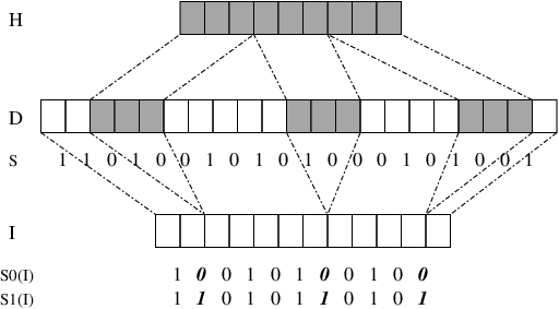
We concatenate fragments in $I$ and keep the $I$-internal separating variables as in $\mathbf{s}$. There are two variants of the segmentation for $I$, depending on how we define the separating variables between the fragments. So we have the following two segmented sub-sets.

• •

  $I_{\mathbf{s}_{0}(I)}$: inter-fragment separating variable = 0.

• •

  $I_{\mathbf{s}_{1}(I)}$: inter-fragment separating variable = 1.

Here, $\mathbf{s}_{0}(I)$ and $\mathbf{s}_{1}(I)$ represent the two segmentation vectors on $I$ respectively, each of which has $|I|-m_{j}-1$ changeable separating variables, where $|I|$ is the number words contained in $I$. The number of changeable variables that set to $1$ follows a binomial distribution $B(|I|-m_{j}-1,1-q)$. In Figure 3, fixed inter-fragment separating variables are represented in the bold italic font.

If there are $s$ changeable variables set to $1$ in $I_{\mathbf{s}_{0}(I)}$, the number of tokens in $I_{\mathbf{s}_{0}(I)}$ is $|I_{\mathbf{s}_{0}(I)}|=s+1$. Similarly, if there are $s$ changeable variables set to $1$ in $I_{\mathbf{s}_{1}(I)}$, the number of tokens in $I_{\mathbf{s}_{1}(I)}$ is $|I_{\mathbf{s}_{1}(I)}|=s+m_{j}+1$.

In addition, it is easy to verify that

	$\displaystyle|I_{\mathbf{s}_{0}(I)}|$	$\displaystyle\leq$	$\displaystyle|D_{\mathbf{s}}|$		(6)
	$\displaystyle|D_{\mathbf{s}}|$	$\displaystyle\leq$	$\displaystyle|I_{\mathbf{s}_{1}(I)}|+|u_{j}|m_{j}$		(7)

Combining (5), (6) and the two assumptions, we have the upper bound in Lemma 4.

Similarly, combining (5), (7) and the two assumptions, we obtain the lower bound in Lemma 5.

The proofs of Lemmas 4 and 5 are given in the Appendixes A and B respectively. The proof of Lemma 4 also depends on Lemma 8. Lemma 8 and its proof are given in Appendix C.

Therefore, Theorem 2 holds.

Theorem 2 is for joint distribution of token pairs. In previous work of using EPL, conditional probabilities were ofter used, for example, like $P(u|v)$ and $P(v|u)$. Starting from Theorem 2, we can easily obtain the following corollaries for conditional probabilities.

Proof According to the definition, $Pr(u,v_{j}|G_{D,d})=0$ and $L_{q}(u,v_{j})=0$, if $|u|\neq|v_{j}|$. Therefore, we only need to consider all pairs of $(u,v_{j})$, such that $|u|=|v_{j}|=|u_{j}|$. The number of distinct $u$ is a finite number, since source vocabulary is a finite set. Therefore, according to Theorem 2, for any small positive number $\epsilon$, there exists a positive number $n$, such that, if $|D|>n$, we have

$\displaystyle(1-\epsilon)\frac{L_{q}(u,v_{j})}{q^{|u_{j}|}}\leq Pr(u,v_{j}|G_{D,d})\leq(1+\epsilon)\frac{L_{q}(u,v_{j})}{q^{|u_{j}|}}$

(8)

Therefore, we have

	$\displaystyle Pr(u_{j}|v_{j},G_{D,d})$	$\displaystyle=$	$\displaystyle\frac{Pr(u_{j},v_{j}|G_{D,d})}{\sum_{u:|u|=|u_{j}|}Pr(u,v_{j}|G_{D,d})}$
		$\displaystyle\leq$	$\displaystyle\frac{(1+\epsilon)L_{q}(u,v_{j})/q^{|u_{j}|}}{\sum_{u:|u|=|u_{j}|}(1-\epsilon)L_{q}(u,v_{j})/q^{|u_{j}|}}\mbox{ \lx@text@lbrace Eqn. (\ref{eqn:conb})\lx@text@rbrace}$
		$\displaystyle=$	$\displaystyle\frac{1+\epsilon}{1-\epsilon}\frac{L_{q}(u_{j},v_{j})}{\sum_{u}L_{q}(u,v_{j})}$

Thus,

$\displaystyle Pr(u_{j}|v_{j},G_{D,d})/\frac{L_{q}(u_{j},v_{j})}{\sum_{u}L_{q}(u,v_{j})}$

$\displaystyle\leq$

$\displaystyle\frac{1+\epsilon}{1-\epsilon}$

Similarly, we have

$\displaystyle Pr(u_{j}|v_{j},G_{D,d})/\frac{L_{q}(u_{j},v_{j})}{\sum_{u}L_{q}(u,v_{j})}$

$\displaystyle\geq$

$\displaystyle\frac{1-\epsilon}{1+\epsilon}$

Therefore,

$$\lim_{|D|\to\infty}Pr(u_{j}|v_{j},G_{D,d})/\frac{L_{q}(u_{j},v_{j})}{\sum_{u}L_{q}(u,v_{j})}=1$$

The proof of Corollary 7 is similar to that of Corollary 6. Therefore, conditional probabilities in EPL are reasonable approximation of the conditional ensemble probability functions.

The proofs for the conditional probabilities depend on a special property of monotonic translation; the length of $u_{j}$ is the same as the length of $v_{j}$. However, this is not true in real application of phrase-based translation. The source and the target sides may have different segmentations. We leave the modeling of real phrase-based translation for future work.

Now we try to extend Theorem 2 to the string-to-tree grammar. First, we define a prior distribution on tree segmentation. We assign a Bernoulli variable to each tree node, representing the probabilities that we separate the tree at this node, i.e, with probabilities of $1-q$, we choose to separate each node.

Let $(u_{j},v_{j})$ be a string–tree pair, where $u_{j}$ is a source string and $v_{j}$ is a target tree. Let $t_{j}$ be the number of words in $u_{j}$, and let $n_{j}$ be the number of non-terminals in $u_{j}$, where $t_{j}+n_{j}\leq d$, and $\sum t_{j}$ is the length of the input sentence, $|\mathbf{x}|$. Thus, the probability that an appearance of $(u_{j},v_{j})$ in $D$ is exactly tokenized as in this way is $q^{t_{j}-1}(1-q)^{n_{j}+1}$.

With similar methods used in the proofs for string structures, we can show that, if Assumptions 1 and 2 hold,

$\displaystyle\lim_{|D|\to\infty}\frac{L_{q}(u_{j},v_{j})}{Pr(u_{j},v_{j}|G_{D,d})}$

$\displaystyle=$

$\displaystyle c\,q^{t_{j}-1}(1-q)^{n_{j}},$

where $c=\sum_{i:\,t_{i}+n_{i}\leq d}\#(u_{i},v_{i})/|D|$ is a constant, and $q$ is a free parameter. We skip the proof here to avoid duplication of similar procedure. We define

$\displaystyle P_{q,d}(u_{j},v_{j})$

$\displaystyle=$

$\displaystyle c\,q^{t_{j}-1}(1-q)^{n_{j}}Pr(u_{j},v_{j}|G_{D,d}).$

Thus, $P_{q,d}(u_{j},v_{j})$ approximates $L_{q}(u_{j},v_{j})$, where

$\displaystyle\lim_{|D|\to\infty}\frac{L_{q}(u_{j},v_{j})}{P_{q,d}(u_{j},v_{j})}=1.$

This result shows a theoretically better way of using heuristic grammar in string-to-tree models.

In the proofs of Lemmas 4 and 5, Assumption 2 is only used in the very last steps. Therefore, we could build the upper and lowers bounds of the ratio without Assumption 2 by connecting Inequalities (12) and (13) in Appendixes A and B respectively.

The ensemble probability in (4) can be viewed as simplification of a Bayesian model in (9).

	$\displaystyle L(u_{j},v_{j})$	$\displaystyle=$	$\displaystyle Pr(u_{j},v_{j}|D)$		(9)
		$\displaystyle=$	$\displaystyle\sum_{G\in\mathcal{G}(D)}Pr(u_{j},v_{j}|G)Pr(G|D)$

In (9), we marginalize all possible token-based grammars $G$ from $D$, $\mathcal{G}(D)$. Furthermore,

$\displaystyle Pr(G|D)$

$\displaystyle=$

$\displaystyle\sum_{\mathbf{s}}Pr(G|D,\mathbf{s})Pr(\mathbf{s}|D)$

Then, we approximate the posterior probability of $G$ given $D$ and $\mathbf{s}$ with point estimation. Thus, $Pr(G|D,\mathbf{s})=1$ if and only if $G$ is the MLE grammar of $D\mathbf{s}$, which means all the distribution mass is assigned to $G_{D\mathbf{s}}$, the MLE grammar for $D\mathbf{s}$. We also assume that $\mathbf{s}$ is independent of $D$. Thus,

$\displaystyle Pr(G|D)$

$\displaystyle=$

$\displaystyle\sum_{\mathbf{s}}\mathbf{1}(G=G_{D\mathbf{s}})Pr(\mathbf{s}),$

(10)

where $Pr(\mathbf{s})$ is a prior distribution of segmentation for any string of $|D|$ words. With (10), we can rewrite (9) as follows.

	$\displaystyle L(u_{j},v_{j})$	$\displaystyle=$	$\displaystyle\sum_{G\in\mathcal{G}(D)}Pr(u_{j},v_{j}|G)\sum_{\mathbf{s}}\mathbf{1}(G=G_{D\mathbf{s}})Pr(\mathbf{s})$		(11)
		$\displaystyle=$	$\displaystyle\sum_{\mathbf{s}}\sum_{G\in\mathcal{G}(D)}Pr(u_{j},v_{j}|G)\mathbf{1}(G=G_{D\mathbf{s}})Pr(\mathbf{s})$
		$\displaystyle=$	$\displaystyle\sum_{\mathbf{s}}Pr(u_{j},v_{j}|G_{{D\mathbf{s}}})Pr(\mathbf{s})$

Equation (11) is exactly the ensemble probability in Equation (4).

The EPL method investigated in this article may date back to Data Oriented Parsing (DOP) by Bod (1992). What is special with DOP is that the DOP model uses overlapping treelets of various sizes in an exhaustive way as building blocks of a statistical tree grammar.

In our framework, for each pair $(u_{j},v_{j})$, we can use $u_{j}$ to represent the input text, and $v_{j}$ to represent its tree structure. Thus, it would be similar to the string-to-tree model in Section 3.5. Joint probability of $(u_{j},v_{j})$ stands for unigram probability $Pr(\mbox{treelet})$.

However, the original DOP estimator (DOP1) is quite different from our monotonic translation model. The conditional probability in DOP1 is defined as $Pr(\mbox{treelet}|\mbox{subroot-label})$, so that there is no obvious way to model DOP1 with monotonic translation. Therefore, theoretical justification of DOP1 is still an open problem.

References

- Blunsom et al. (2009) Phil Blunsom, Trevor Cohn, Chris Dyer, and Miles Osborne. A gibbs sampler for phrasal synchronous grammar induction. In Proceedings of the 47th Annual Meeting of the Association for Computational Linguistics (ACL), pages 782–790, Suntec, Singapore, August 2009.
- Bod (1992) Rens Bod. A computational model of language performance: Data Oriented Parsing. In Proc. of COLING92, 1992.
- Carreras and Collins (2009) Xavier Carreras and Michael Collins. Non-projective parsing for statistical machine translation. In Proceedings of the 2009 Conference of Empirical Methods in Natural Language Processing, pages 200–209, Singapore, 2009.
- Chiang (2005) David Chiang. A hierarchical phrase-based model for statistical machine translation. In Proceedings of the 43th Annual Meeting of the Association for Computational Linguistics (ACL), pages 263–270, Ann Arbor, MI, 2005.
- Cohn and Blunsom (2009) Trevor Cohn and Phil Blunsom. A Bayesian model of syntax-directed tree to string grammar induction. In Proceedings of the 2009 Conference of Empirical Methods in Natural Language Processing, pages 352–361, Singapore, August 2009.
- Cohn et al. (2009) Trevor Cohn, Sharon Goldwater, and Phil Blunsom. Inducing compact but accurate tree-substitution grammars. In Proceedings of the 2009 Human Language Technology Conference of the North American Chapter of the Association for Computational Linguistics, pages 548–556, Boulder, Colorado, June 2009.
- Daumé III (2008) Hal Daumé III. Natural language processing blog: Teaching machine translation. http://nlpers.blogspot.com/2008/05/teaching-machine-translation.html, 2008.
- Daumé III and Marcu (2005) Hal Daumé III and Daniel Marcu. Learning as search optimization: Approximate large margin methods for structured prediction. In Proceedings of the 22nd International Conference on Machine Learning, 2005.
- DeNero et al. (2006) John DeNero, Dan Gillick, James Zhang, and Dan Klein. Why generative phrase models underperform surface heuristics. In Proceedings of the Workshop on Statistical Machine Translation, 2006.
- DeNero et al. (2008) John DeNero, Alexandre Bouchard-Côté, and Dan Klein. Sampling alignment structure under a Bayesian translation model. In Proceedings of the 2008 Conference of Empirical Methods in Natural Language Processing, 2008.
- Galley et al. (2006) Michel Galley, Jonathan Graehl, Kevin Knight, Daniel Marcu, Steve DeNeefe, Wei Wang, and Ignacio Thayer. Scalable inference and training of context-rich syntactic models. In COLING-ACL ’06: Proceedings of 44th Annual Meeting of the Association for Computational Linguistics and 21st Int. Conf. on Computational Linguistics, pages 961–968, Sydney, Australia, 2006.
- Johnson (2002) Mark Johnson. The DOP estimation method is biased and inconsistent. Computational Linguistics, 28(1), 2002.
- Koehn et al. (2003) Philipp Koehn, Franz J. Och, and Daniel Marcu. Statistical phrase based translation. In Proceedings of the 2003 Human Language Technology Conference of the North American Chapter of the Association for Computational Linguistics, pages 48–54, Edmonton, Canada, 2003.
- Och and Ney (2004) Franz J. Och and Hermann Ney. The alignment template approach to statistical machine translation. Computational Linguistics, 30(4), 2004.
- Post and Gildea (2009) Matt Post and Daniel Gildea. Bayesian learning of a tree substitution grammar. In Proceedings of the 47th Annual Meeting of the Association for Computational Linguistics (ACL), pages 45–48, Suntec, Singapore, August 2009.
- Prescher et al. (2004) Detlef Prescher, Remko Scha, Khalil Sima’an, and Andreas Zollmann. On the statistical consistency of dop estimators. In Proceedings of the 14th Meeting of Computational Linguistics in the Netherlands, 2004.
- Quirk et al. (2005) Chris Quirk, Arul Menezes, and Colin Cherry. Dependency treelet translation: Syntactically informed phrasal SMT. In Proceedings of the 43th Annual Meeting of the Association for Computational Linguistics (ACL), pages 271–279, Ann Arbor, MI, 2005.
- Shen et al. (2008) Libin Shen, Jinxi Xu, and Ralph Weischedel. A new string-to-dependency machine translation algorithm with a target dependency language model. In Proceedings of the 46th Annual Meeting of the Association for Computational Linguistics (ACL), 2008.
- Zettlemoyer and Collins (2005) Luke Zettlemoyer and Michael Collins. Learning to map sentences to logical form: Structured classification with probabilistic categorial grammars. 2005.