跳到论文正文
W Papers独立论文阅读器 arXiv:1104.3911 论文正文 计算阅读时间 · 0%
引用这篇论文根据当前论文元数据生成,正式投稿前建议核对。


License: arXiv.org perpetual non-exclusive license
arXiv:1104.3911v2 [cs.IT] 21 Apr 2011

Information Exchange Limits in Cooperative MIMO Networks

Ali Tajer ††thanks: Electrical Engineering Department, Princeton University, Princeton, NJ 08540 (email: tajer@princeton.edu).    Xiaodong Wang ††thanks: Electrical Engineering Department, Columbia University, New York, NY 10027 (email: wangx@ee.columbia.edu).
Abstract

Concurrent presence of inter-cell and intra-cell interferences constitutes a major impediment to reliable downlink transmission in multi-cell multiuser networks. Harnessing such interferences largely hinges on two levels of information exchange in the network: one from the users to the base-stations (feedback) and the other one among the base-stations (cooperation). We demonstrate that exchanging a finite number of bits across the network, in the form of feedback and cooperation, is adequate for achieving the optimal capacity scaling. We also show that the average level of information exchange is independent of the number of users in the network. This level of information exchange is considerably less than that required by the existing coordination strategies which necessitate exchanging infinite bits across the network for achieving the optimal sum-rate capacity scaling. The results provided rely on a constructive proof.

1 Introduction

Multiple-antenna broadcast transmission is known to offer substantial improvement in spectral efficiency via spatial multiplexing. Such gains depend heavily on the availability of some channel state information (CSI) at the transmitter. Acquiring such CSI allows for managing the intra-cell interference which is due to spatial multiplexing. There exists a rich literature on the design of user scheduling that spans a wide range of transceiver designs with different levels of complexity and CSI feedback requirements [1, 2, 3].

In multi-cell multiuser networks, besides the intra-cell interference caused by the residual interference remaining after spatial multiplexing within each cell, another impediment arises from inter-cell interference due to the ever-shrinking cell sizes, which makes the networks operate in interference-limited, rather than noise-limited, regimes. Alleviating the effects of inter-cell interference requires the base-stations to cooperatively adjust their transmissions [4, 5, 6, 7]. Coordination among the base-stations for downlink transmission imposes some information exchange (cooperation) among the base-stations. Once full CSI feedback and full cooperation is viable, i.e., all the users report their CSI to all base-stations, and all base-stations share their information streams, the multi-cell network can be essentially modeled as a single-cell multiple-input multiple-output (MIMO) broadcast channel with a transmit antenna array of a higher dimension. Using the literature on MIMO broadcast channel immediately establishes the optimal sum-rate capacity scaling of multi-cell multiuser networks which is achievable via dirty-paper coding [3].

Such optimal capacity scaling, however, necessitates full feedback and cooperation across the network. This requirement, specially in large networks, can potentially overburden the feedback channels as well as the backbone channels that connect the base-stations. Therefore, it becomes imperative to study whether such full information exchange is all necessary or contains some redundancy that can be avoided. The question we are specifically trying to address is: what is the minimum amount of information exchange, in the form of either CSI feedback or base-station cooperation, that ensures retaining the optimal sum-rate capacity scaling?

We consider a multi-cell network model, in which every few neighboring cells are collectively regarded as a super-cell that serve the users within that super-cell collaboratively. The analysis demonstrates that for the purpose of achieving the optimal scaling, cooperation among the super-cells, while desirable, is not necessary. In other words, while collective transmission by the base-stations across the super-cells has certain advantages, as long as achieving the optimal capacity scaling is concerned, the super-cells can decide about their scheduling policies independently. Furthermore, each user has to provide feedback to only the base-stations of its designated super-cell. These two relaxations essentially imply that base-stations of each super-cell collect only local information and any information exchange across super-cells are avoided. We also quantify the aggregate amount of information exchange necessary for achieving the optimal sum-rate capacity scaling. Specifically, we show that when the network contains MM super-cells, each consisting of QQ base-stations and when each base-station is equipped with NtN_{t} transmit antennas, the minimum aggregate amount of information exchange in the network to guarantee optimal capacity scaling is upper bounded by M​Q​Nt​⌈log⁡Q​Nt⌉MQN_{t}\lceil\log QN_{t}\rceil, which is independent of the number of users in the network.

These results in this paper are provided through a constructive proof. The flow of the proof is as follows. After discussing the network model in Section 2 we describe a scheduling procedure and feedback mechanism in Section 3. Next, in Section 4 we show that proposed scheduler yields the optimal sum-rate capacity scaling. Then in Section 5 we assess the aggregate amount of information exchange that the proposed scheduler requires. Section 6 addresses some practical issues, e.g., the impact of the size of the super-cells and fairness, and finally Section 7 concludes the paper. To enhance the flow of the content, most of the proofs are relegated in the appendices.

We remark that as opposed to multi-cell MIMO networks, there exists a rich literature on single-cell downlink transmission that investigate the interplay between the feedback load and broadcast sum-rate throughput scaling. One group of studies, c.f. [8, 9, 10], for single-cell systems consider feeding back unquantized real values (channel magnitude or 𝖲𝖭𝖱{\sf SNR}, which in theory requires infinite-rate feedback. In another line of studies, c.f., [11], finite-rate feedback mechanisms are introduced. However, the optimal sum-rate throughput is achievable in these studies when the number of feedback bits tends to infinity. The proposed feedback mechanisms in [12, 13], impose only finite-rate feedback loads and achieve the optimal multiuser diversity gain. However, since they do not allow for simultaneous transmissions to multiple users, they cannot capture the multiplexing gain. Finally, the heuristic feedback mechanisms proposed in [14, 15] have limited feedback loads for which the sum-rate throughput scaling analysis is not provided. As a by-product of our analysis we find that in a single-cell downlink transmission it is possible to achieve the optimal capacity scaling rate with finite-rate feedback. It is also noteworthy on a different research direction, that capacity scaling for some infrastructure-based sensor networks are provided in [16], [17]

2 System Model

Consider the downlink transmission in a MIMO network that consists of MM super-cells, each comprising of QQ regular cells equipped with one base-station. We use the shorthand 𝒬m{\cal Q}_{m} to refer to the mt​hm^{th} super-cell and denote its base-stations by Bmr,B^{r}_{m}, for r∈{1,…,Q}r\in\{1,\dots,Q\}. Let KK denote the number of users per super-cell and assume that the base-stations of each super-cell accomplish the downlink transmissions collaboratively. Moreover, we assume that all the base-stations within a super-cell are fully cooperative, i.e., are connected through a backbone link that allows them to share their information streams and to carry out fully coordinated downlink transmissions. The case that such cooperation is not viable corresponds to the setting Q=1Q=1. We also use the shorthand UnkU^{k}_{n} to denote the kt​hk^{th} user in the nt​hn^{th} super-cell, respectively, for k∈{1,…,K}k\in\{1,\dots,K\} and n∈{1,…,M}n\in\{1,\dots,M\}.

Define 𝑯n,mk,r∈ℂNr×Nt{\boldsymbol{H}}_{n,m}^{k,r}\in\mathbb{C}^{N_{r}\times N_{t}} as the downlink channel from base-station BmrB^{r}_{m} to user UnkU^{k}_{n} and let 𝒙mr​(t)∈ℂNt×1{\boldsymbol{x}}^{r}_{m}(t)\in\mathbb{C}^{N_{t}\times 1} denote the signal vector transmitted by base-station BmrB^{r}_{m} at time instance tt. The received signal by UnkU^{k}_{n} at time instance tt is therefore given by

𝒚nk​(t)=∑m=1M∑r=1Qγn,mk,r​𝑯n,mk,r​𝒙mr​(t)+𝒛nk​(t),{\boldsymbol{y}}^{k}_{n}(t)=\sum_{m=1}^{M}\sum_{r=1}^{Q}\sqrt{\gamma^{k,r}_{n,m}}\ {\boldsymbol{H}}^{k,r}_{n,m}{\boldsymbol{x}}^{r}_{m}(t)+{\boldsymbol{z}}^{k}_{n}(t)\ ,

where γn,mk,r∈ℝ+\gamma^{k,r}_{n,m}\in\mathbb{R}^{+} is incorporated to capitalize the combined effect of transmission power and signal attenuation (path-loss) between BmrB^{r}_{m} and UnkU^{k}_{n}. In non-homogenous networks the terms {γn,mk,r}\{\gamma^{k,r}_{n,m}\} are distinct as different users undergo different path-loss and shadowing effects. Also, 𝒛nk∈ℂNr×1{\boldsymbol{z}}^{k}_{n}\in\mathbb{C}^{N_{r}\times 1} accounts for the additive white Gaussian noise distributed as 𝒞​𝒩​(𝟎,𝑰Nr)\mathcal{CN}(\boldsymbol{0},{\boldsymbol{I}}_{N_{r}}). We consider block frequency-flat fading channels and assume that the entries of the channel matrix 𝑯n,mk,r{\boldsymbol{H}}^{k,r}_{n,m} are independent and identically distributed as complex Gaussian 𝒞​𝒩​(0,1)\mathcal{CN}(0,1). In order to facilitate spatial multiplexing and to harness its ensuing interference as well as the inter-cell interference, the base-stations employ linear precoding. We define {𝝎mr​(ℓ)}ℓ=1Nt\{\boldsymbol{\omega}^{r}_{m}(\ell)\}_{\ell=1}^{N_{t}} as the set of linear precoders employed by base-station BmrB^{r}_{m}. By further defining xmr​(ℓ,t)x^{r}_{m}(\ell,t) as the information symbol that BmrB^{r}_{m} transmits along the beamforming vector 𝝎mr​(ℓ)\boldsymbol{\omega}^{r}_{m}(\ell), at any time instance tt we have

𝒙mr​(t)=∑ℓ=1Ntxmr​(ℓ,t)​𝝎mr​(ℓ).{\boldsymbol{x}}^{r}_{m}(t)=\sum_{\ell=1}^{N_{t}}x^{r}_{m}(\ell,t)\;\boldsymbol{\omega}^{r}_{m}(\ell)\ . (1)

Motivated by refraining from information feedback about channel directions the base-stations exploit the notion of orthogonal random beamforming first proposed in [8]. For this purpose, at the beginning of each block transmission, each base-station generates NtN_{t} orthonormal vectors {𝝎mr​(ℓ)}ℓ=1Nt\{\boldsymbol{\omega}^{r}_{m}(\ell)\}_{\ell=1}^{N_{t}}, according to an isotropic distribution [18]. The user UnkU^{k}_{n} knows 𝑯n,nk,r​𝝎nr​(ℓ){\boldsymbol{H}}^{k,r}_{n,n}\boldsymbol{\omega}^{r}_{n}(\ell) for ℓ∈{1,…,Nt}\ell\in\{1,\dots,N_{t}\} and r∈{1,…,Q}r\in\{1,\dots,Q\} perfectly and instantaneously. We denote the transmission power per information stream by ρ=△PNt\rho\stackrel{{\scriptstyle\scriptscriptstyle\triangle}}{{=}}\frac{P}{N_{t}}, where PP is the average power per base-station. Also, throughout the paper, we use the convention aK≐bKa_{K}\doteq b_{K} to denote asymptotic equality, i.e., limK→∞aKbK=1\lim_{K\rightarrow\infty}\frac{a_{K}}{b_{K}}=1. Operators ≤⋅{\overset{\cdot}{\leq}} and ≥⋅{\overset{\cdot}{\geq}} are defined accordingly. All the logarithms, unless otherwise mentioned, are in base 2 and throughput are in bits/sec/Hz.

3 Scheduling Framework

We first consider the case that the users have one receive antenna and will later generalize it the case of arbitrary number of receive antennas in Section 4. We assume that the users employ single-user decoders such that all the inter-cell and intra-cell interferers are treated as Gaussian noise. While more advanced receivers will offer better performance, we show that the simple single-user decoders are sufficient to fully capture the optimal multiplexing and multiuser diversity gains in MIMO networks.

Due to full cooperation, the information stream that some base-station in the super-cell 𝒬n{\cal Q}_{n} intends to transmit to user UnkU^{k}_{n} is known to all base-stations of that super-cell. Therefore, the message intended for user UnkU^{k}_{n} can be transmitted along any arbitrary beamforming vector of any base-station of 𝒬n{\cal Q}_{n}. Hence, user UnkU^{k}_{n} can compute the following Q×NtQ\times N_{t} distinct 𝖲𝖨𝖭𝖱{\sf SINR}s given that its intended information is embedded in xnr​(ℓ,t)x^{r}_{n}(\ell,t) and transmitted by the base-station BmrB^{r}_{m} along 𝝎nr​(ℓ)\boldsymbol{\omega}^{r}_{n}(\ell), where r∈{1,…,Q}r\in\{1,\dots,Q\} and ℓ∈{1,…,Nt}\ell\in\{1,\dots,N_{t}\},

𝖲𝖨𝖭𝖱nk​(r,ℓ)=γn,nk,r​|𝑯n,nk,r​𝝎nr​(ℓ)|2∑m=1M∑r′=1Qγn,mk,r′​∑ℓ′=1Nt|𝑯n,mk,r′​𝝎mr′​(ℓ′)|2−γn,nk,r​|𝑯n,nk,r​𝝎nr​(ℓ)|2+1ρ.\displaystyle{\sf SINR}^{k}_{n}(r,\ell)=\frac{\gamma_{n,n}^{k,r}|{\boldsymbol{H}}^{k,r}_{n,n}\boldsymbol{\omega}^{r}_{n}(\ell)|^{2}}{\sum_{m=1}^{M}\sum_{r^{\prime}=1}^{Q}\gamma^{k,r^{\prime}}_{n,m}\sum_{\ell^{\prime}=1}^{N_{t}}|{\boldsymbol{H}}^{k,r^{\prime}}_{n,m}\boldsymbol{\omega}^{r^{\prime}}_{m}(\ell^{\prime})|^{2}-\gamma_{n,n}^{k,r}|{\boldsymbol{H}}^{k,r}_{n,n}\boldsymbol{\omega}^{r}_{n}(\ell)|^{2}+\frac{1}{\rho}}\ . (2)

It can be readily verified that for any given ℓ\ell and for any (k,n,r)≠(k′,n′,r′)(k,n,r)\neq(k^{\prime},n^{\prime},r^{\prime}), the numerators and denumerators of 𝖲𝖨𝖭𝖱nk​(r,ℓ){\sf SINR}^{k}_{n}(r,\ell) and 𝖲𝖨𝖭𝖱n′k′​(r′,ℓ){\sf SINR}^{k^{\prime}}_{n^{\prime}}(r^{\prime},\ell) are disjoint. In other words, any term of the form 𝑯n,mk,r​𝝎nr​(ℓ){\boldsymbol{H}}^{k,r}_{n,m}\boldsymbol{\omega}^{r}_{n}(\ell) that appears in the characterization of 𝖲𝖨𝖭𝖱nk​(r,ℓ){\sf SINR}^{k}_{n}(r,\ell) does not appear in that of 𝖲𝖨𝖭𝖱n′k′​(r′,ℓ){\sf SINR}^{k^{\prime}}_{n^{\prime}}(r^{\prime},\ell). By invoking the statistical independence of the channel coefficients and beamforming vectors, we find that 𝖲𝖨𝖭𝖱nk​(r,ℓ){\sf SINR}^{k}_{n}(r,\ell) and 𝖲𝖨𝖭𝖱n′k′​(r′,ℓ){\sf SINR}^{k^{\prime}}_{n^{\prime}}(r^{\prime},\ell) are also statistically independent for any (k,n,r)≠(k′,n′,r′)(k,n,r)\neq(k^{\prime},n^{\prime},r^{\prime}). However, by noting the different attenuation factors {γn,mk,r}\{\gamma^{k,r}_{n,m}\} for different choices of k,n,rk,n,r, 𝖲𝖨𝖭𝖱nk​(r,ℓ){\sf SINR}^{k}_{n}(r,\ell) and 𝖲𝖨𝖭𝖱n′k′​(r′,ℓ){\sf SINR}^{k^{\prime}}_{n^{\prime}}(r^{\prime},\ell) are not identically distributed. Similarly it can be shown that for any fixed set of k,n,rk,n,r the terms {𝖲𝖨𝖭𝖱nk​(r,ℓ)}\{{\sf SINR}^{k}_{n}(r,\ell)\} are statistically identical but not independent. We denote the cumulative distribution function (CDF) of 𝖲𝖨𝖭𝖱nk​(r,ℓ){\sf SINR}^{k}_{n}(r,\ell) for ℓ∈{1,…,Nt}\ell\in\{1,\dots,N_{t}\} by

Fnk​(x,r):ℝ+→[0,1].F^{k}_{n}(x;r):\mathbb{R}_{+}\rightarrow[0,1]\ .

We propose a user scheduling procedure that aims at identifying and serving Q​NtQN_{t} users in each super-cell such that 1) the network sum-rate throughput captures the full multiuser diversity gain, 2) does not impose any information exchange or cooperation among the super-cells, and 3) necessitates each base-station to acquire only a finite number of feedback bits from each of its designated users. The steps involved in the proposed scheduling procedure are summarized as follows. We remark that the notion of random beamforming, first deployed in [8], has been the core of many scheduling schemes for single-cell broadcast channels.

1) Normalizing 𝖲𝖨𝖭𝖱{\sf SINR}s:

For each user UnkU^{k}_{n} we define QQ positive scalars {βnk​(1),…,βnk​(Q)}\{\beta^{k}_{n}(1),\dots,\beta^{k}_{n}(Q)\} each pertaining to one of the base-station of the super-cell 𝒬n{\cal Q}_{n}.

∀r∈{1,…,Q}:defineβnk(r)such thatFnk(βnk(r);r)=1−1K.\forall r\in\{1,\dots,Q\}:\quad\mbox{define}\quad\beta^{k}_{n}(r)\;\;\mbox{such that}\;\;F^{k}_{n}\big(\beta^{k}_{n}(r);r\big)=1-\frac{1}{K}\ . (3)

There exist unique solutions for βnk​(r)\beta^{k}_{n}(r) as Fnk​(x,r)F^{k}_{n}(x;r) is a CDF and strictly monotonic in xx. Next, corresponding to each user UnkU^{k}_{n} we define the following normalized 𝖲𝖨𝖭𝖱{\sf SINR} terms.

𝗌𝗂𝗇𝗋nk(r,ℓ)=△𝖲𝖨𝖭𝖱nk​(r,ℓ)βnk​(r),∀r∈{1,…,Q}andℓ∈{1,…,Nt}.{\sf sinr}^{k}_{n}(r,\ell)\stackrel{{\scriptstyle\scriptscriptstyle\triangle}}{{=}}\frac{{\sf SINR}^{k}_{n}(r,\ell)}{\beta^{k}_{n}(r)}\ ,\quad\forall r\in\{1,\dots,Q\}\quad\mbox{and}\quad\ell\in\{1,\dots,N_{t}\}\ . (4)
2) Feedback:

a

  1. 1.

    Recall that each user UnkU^{k}_{n} can be served along any beamformer of the super-cell 𝒬n{\cal Q}_{n}. Among all beamformers, we identify the most favorable beam for the user UnkU^{k}_{n}, that is the beamformer yielding the highest 𝖲𝖨𝖭𝖱{\sf SINR} for UnkU^{k}_{n}, i.e.,

    𝗌𝗂𝗇¯​𝗋𝗇𝗄=△max𝗋,ℓ⁡𝗌𝗂𝗇𝗋𝗇𝗄​(𝗋,ℓ).\overline{\sf sin}{\sf r}^{k}_{n}\stackrel{{\scriptstyle\scriptscriptstyle\triangle}}{{=}}\max_{r,\;\ell}{\sf sinr}^{k}_{n}(r,\ell)\ . (5)
  2. 2.

    If 𝗌𝗂𝗇¯​𝗋𝗇𝗄≥𝟣\overline{\sf sin}{\sf r}^{k}_{n}\geq 1, then user UnkU^{k}_{n} feeds back the index of its most favorable beam to the base-stations of the super-cell 𝒬n{\cal Q}_{n}. As a super-cell has Q​NtQN_{t} beamformers, conveying such feedback requires ⌈log⁡Q​Nt⌉\lceil\log QN_{t}\rceil information bits.

3) User Selection:

a

  1. 1.

    Based on the information fed back by the users, corresponding to each super-cell 𝒬n{\cal Q}_{n} we construct the sets ℋnr​(ℓ){\cal H}^{r}_{n}(\ell), for r∈{1,…,Q}r\in\{1,\dots,Q\} and ℓ∈{1,…,Nt}\ell\in\{1,\dots,N_{t}\}, such that ℋnr​(ℓ){\cal H}^{r}_{n}(\ell) contains the indices of the users in 𝒬n{\cal Q}_{n} who have declared 𝝎nr​(ℓ)\boldsymbol{\omega}^{r}_{n}(\ell) as their most favorable beam. By invoking (5) we have

    ℋnr(ℓ)=△{k|𝗌𝗂𝗇¯𝗋𝗇𝗄≥𝟣and𝗌𝗂𝗇¯𝗋𝗇𝗄=𝗌𝗂𝗇𝗋𝗇𝗄(𝗋,ℓ)}.{\cal H}^{r}_{n}(\ell)\stackrel{{\scriptstyle\scriptscriptstyle\triangle}}{{=}}\Big\{k\;|\;\overline{\sf sin}{\sf r}^{k}_{n}\geq 1\quad\mbox{and}\quad\overline{\sf sin}{\sf r}^{k}_{n}={\sf sinr}^{k}_{n}(r,\ell)\Big\}\ . (6)
  2. 2.

    Super-cell 𝒬n{\cal Q}_{n} randomly selects one user from each set ℋnr​(ℓ){\cal H}^{r}_{n}(\ell) for r∈{1,…,Q}r\in\{1,\dots,Q\} and ℓ∈{1,…,Nt}\ell\in\{1,\dots,N_{t}\} and embeds the information signal intended for this user in the stream xnr​(ℓ)x^{r}_{n}(\ell). Note that the sets {ℋnr​(ℓ)}r,ℓ\{{\cal H}^{r}_{n}(\ell)\}_{r,\ell} are mutually disjoint and as a result, it is guaranteed that a user will not be served by more than one beam.

This procedure involves information exchange only in the form of feedback from the users to their designated base-stations and the super-cells do not cooperate or exchange any information. The crucial part of such scheduling is the appropriate design of the normalization factors βnk​(r)\beta^{k}_{n}(r) that results in a user selection yielding the optimal capacity scaling. The choices of the normalization factors as characterized in (3) serve a two-fold purpose, namely they control the aggregate amount of feedback and maintain fairness. As the network size KK increases, the normalization factors βnk​(r)\beta^{k}_{n}(r) as defined in (3) affect the feedback load in two ways. On one hand more users are competing for accessing the resources and it is expected that more users participate in the feedback process. On the other hand, as KK increases the normalization factors increase, which makes it harder for individual users in a network to satisfy the conditions for feeding back information to their designated base stations. As shown later in the paper, the combined impact of these two effects is in favor of reducing the feedback load. Also, as for the fairness, incorporating the statistics of the 𝖲𝖨𝖭𝖱{\sf SINR}s in the choices of the normalization factors ensures that all the users are equiprobable in satisfying their feedback constraint and consequently by invoking the selection procedure, all are equiprobable in having access to the resources. The proposed scheduling mechanism requires the users acquire the 𝖲𝖨𝖭𝖱{\sf SINR}s yielded by different beamformers. Such 𝖲𝖨𝖭𝖱{\sf SINR} acquisition can be accomplished during the training phase when the users obtain the channel states prior to the downlink transmission of data.

4 Throughput Scaling Analysis

When in a MIMO network perfect cooperation (full information exchange) among all super-cells is allowed, it can be effectively modeled as a large single-cell multiple-antenna broadcast channel with M​Q​NtMQN_{t} transmit antennas and M​KMK users. In  [3, 8] it shown that for such downlink transmission the sum-rate capacity, which is achievable via dirty-paper coding, scales with increasing KK as

𝔼𝑯​[R]≐M​Q​Nt​log⁡log⁡K​Nr.\mathbb{E}_{\boldsymbol{H}}[R]\doteq MQN_{t}\log\log KN_{r}\ . (7)

In the sequel we analyze the sum-rate throughput scaling of our proposed procedure and demonstrate that the achievable throughput scales similar to (7).

4.1 Throughput Scaling for Nr=1N_{r}=1

By defining RnR_{n} as the sum-rate throughput achieved for the nt​hn^{th} super-cell, the expected sum-rate throughput of the network is 𝔼𝑯​[R]=∑n=1M𝔼𝑯​[Rn]\mathbb{E}_{\boldsymbol{H}}[R]=\sum_{n=1}^{M}\mathbb{E}_{\boldsymbol{H}}[R_{n}]. We further define Rnr​(ℓ)R^{r}_{n}(\ell) as the rate supported through the transmission along the beamforming vector 𝝎nr​(ℓ)\boldsymbol{\omega}^{r}_{n}(\ell). As formalized in (6), the super-cell 𝒬n{\cal Q}_{n} constructs the new set ℋ¯n\bar{\cal H}_{n}, as the set of the user index sets ℋnr​(ℓ){\cal H}^{r}_{n}(\ell) for all rr and ℓ\ell, i.e., ℋ¯n=△{ℋnr​(ℓ)}r,ℓ\bar{\cal H}_{n}\stackrel{{\scriptstyle\scriptscriptstyle\triangle}}{{=}}\{{\cal H}^{r}_{n}(\ell)\}_{r,\ell}. Conditioned on the sets ℋ¯n\bar{\cal H}_{n}, the sum-rate throughput supported in the nt​hn^{th} super-cell is the summation of the rates its individual beamformers can sustain. Therefore,

𝔼𝑯​[Rn|ℋ¯n]=∑r=1Q∑ℓ=1Nt𝔼𝑯​[Rnr​(ℓ)|ℋnr​(ℓ)].\mathbb{E}_{\boldsymbol{H}}[R_{n}\;|\;\bar{\cal H}_{n}]=\sum_{r=1}^{Q}\sum_{\ell=1}^{N_{t}}\mathbb{E}_{\boldsymbol{H}}[R^{r}_{n}(\ell)\;|\;{\cal H}^{r}_{n}(\ell)]\ . (8)

As designated by the user scheduling procedure, for each r∈{1,…,Q}r\in\{1,\dots,Q\} and ℓ∈{1,…,Nt}\ell\in\{1,\dots,N_{t}\}, one of the members of the set ℋnr​(ℓ){\cal H}^{r}_{n}(\ell) is opted randomly to be served along the beamforming vector 𝝎nr​(ℓ)\boldsymbol{\omega}^{r}_{n}(\ell). Hence, each user with its index in ℋnr​(ℓ){\cal H}^{r}_{n}(\ell) will be selected to be served along the beamformer 𝝎nr​(ℓ)\boldsymbol{\omega}^{r}_{n}(\ell) with probability 1|ℋnr​(ℓ)|\frac{1}{|{\cal H}^{r}_{n}(\ell)|}. As a result given the set of candidate users ℋnr​(ℓ){\cal H}^{r}_{n}(\ell), the expected value of the rate sustained by the beamformer 𝝎nr​(ℓ)\boldsymbol{\omega}^{r}_{n}(\ell) is equal to the arithmetic average of the rates these candidate users can sustain. By noting that if the transmission of the beamformer 𝝎nt​(ℓ)\boldsymbol{\omega}^{t}_{n}(\ell) is intended for user UnkU^{k}_{n} then Rnr​(ℓ)=log⁡(1+𝖲𝖨𝖭𝖱nk​(r,ℓ))R^{r}_{n}(\ell)=\log(1+{\sf SINR}^{k}_{n}(r,\ell)), we obtain

𝔼𝑯​[Rnr​(ℓ)|ℋnr​(ℓ)]=1|ℋnr​(ℓ)|​∑k∈ℋnr​(ℓ)𝔼𝑯​[log⁡(1+𝖲𝖨𝖭𝖱nk​(r,ℓ))|ℋnr​(ℓ)].\displaystyle\mathbb{E}_{\boldsymbol{H}}[R^{r}_{n}(\ell)\;|\;{\cal H}^{r}_{n}(\ell)]=\frac{1}{|{\cal H}^{r}_{n}(\ell)|}\sum_{k\in{\cal H}^{r}_{n}(\ell)}\mathbb{E}_{\boldsymbol{H}}\left[\log\left(1+{\sf SINR}^{k}_{n}(r,\ell)\right)\;\big|\;{\cal H}^{r}_{n}(\ell)\right]. (9)

The next lemma, which provides a lower bound on 𝔼𝑯​[Rnr​(ℓ)|ℋnr​(ℓ)]\mathbb{E}_{\boldsymbol{H}}[R^{r}_{n}(\ell)\;|\;{\cal H}^{r}_{n}(\ell)] is instrumental to analyzing the scaling rate of 𝔼𝑯​[Rnr​(ℓ)|ℋnr​(ℓ)]\mathbb{E}_{\boldsymbol{H}}[R^{r}_{n}(\ell)\;|\;{\cal H}^{r}_{n}(\ell)].

Lemma 1 (Conditional Expected Rates)

If βnk​(r)≥1\beta^{k}_{n}(r)\geq 1 ∀n∈{1,…,M}\forall n\in\{1,\dots,M\}, ∀k∈{1,…,K}\forall k\in\{1,\dots,K\}, and ∀r∈{1,…,Q}\forall r\in\{1,\dots,Q\}, then

𝔼𝑯​[Rnr​(ℓ)|ℋnr​(ℓ)]≥ℛnr​(ℓ,|ℋnr​(ℓ)|)=△1|ℋnr​(ℓ)|​∑j=1|ℋnr​(ℓ)|𝔼𝑯​[log⁡(1+𝖲𝖨𝖭𝖱n(j)​(r,ℓ))],\displaystyle\mathbb{E}_{\boldsymbol{H}}[R^{r}_{n}(\ell)\;|\;{\cal H}^{r}_{n}(\ell)]\;\;\geq\;\;{\cal R}^{r}_{n}(\ell,|{\cal H}^{r}_{n}(\ell)|)\;\;\stackrel{{\scriptstyle\scriptscriptstyle\triangle}}{{=}}\;\;\frac{1}{|{\cal H}^{r}_{n}(\ell)|}\sum_{j=1}^{|{\cal H}^{r}_{n}(\ell)|}\mathbb{E}_{\boldsymbol{H}}\left[\log\left(1+{\sf SINR}^{(j)}_{n}(r,\ell)\right)\right]\ , (10)

where 𝖲𝖨𝖭𝖱n(j)​(r,ℓ){\sf SINR}^{(j)}_{n}(r,\ell) denotes the jt​hj^{th} largest element of the set {𝖲𝖨𝖭𝖱n1​(r,ℓ),…,𝖲𝖨𝖭𝖱nK​(r,ℓ)}\{{\sf SINR}^{1}_{n}(r,\ell),\dots,{\sf SINR}^{K}_{n}(r,\ell)\}.

Proof: See Appendix A.   

Equations (8) and (9) along with Lemma 1 (conditional expected rates) establish that if ∀k,n,r\forall k,n,r the normalizing factors satisfy the constraints βnk​(r)≥1\beta^{k}_{n}(r)\geq 1, then we have

𝔼𝑯​[Rn]\displaystyle\mathbb{E}_{\boldsymbol{H}}[R_{n}] =\displaystyle= ∑ℋ¯nP⁡(ℋ¯n)​𝔼𝑯​[Rn|ℋ¯n]\displaystyle\sum_{\bar{\cal H}_{n}}P(\bar{\cal H}_{n})\;\mathbb{E}_{\boldsymbol{H}}[R_{n}\;|\;\bar{\cal H}_{n}] (11)
=(8)\displaystyle\overset{\eqref{eq:Rm}}{=} ∑ℋ¯nP⁡(ℋ¯n)​∑r=1Q∑ℓ=1Nt𝔼𝑯​[Rnr​(ℓ)|ℋnr​(ℓ)]\displaystyle\sum_{\bar{\cal H}_{n}}P(\bar{\cal H}_{n})\sum_{r=1}^{Q}\sum_{\ell=1}^{N_{t}}\mathbb{E}_{\boldsymbol{H}}[R^{r}_{n}(\ell)\;|\;{\cal H}^{r}_{n}(\ell)]
≥(10)\displaystyle\overset{\eqref{eq:Rm_bound}}{\geq} ∑ℋ¯nP⁡(ℋ¯n)​∑r,ℓℛnr​(ℓ,|ℋnr​(ℓ)|).\displaystyle\sum_{\bar{\cal H}_{n}}P(\bar{\cal H}_{n})\sum_{r,\;\ell}{\cal R}^{r}_{n}(\ell,|{\cal H}^{r}_{n}(\ell)|)\ .

Note that the rates ℛnr​(ℓ,|ℋnr​(ℓ)|){\cal R}^{r}_{n}(\ell,|{\cal H}^{r}_{n}(\ell)|) are identical for all permutations of the set ℋnr​(ℓ){\cal H}^{r}_{n}(\ell) that have the same cardinality. In other words, ℛnr​(ℓ,|ℋnr​(ℓ)|){\cal R}^{r}_{n}(\ell,|{\cal H}^{r}_{n}(\ell)|) depends on ℋnr​(ℓ){\cal H}^{r}_{n}(\ell) only through its cardinality which can be any member of {0,…,K}\{0,\dots,K\}. Note that (11) is a weighted sum of the rates ℛnr​(ℓ,b){\cal R}^{r}_{n}(\ell,b) for ℓ∈{1,…,Nt}\ell\in\{1,\dots,N_{t}\}, r∈{1,…,Q}r\in\{1,\dots,Q\}, and b∈{1,…,K}b\in\{1,\dots,K\}, and in order to further simplify (11) we need to find their weighting coefficients. For this purpose we rearrange all the relevant terms that contribute to ℛnr​(ℓ,k){\cal R}^{r}_{n}(\ell,k) and find that

coefficient of ​ℛnr​(ℓ,b)=∑{ℋ¯n||ℋnr​(ℓ)|=b}P⁡(ℋ¯n)=P⁡(|ℋnr​(ℓ)|=b).\mbox{coefficient of }\;{\cal R}^{r}_{n}(\ell,b)=\sum_{\{\bar{\cal H}_{n}\;|\;|{\cal H}^{r}_{n}(\ell)|=b\}}P(\bar{\cal H}_{n})=P(|{\cal H}^{r}_{n}(\ell)|=b)\ . (12)

Therefore, combining (11) and (12) yields that if ∀k,n,r\forall k,n,r the constraints βnk​(r)≥1\beta^{k}_{n}(r)\geq 1 are satisfied, then

𝔼𝑯​[Rn]\displaystyle\mathbb{E}_{\boldsymbol{H}}[R_{n}] ≥\displaystyle\geq ∑r,ℓ,bP⁡(|ℋnr​(ℓ)|=b)​ℛnr​(ℓ,b)\displaystyle\sum_{r,\;\ell,\;b}P(|{\cal H}^{r}_{n}(\ell)|=b)\;{\cal R}^{r}_{n}(\ell,b) (13)
=(10)\displaystyle\overset{\eqref{eq:Rm_bound}}{=} ∑r,ℓ,bP⁡(|ℋnr​(ℓ)|=b)b​∑j=1b𝔼𝑯​[log⁡(1+𝖲𝖨𝖭𝖱n(j)​(r,ℓ))]\displaystyle\sum_{r,\;\ell,\;b}\frac{P(|{\cal H}^{r}_{n}(\ell)|=b)}{b}\sum_{j=1}^{b}\mathbb{E}_{\boldsymbol{H}}\left[\log\left(1+{\sf SINR}^{(j)}_{n}(r,\ell)\right)\right]
=\displaystyle= ∑r,ℓ,j𝔼𝑯​[log⁡(1+𝖲𝖨𝖭𝖱n(j)​(r,ℓ))]​∑b=jKP⁡(|ℋnr​(ℓ)|=k)k⏟=△qnj​(r,ℓ)\displaystyle\sum_{r,\;\ell,\;j}\;\mathbb{E}_{\boldsymbol{H}}\left[\log\left(1+{\sf SINR}^{(j)}_{n}(r,\ell)\right)\right]\underset{\stackrel{{\scriptstyle\scriptscriptstyle\triangle}}{{=}}\;q^{j}_{n}(r,\ell)}{\underbrace{\sum_{b=j}^{K}\frac{P(|{\cal H}^{r}_{n}(\ell)|=k)}{k}}}
=\displaystyle= ∑r,ℓ,jqnj​(r,ℓ)​𝔼𝑯​[log⁡(1+𝖲𝖨𝖭𝖱n(j)​(r,ℓ))]=△R¯n.\displaystyle\sum_{r,\;\ell,\;j}\;q^{j}_{n}(r,\ell)\;\mathbb{E}_{\boldsymbol{H}}\left[\log\left(1+{\sf SINR}^{(j)}_{n}(r,\ell)\right)\right]\stackrel{{\scriptstyle\scriptscriptstyle\triangle}}{{=}}\bar{R}_{n}\ . (14)

By setting qn0​(r,ℓ)=△P⁡(|ℋnr​(ℓ)|=0)q^{0}_{n}(r,\ell)\stackrel{{\scriptstyle\scriptscriptstyle\triangle}}{{=}}P(|{\cal H}^{r}_{n}(\ell)|=0) we find that for any fixed n,r,ℓn,r,\ell the sequence {qn1​(r,ℓ),…,qnK​(r,ℓ)}\{q^{1}_{n}(r,\ell),\dots,q^{K}_{n}(r,\ell)\} constitutes a probability mass function (PMF) as

∑j=0Kqnj​(r,ℓ)\displaystyle\sum_{j=0}^{K}\;q^{j}_{n}(r,\ell) =qn0​(r,ℓ)+∑j=1K∑k=jKP⁡(|ℋnr​(ℓ)|=k)k\displaystyle=q^{0}_{n}(r,\ell)+\sum_{j=1}^{K}\sum_{k=j}^{K}\;\frac{P(|{\cal H}^{r}_{n}(\ell)|=k)}{k}
=qn0​(r,ℓ)+∑k=1K1k​∑j=1kP⁡(|ℋnr​(ℓ)|=k)=∑k=0KP⁡(|ℋnr​(ℓ)|=k)=1.\displaystyle=q^{0}_{n}(r,\ell)+\sum_{k=1}^{K}\frac{1}{k}\sum_{j=1}^{k}P(|{\cal H}^{r}_{n}(\ell)|=k)=\sum_{k=0}^{K}\;P(|{\cal H}^{r}_{n}(\ell)|=k)=1\ .

Now, we assess the scaling behavior of R¯n\bar{R}_{n} which in turn provides a lower bound on the throughput scaling of our proposed scheduling procedure. For this purpose, based on (14), we need to obtain the distributions of order statistics {𝖲𝖨𝖭𝖱n(1)​(r,ℓ),…,𝖲𝖨𝖭𝖱n(K)​(r,ℓ)}\{{\sf SINR}^{(1)}_{n}(r,\ell),\dots,{\sf SINR}^{(K)}_{n}(r,\ell)\} for n∈{1,…,M}n\in\{1,\dots,M\}, r∈{1,…,Q}r\in\{1,\dots,Q\}, and ℓ∈{1,…,Nt}\ell\in\{1,\dots,N_{t}\}. As mentioned earlier the 𝖲𝖨𝖭𝖱{\sf SINR} terms {𝖲𝖨𝖭𝖱n1​(r,ℓ),…,𝖲𝖨𝖭𝖱nK​(r,ℓ)}\{{\sf SINR}^{1}_{n}(r,\ell),\dots,{\sf SINR}^{K}_{n}(r,\ell)\} are independent butnot identical and thereof characterizing the distributions of their associated sequence of order statistics does not seem tractable. For tractability purposes, for each n∈{1,…,M}n\in\{1,\dots,M\}, r∈{1,…,Q}r\in\{1,\dots,Q\}, and ℓ∈{1,…,Nt}\ell\in\{1,\dots,N_{t}\} we construct two other sets one containing lower bounds and the other containing upper bounds on {𝖲𝖨𝖭𝖱n1​(r,ℓ),…,𝖲𝖨𝖭𝖱nK​(r,ℓ)}\{{\sf SINR}^{1}_{n}(r,\ell),\dots,{\sf SINR}^{K}_{n}(r,\ell)\}. We define

ζn1=minm,k,r⁡γn,mk,randηn1\displaystyle\zeta_{n}^{1}=\min_{m,k,r}\gamma^{k,r}_{n,m}\qquad\mbox{and}\qquad\eta_{n}^{1} =mink,r⁡γn,nk,r,\displaystyle=\min_{k,r}\gamma^{k,r}_{n,n}\ ,
ζn2=maxm,k,r⁡γn,mk,randηn2\displaystyle\zeta_{n}^{2}=\max_{m,k,r}\gamma^{k,r}_{n,m}\qquad\mbox{and}\qquad\eta_{n}^{2} =maxk,r⁡γn,nk,r.\displaystyle=\max_{k,r}\gamma^{k,r}_{n,n}\ .

Based on these we define the following lower bound on 𝖲𝖨𝖭𝖱nk​(r,ℓ){\sf SINR}^{k}_{n}(r,\ell)

Snk​(r,ℓ)=△|𝑯n,nk,r​𝝎nr​(ℓ)|2ζn2ηn1​(∑m,r′,ℓ′|𝑯n,mk,r′​𝝎nr′​(ℓ′)|2−|𝑯n,nk,r​𝝎nr​(ℓ)|2)+1ρ​ηn1,S^{k}_{n}(r,\ell)\stackrel{{\scriptstyle\scriptscriptstyle\triangle}}{{=}}\frac{|{\boldsymbol{H}}^{k,r}_{n,n}\boldsymbol{\omega}^{r}_{n}(\ell)|^{2}}{\frac{\zeta_{n}^{2}}{\eta_{n}^{1}}\left(\sum_{m,r^{\prime},\ell^{\prime}}|{\boldsymbol{H}}^{k,r^{\prime}}_{n,m}\boldsymbol{\omega}^{r^{\prime}}_{n}(\ell^{\prime})|^{2}-|{\boldsymbol{H}}^{k,r}_{n,n}\boldsymbol{\omega}^{r}_{n}(\ell)|^{2}\right)+\frac{1}{\rho\eta_{n}^{1}}}\ , (15)

and the following upper bound on 𝖲𝖨𝖭𝖱nk​(ℓ){\sf SINR}^{k}_{n}(\ell)

Tnk​(r,ℓ)=△|𝑯n,nk,r​𝝎nr​(ℓ)|2ζn1ηn2​(∑m,r′,ℓ′|𝑯n,mk,r′​𝝎nr′​(ℓ′)|2−|𝑯n,nk,r​𝝎nr​(ℓ)|2)+1ρ​ηn2,T^{k}_{n}(r,\ell)\stackrel{{\scriptstyle\scriptscriptstyle\triangle}}{{=}}\frac{|{\boldsymbol{H}}^{k,r}_{n,n}\boldsymbol{\omega}^{r}_{n}(\ell)|^{2}}{\frac{\zeta_{n}^{1}}{\eta_{n}^{2}}\left(\sum_{m,r^{\prime},\ell^{\prime}}|{\boldsymbol{H}}^{k,r^{\prime}}_{n,m}\boldsymbol{\omega}^{r^{\prime}}_{n}(\ell^{\prime})|^{2}-|{\boldsymbol{H}}^{k,r}_{n,n}\boldsymbol{\omega}^{r}_{n}(\ell)|^{2}\right)+\frac{1}{\rho\eta_{n}^{2}}}\ , (16)

Next we show that Snk​(r,ℓ)S^{k}_{n}(r,\ell) and Tnk​(r,ℓ)T^{k}_{n}(r,\ell) and their associated order statistics have tractable distributions.

Lemma 2 (𝖲𝖨𝖭𝖱{\sf SINR} Bounds Distributions)

For any given n∈{1,…,M}n\in\{1,\dots,M\}, r∈{1,…,Q}r\in\{1,\dots,Q\}, and ℓ∈{1,…,Nt}\ell\in\{1,\dots,N_{t}\}, the elements of the set {Snk​(r,ℓ)}k=1K\{S^{k}_{n}(r,\ell)\}_{k=1}^{K} are i.i.d. with CDF

Snk​(r,ℓ)∼F1​(x,n)=△1−e−x/ρη1n(ζn2ηn1​x+1)M​Q​Nt−1,S^{k}_{n}(r,\ell)\;\sim\;F_{1}(x;n)\stackrel{{\scriptstyle\scriptscriptstyle\triangle}}{{=}}1-\frac{e^{-x/\rho\eta^{1}_{n}}}{\left(\frac{\zeta_{n}^{2}}{\eta_{n}^{1}}\;x+1\right)^{MQN_{t}-1}}\ , (17)

and the elements of the set {Tnk​(r,ℓ)}k=1K\{T^{k}_{n}(r,\ell)\}_{k=1}^{K} are i.i.d. with CDF

Tnk​(r,ℓ)∼F2​(x,n)=△1−e−x/ρη2n(ζn1ηn2​x+1)M​Q​Nt−1.T^{k}_{n}(r,\ell)\;\sim\;F_{2}(x;n)\stackrel{{\scriptstyle\scriptscriptstyle\triangle}}{{=}}1-\frac{e^{-x/\rho\eta^{2}_{n}}}{\left(\frac{\zeta_{n}^{1}}{\eta_{n}^{2}}\;x+1\right)^{MQN_{t}-1}}\ . (18)

Proof: See Appendix B.   

Assessing the scaling of R¯n\bar{R}_{n} defined in (14) (which is a lower bound for 𝔼𝑯​[Rn]\mathbb{E}_{\boldsymbol{H}}[R_{n}]) requires the knowledge of the distributions of the order statistics {𝖲𝖨𝖭𝖱n(1)​(r,ℓ),…,𝖲𝖨𝖭𝖱n(K)​(r,ℓ)}\{{\sf SINR}^{(1)}_{n}(r,\ell),\dots,{\sf SINR}^{(K)}_{n}(r,\ell)\}. In the next lemma it is shown how 𝖲𝖨𝖭𝖱n(j)​(r,ℓ){\sf SINR}^{(j)}_{n}(r,\ell) is related to the order statistics of the sets {Snk​(r,ℓ)}k=1K\{S^{k}_{n}(r,\ell)\}_{k=1}^{K} and {Tnk​(r,ℓ)}k=1K\{T^{k}_{n}(r,\ell)\}_{k=1}^{K}. We denote the jt​hj^{th} largest elements of the sets {Snk​(r,ℓ)}k=1K\{S^{k}_{n}(r,\ell)\}_{k=1}^{K} and {Tnk​(r,ℓ)}k=1K\{T^{k}_{n}(r,\ell)\}_{k=1}^{K} by Sn(j)​(r,ℓ)S^{(j)}_{n}(r,\ell) and Tn(j)​(r,ℓ)T^{(j)}_{n}(r,\ell), respectively.

Lemma 3 (Ordered 𝖲𝖨𝖭𝖱{\sf SINR} Bounds)

For any n∈{1,…,M},r∈{1,…,Q}n\in\{1,\dots,M\},\;r\in\{1,\dots,Q\}, and ℓ∈{1,…,Nt}\ell\in\{1,\dots,N_{t}\}, we have

∀j∈{1,…,K}:Sn(j)​(r,ℓ)≤𝖲𝖨𝖭𝖱n(j)​(r,ℓ)≤Tn(j)​(r,ℓ).\forall j\in\{1,\dots,K\}:\quad S^{(j)}_{n}(r,\ell)\leq{\sf SINR}^{(j)}_{n}(r,\ell)\leq T^{(j)}_{n}(r,\ell)\ .

Proof: See Appendix C.   

By invoking Lemma 3 (ordered 𝖲𝖨𝖭𝖱{\sf SINR} bounds), from (14) we find that if ∀k,n\forall k,n, β⁡(n,k)≥1\beta(n,k)\geq 1, then we have following bounds on R¯n\bar{R}_{n}.

∑r,ℓ,jqnj​(r,ℓ)​𝔼𝑯​[log⁡(1+Sn(j)​(r,ℓ))]≤R¯n≤∑r,ℓ,jqnj​(r,ℓ)​𝔼𝑯​[log⁡(1+Tn(j)​(r,ℓ))].\displaystyle\sum_{r,\;\ell,\;j}\;q^{j}_{n}(r,\ell)\;\mathbb{E}_{\boldsymbol{H}}\left[\log\left(1+S^{(j)}_{n}(r,\ell)\right)\right]\leq\bar{R}_{n}\leq\sum_{r,\;\ell,\;j}\;q^{j}_{n}(r,\ell)\;\mathbb{E}_{\boldsymbol{H}}\left[\log\left(1+T^{(j)}_{n}(r,\ell)\right)\right]. (19)

By denoting the CDFs of Sn(j)​(r,ℓ)S^{(j)}_{n}(r,\ell) and Tn(j)​(r,ℓ)T^{(j)}_{n}(r,\ell) by F1(j)​(x,n)F^{(j)}_{1}(x;n) and F2(j)​(x,n)F^{(j)}_{2}(x;n), respectively, (19) can be restated as

∑r,ℓ∫0∞\displaystyle\sum_{r,\;\ell}\int_{0}^{\infty} log⁡(1+x)​d​(∑j=1Kqnj​(r,ℓ)​F1(j)​(x,n))≤R¯n≤∑r,ℓ∫0∞log⁡(1+x)​d​(∑j=1Kqnj​(r,ℓ)​F2(j)​(x,n)).\displaystyle\log(1+x)\;d\bigg(\sum_{j=1}^{K}q^{j}_{n}(r,\ell)F^{(j)}_{1}(x;n)\bigg)\leq\bar{R}_{n}\leq\sum_{r,\;\ell}\int_{0}^{\infty}\log(1+x)\;d\bigg(\sum_{j=1}^{K}q^{j}_{n}(r,\ell)F^{(j)}_{2}(x;n)\bigg). (20)

Note that

{qnj​(r,ℓ)}j​ is a PMF⇒∑j=1Kqnj​(r,ℓ)​F1(j)​(x,n)​and​∑j=1Kqnj​(r,ℓ)​F2(j)​(x,n)​are CDFs,\{q^{j}_{n}(r,\ell)\}_{j}\mbox{ is a PMF}\quad\Rightarrow\quad\sum_{j=1}^{K}q^{j}_{n}(r,\ell)\;F^{(j)}_{1}(x;n)\;\;\mbox{and}\;\;\sum_{j=1}^{K}q^{j}_{n}(r,\ell)\;F^{(j)}_{2}(x;n)\;\;\mbox{are CDFs}\ ,

and thereof we define the new CDFs

F1K​(x,n,r,ℓ)=△∑j=1Kqnj​(r,ℓ)​F1(j)​(x,n)andF2K​(x,n,r,ℓ)=△∑j=1Kqnj​(r,ℓ)​F2(j)​(x,n).F^{K}_{1}(x;n,r,\ell)\stackrel{{\scriptstyle\scriptscriptstyle\triangle}}{{=}}\sum_{j=1}^{K}q^{j}_{n}(r,\ell)\;F^{(j)}_{1}(x;n)\quad\mbox{and}\quad F^{K}_{2}(x;n,r,\ell)\stackrel{{\scriptstyle\scriptscriptstyle\triangle}}{{=}}\sum_{j=1}^{K}q^{j}_{n}(r,\ell)\;F^{(j)}_{2}(x;n)\ .

Hence, we can further reformat (20) as

∑r,ℓ∫0∞log⁡(1+x)\displaystyle\sum_{r,\;\ell}\int_{0}^{\infty}\log(1+x)\; d​F1K​(x,n,r,ℓ)≤R¯n≤∑r,ℓ∫0∞log⁡(1+x)​d​F2K​(x,n,r,ℓ).\displaystyle dF^{K}_{1}(x;n,r,\ell)\;\;\leq\;\;\bar{R}_{n}\;\;\leq\;\;\sum_{r,\;\ell}\int_{0}^{\infty}\log(1+x)\;dF^{K}_{2}(x;n,r,\ell)\ . (21)

In the next step, we define an auxiliary random variable XX distributed exponentially with unit mean and denote its CDF by

G⁡(x)=△1−e−x.G(x)\stackrel{{\scriptstyle\scriptscriptstyle\triangle}}{{=}}1-e^{-x}\ .

Also let G(j)​(x)G^{(j)}(x) denote the CDF of the jt​hj^{th} order statistic of a set of statistical samples with KK members with the parent distribution G⁡(x)G(x). Similar to F1K​(x,n,ℓ)F_{1}^{K}(x;n,\ell) and F2K​(x,n,ℓ)F_{2}^{K}(x;n,\ell) define

GK​(x,n,r,ℓ)=△∑j=1Kqnj​(r,ℓ)​G(j)​(x).G^{K}(x;n,r,\ell)\stackrel{{\scriptstyle\scriptscriptstyle\triangle}}{{=}}\sum_{j=1}^{K}q^{j}_{n}(r,\ell)\;G^{(j)}(x)\ .

The motivation for defining this auxiliary exponential random variable is to ultimately obtain lower and upper bounds on R¯n\bar{R}_{n} that can be characterized as functions of G⁡(x)G(x). Such characterization is instrumental in the sense that we will be able to use some well-known properties of the order statistics of exponential distribution for finding the scaling behavior of R¯n\bar{R}_{n}. The next lemma provides the key step for connecting the bounds given in (21) with new bounds that are functions of G⁡(x)G(x).

Lemma 4 (Bounds on R¯n\bar{R}_{n})

If βnk​(r)≥1\beta^{k}_{n}(r)\geq 1 ∀n∈{1,…,M}\forall n\in\{1,\dots,M\}, ∀k∈{1,…,K}\forall k\in\{1,\dots,K\}, and ∀r∈{1,…,Q}\forall r\in\{1,\dots,Q\}, then we have

∑r,ℓ\displaystyle\sum_{r,\;\ell} ∫0∞log⁡(1+ρ​ηn1​x)​d​GK​(x,n,r,ℓ)−An≤R¯n≤∑r,ℓ∫0∞log⁡(1+ρ​ηn2​x)​d​GK​(x,n,r,ℓ),\displaystyle\int_{0}^{\infty}\log(1+\rho\eta^{1}_{n}x)\;dG^{K}(x;n,r,\ell)-A_{n}\leq\bar{R}_{n}\leq\sum_{r,\;\ell}\int_{0}^{\infty}\log(1+\rho\eta^{2}_{n}x)\;dG^{K}(x;n,r,\ell)\ , (22)

where An=△Q​Nt​log⁡((M​Q​Nt−1)​ρ​ζn2​ηn1+1)A_{n}\stackrel{{\scriptstyle\scriptscriptstyle\triangle}}{{=}}QN_{t}\log\Big((MQN_{t}-1)\rho\zeta^{2}_{n}\eta^{1}_{n}+1\Big).

Proof: See Appendix D.   

To this end we have established lower and upper bounds on R¯n\bar{R}_{n} based on the order statistics of the exponential distribution. As the final step, we assess the scaling of these bounds. The next lemma reveals how the scaling of the bounds on R¯n\bar{R}_{n} provided in Lemma 4 (bounds on R¯n\bar{R}_{n}), pertains to the characterization of the CDF GK​(x,ℓ)G^{K}(x;\ell), which itself depend on the PMFs {qnj​(r,ℓ)}j\{q^{j}_{n}(r,\ell)\}_{j}.

Lemma 5 (Scaling)

For a sequence of KK i.i.d unit-variance exponentially distributed random variables with CDF W⁡(x)W(x) and for any arbitrary PMF {Qj}j=1K\{Q_{j}\}_{j=1}^{K} if the condition

limK→∞∑j=1Kj​QjK=0,\lim_{K\rightarrow\infty}\frac{\sum_{j=1}^{K}jQ_{j}}{K}=0\ , (23)

is satisfied, then for any positive real number a∈ℝ+a\in\mathbb{R}_{+} we have

∫0∞log⁡(1+a​x)​d​WK​(x)≐log⁡log⁡K+log⁡a,\int_{0}^{\infty}\log(1+ax)dW^{K}(x)\doteq\log\log K+\log a\ ,

where

WK​(x)=△∑j=1KQj​W(j)​(x),W^{K}(x)\stackrel{{\scriptstyle\scriptscriptstyle\triangle}}{{=}}\sum_{j=1}^{K}Q_{j}W^{(j)}(x)\ ,

and W(j)W^{(j)} is the CDF of the jt​hj^{th} order statistic of the set of these KK random variables.

Proof: See Appendix E.   

By using the results of Lemmas 4 (bounds on R¯n\bar{R}_{n}) and 5 (scaling) we state the main result of this paper in the next theorem.

Theorem 1 (MISO Capacity Scaling)

For downlink transmission in a MISO network with MM super-cells each with QQ base-stations, KK users per super-cell and NtN_{t} transmit antenna per base-station, the sum-rate throughput achievable via the proposed scheduling procedure scales as

𝔼𝑯​[R]≐M​Q​Nt​log⁡log⁡K.\mathbb{E}_{{\boldsymbol{H}}}[R]\doteq MQN_{t}\log\log K\ .

Proof: We start by showing that the choice of Qj=qnj​(r,ℓ)Q_{j}=q^{j}_{n}(r,\ell) for j∈{1,…,K}j\in\{1,\dots,K\}, where {qnj​(r,ℓ)}\{q^{j}_{n}(r,\ell)\} is defined in (11), fulfils the condition (13) of Lemma 5 (scaling) for any n∈{1,…,M},r∈{1,…,Q}n\in\{1,\dots,M\},\;r\in\{1,\dots,Q\}, and ℓ∈{1,…,Nt}\ell\in\{1,\dots,N_{t}\}. From (13) we have

∑j=1Kj​Qj\displaystyle\sum_{j=1}^{K}jQ_{j} =∑j=1Kj​qnj​(r,ℓ)=∑j=1Kj​∑k=jKP⁡(|ℋnr​(ℓ)|=k)k\displaystyle=\sum_{j=1}^{K}j\;q^{j}_{n}(r,\ell)=\sum_{j=1}^{K}j\sum_{k=j}^{K}\frac{P(|{\cal H}^{r}_{n}(\ell)|=k)}{k}
=∑k=1K1k​P​(|ℋnr​(ℓ)|=k)​∑j=1kj\displaystyle=\sum_{k=1}^{K}\frac{1}{k}P(|{\cal H}^{r}_{n}(\ell)|=k)\sum_{j=1}^{k}j
=∑k=1Kk+12​P​(|ℋnr​(ℓ)|=k)\displaystyle=\sum_{k=1}^{K}\frac{k+1}{2}P(|{\cal H}^{r}_{n}(\ell)|=k)
=12​∑k=1Kk​P​(|ℋnr​(ℓ)|=k)⏟𝔼⁡[|ℋnr​(ℓ)|]+12​∑k=0KP⁡(|ℋnr​(ℓ)|=k)⏟=1−12​P​(|ℋnr​(ℓ)|=0)\displaystyle=\frac{1}{2}\underset{\mathbb{E}[|{\cal H}^{r}_{n}(\ell)|]}{\underbrace{\sum_{k=1}^{K}\;k\;P(|{\cal H}^{r}_{n}(\ell)|=k)}}+\frac{1}{2}\underset{=1}{\underbrace{\sum_{k=0}^{K}P(|{\cal H}^{r}_{n}(\ell)|=k)}}-\frac{1}{2}P(|{\cal H}^{r}_{n}(\ell)|=0)
≤12​𝔼​[|ℋnr​(ℓ)|]+12.\displaystyle\leq\frac{1}{2}\;\mathbb{E}[|{\cal H}^{r}_{n}(\ell)|]+\frac{1}{2}\ . (24)

Note that the probability that each individual user in the nt​hn^{th} super-cell expresses interest in the ℓt​h\ell^{th} beam of BnrB^{r}_{n}, i.e., 𝝎nr​(ℓ)\boldsymbol{\omega}^{r}_{n}(\ell), by feeding back its index is 1K\frac{1}{K}. As shown at the beginning of Appendix A we have

ifβnk(r)≥1⇒{𝖲𝖨𝖭𝖱nk(r,ℓ)≥βnk(r)⇔k∈ℋnr(ℓ)}.\mbox{if}\;\;\beta^{k}_{n}(r)\geq 1\quad\Rightarrow\quad\Big\{\quad{\sf SINR}^{k}_{n}(r,\ell)\geq\beta^{k}_{n}(r)\quad\Leftrightarrow\quad k\in{\cal H}^{r}_{n}(\ell)\quad\Big\}\ .

Therefore,

P⁡(k∈ℋnr​(ℓ))=P⁡(𝖲𝖨𝖭𝖱nk​(r,ℓ)≥βnk​(r))=1−Fnk​(𝖲𝖨𝖭𝖱nk​(r,ℓ),r)​=(3)​1K.P(k\in{\cal H}^{r}_{n}(\ell))=P\Big({\sf SINR}^{k}_{n}(r,\ell)\geq\beta^{k}_{n}(r)\Big)=1-F^{k}_{n}({\sf SINR}^{k}_{n}(r,\ell);r)\overset{\eqref{eq:lambda}}{=}\frac{1}{K}\ .

Since |ℋnr​(ℓ)||{\cal H}^{r}_{n}(\ell)| counts the number of users in the nt​hn^{th} super-cell that have expressed interest in beamformer 𝝎nr​(ℓ)\boldsymbol{\omega}^{r}_{n}(\ell), we have

|ℋnr​(ℓ)|∼Binomial​(K,1/K)⇒𝔼⁡[|ℋnr​(ℓ)|]=K⋅1K=1.|{\cal H}^{r}_{n}(\ell)|\sim\mbox{Binomial}(K,1/K)\quad\Rightarrow\quad\mathbb{E}[|{\cal H}^{r}_{n}(\ell)|]=K\cdot\frac{1}{K}=1\ . (25)

Equations (24) and (25) provide that

∑jj​Qj≤1⇒limK→∞∑j=1Kj​QjK=0.\sum_{j}jQ_{j}\leq 1\quad\Rightarrow\quad\lim_{K\rightarrow\infty}\frac{\sum_{j=1}^{K}jQ_{j}}{K}=0\ .

Therefore, the necessary condition of Lemma 5 (scaling) given in (23) is satisfied and we can apply Lemma 5 (scaling) on the bounds on R¯n\bar{R}_{n} provided in Lemma 4 (bounds on R¯n\bar{R}_{n}). By setting

W⁡(x)=G⁡(x),∀j​Qj=qnj​(r,ℓ),anda=ρ​ηn1,ρ​ηn2,W(x)=G(x)\quad,\forall j\;Q_{j}=q^{j}_{n}(r,\ell),\quad\mbox{and}\quad a=\rho\eta^{1}_{n},\rho\eta^{2}_{n}\ ,

according to Lemma 4 (bounds on R¯n\bar{R}_{n}) we find

Q​Nt​log⁡log⁡K+Q​Nt​log⁡(ρ​ηn1(M​Q​Nt−1)​ρ​ζn2​ηn1+1)≤R¯n≤Q​Nt​log⁡log⁡K+Q​Nt​log⁡(ρ​ηn2).\displaystyle QN_{t}\log\log K+QN_{t}\log\left(\frac{\rho\eta^{1}_{n}}{(MQN_{t}-1)\rho\zeta^{2}_{n}\eta^{1}_{n}+1}\right)\leq\bar{R}_{n}\leq QN_{t}\log\log K+QN_{t}\log(\rho\eta^{2}_{n})\ .

The bounds above demonstrate that for fixed M,Nt,ρ,ηn1M,N_{t},\rho,\eta^{1}_{n} and ηn2\eta^{2}_{n}, and for increasing KK we have

limK→∞R¯nQ​Nt​log⁡log​K=1⇒R¯n≐Q​Nt​log⁡log⁡K.\lim_{K\rightarrow\infty}\frac{\bar{R}_{n}}{QN_{t}\log\log K}=1\quad\Rightarrow\quad\bar{R}_{n}\doteq QN_{t}\log\log K\ .

Taking into account that the sum-rate throughput cannot scale faster than what is achieved via dirty paper coding, i.e., M​Q​Nt​log⁡log⁡KMQN_{t}\log\log K, the proof is complete.   

Refer to caption
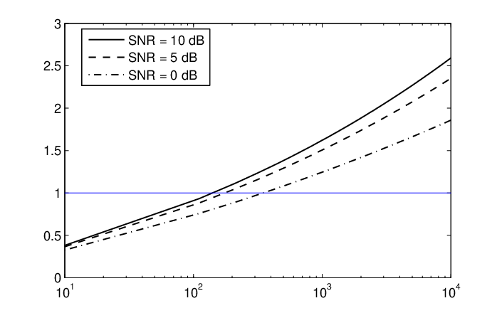
Figure 1: Normalizing factors βnk​(r)\beta^{k}_{n}(r) versus the number of users per super-cell KK, for M=3M=3, Q=2Q=2 Nt=2N_{t}=2 and γn,mk,r=1\gamma^{k,r}_{n,m}=1.
Number of users per super-cell K Normalizing factors ⁢ β k n ( r )

All the analyses are constructed on the basis that ∀k,n,r\forall k,n,r, we have βnk​(r)≥1\beta^{k}_{n}(r)\geq 1. As discussed earlier, under this condition, each user will have only one of its normalized 𝖲𝖨𝖭𝖱{\sf SINR}s (corresponding to different beamformers) greater than 1. Also, as implied throughout the analysis, at the asymptote of large KK, in each super-cell only Q​NtQN_{t} users will participate in the feedback processes, which is the core reason of having controlled amount of feedback. The condition βnk​(r)≥1\beta^{k}_{n}(r)\geq 1 can be guaranteed in the asymptote of large KK by recalling that Fnk​(βnk​(r),r)=1−1KF^{k}_{n}(\beta^{k}_{n}(r);r)=1-\frac{1}{K}. By numerically evaluating Fnk​(βnk​(r),r)F^{k}_{n}(\beta^{k}_{n}(r);r) through Monte Carlo realizations, Fig. 1 shows how the normalization factor changes with the number of users at 𝖲𝖭𝖱{\sf SNR}s. It is seen that in a network with M=3M=3 super-cells, each containing Q=2Q=2 cells and each base-station equipped with Nt=2N_{t}=2 transmit antennas the normalizing factors βnk​(r)\beta^{k}_{n}(r) very quickly exceed 1 (as the requirement of Lemma 1 on the conditional expected rates) for different 𝖲𝖭𝖱{\sf SNR} levels 0,50,5 and 10 dB. The normalization factors are obtained via numerically solving (3).

4.2 Throughput Scaling for Nr>1N_{r}>1

In this section we generalize the result of Theorem 1 (MISO capacity scaling) to MIMO networks with arbitrary number of receive antennas. As stated earlier in (7), by employing dirty-paper coding and facilitating full CSI feedback, the sum-rate throughput exhibits a double logarithmic growth with the number of receive antennas, NrN_{r}. We show that with slight modification to the scheduling procedure provided in Section 3 the same gain can be retained.

We modify the scheduling procedure such that it allows each user to receive more than one information stream across its different receive antennas. In other words, we preclude the receive antennas to jointly decode the information streams and consider different receive antennas as separate users. As a result, this translates to having effectively K​NrKN_{r} users in the network and all the analyses provided earlier for KK users can be extended for the network with K​NrKN_{r} users. It is noteworthy that although it might not be the most effective way to exploit the receive antennas, it yet achieves the optimal capacity scaling. Indeed, more sophisticated approaches involving joint signal decoding by the antenna arrays are expected to achieve the same gain. Based on this discussion, we modify the normalization factors βnk​(r)\beta^{k}_{n}(r) such that they satisfy

Fnk​(βnk​(r),r)=1−1K​Nr,F^{k}_{n}(\beta^{k}_{n}(r);r)=1-\frac{1}{KN_{r}}\ , (26)

and use the same normalization factor for all antennas of the same user. According to the modified scheduling algorithm on one hand, each user might be required to feed back the indices of more than one beam, which potentially increases the amount of feedback amount per user. On the other hand, increasing the normalization factor makes it more stringent for the users to satisfy their designated normalization factor constraints and send feedback. The discussions on the aggregate amount of feedback and effects of the number of users and number of receive antennas are given in Section 5. As a direct result of Theorem 1 (MISO capacity scaling) we obtain the following scaling law for MIMO networks.

Theorem 2 (MIMO Capacity Scaling)

For downlink transmission in a MIMO network with MM super-cells each with QQ base-stations, KK users per super-cell, NtN_{t} transmit antenna per base-station, and NrN_{r} receive antennas pre user, the sum-rate throughput achievable via the proposed scheduling procedure scales as

𝔼𝑯​[R]≐M​Q​Nt​log⁡log⁡K​Nr.\mathbb{E}_{{\boldsymbol{H}}}[R]\doteq MQN_{t}\log\log KN_{r}\ .

We remark that in the scheduling procedure we have considered that each user may receive more than one information stream. On the other hand, if we restrict each user to receive no more than one information stream, the performance will degrade. Indeed, as shown in [8] for single-cell broadcast transmissions, even with perfect 𝖲𝖨𝖭𝖱{\sf SINR} feedback, the sum-rate throughput scales as Nt​log⁡log​KN_{t}\log\log K which does not depend on the number of receive antennas. Therefore, with such restriction, adding more receiver antennas offers no asymptotic gain. Simulation results in Fig. 2 depict the sum-rate throughput achieved by the proposed scheduling scheme and show that it varies linearly with the number of super-cells MM and transmit antennas NtN_{t} and double logarithmically with the number of users KK.

Refer to caption
Figure 2: Sum-rate throughput versus the number of users per super-cell KK, for Q=2Q=2 and ρ=10\rho=10 dB. Each user has Nr=1N_{r}=1 receive antenna.
Number of users per super-cell K Sum-rate Throughput (bits/sec/Hz), = M 2 = N t 3 , = M 2 = N t 2 , = M 1 = N t 3 , = M 1 = N t 2

Finally, as a corollary to Theorem 2 we can recover the existing results on the capacity scaling of the single-cell broadcast channels. The result provided in the following corollary indicates that deploying the proposed scheduling scheme for only one super-cell, requires only finite-rate feedback and yet retains the optimal capacity scaling of the broadcast channels with full channel state information feedback. Similar to the results for the multi-cell networks, in the following corollary we also assume that the number of transmit and receive antennas Nt,NrN_{t},N_{r} are fixed.

Corollary 1 (Single-cell Capacity Scaling)

For a MIMO broadcast channel with NtN_{t} transmit antenna that serves KK users each equipped with NrN_{r} receive antennas, the sum-rate throughput achievable via the proposed scheduling procedure scales as

𝔼𝑯​[R]≐Nt​log⁡log⁡K​Nr.\mathbb{E}_{{\boldsymbol{H}}}[R]\doteq N_{t}\log\log KN_{r}\ .

5 Aggregate Feedback

So far we have established the sum-rate throughput scaling. In this section we evaluate the expected amount of feedback bits imposed by the proposed scheduling procedure. This essentially provides an upper bound on the minimum required amount of information exchange in the network. As discussed in Section 3, if a user meets the criterion to be considered as a candidate for being selected and scheduled, it will feed back ⌈log⁡Q​Nt⌉\lceil\log QN_{t}\rceil bits per eligible receive antenna, and otherwise will remain silent indicating that it is not a candidate for being scheduled. Therefore, each user, potentially, might send as many as min⁡(Nt,Nr)​⌈log⁡Q​Nt⌉\min(N_{t},N_{r})\lceil\log QN_{t}\rceil bits via the feedback channel. This, in turn, can potentially give rise to up to K​min⁡(Nt,Nr)​⌈log⁡Q​Nt⌉K\min(N_{t},N_{r})\lceil\log QN_{t}\rceil aggregate feedback bits in each super-cell, which can be prohibitive. Therefore, it is imperative to examine and control the burden put on the feedback channel.

Note that the normalization factors βnk​(r)\beta^{k}_{n}(r) change adaptively with varying KK. Therefore, as the number of users per super-cell increases, the chance that each individual user satisfies the normalization constraint becomes slimmer. In other words, the choices of βnk​(r)\beta^{k}_{n}(r) guarantee that as the network becomes dense, the aggregate feedback load is controlled via enforcing a more stringent constraint on each user to utilize the feedback channel. In practice, obtaining βnk​(r)\beta^{k}_{n}(r) through solving (3) can be carried out via bi-sectional search. As the CDF is an strictly increasing function in its argument and the problem in (3) has a unique solution, a simple bi-section search, which is computationally efficient, can solve the problem with arbitrary accuracy. In the next theorem we quantify the aggregate feedback and show that the expected aggregate feedback is a constant independent of the number of users in the network.

Theorem 3 (Aggregate Feedback)

For downlink transmission in a MIMO network with MM super-cells each with QQ base-stations, KK users per super-cell, NtN_{t} transmit antenna per base-station, and NrN_{r} receive antennas pre user, by deploying the proposed scheduling procedure, the aggregate feedback in the network is M​Q​Nt​⌈log⁡Q​Nt⌉MQN_{t}\lceil\log QN_{t}\rceil.

Proof: Lets define N=min⁡(Nt,Nr)N=\min(N_{t},N_{r}), which is the maximum number of information streams a user can receive. Also let 𝖲𝖨𝖭𝖱nk​(r,ℓ,i){\sf SINR}^{k}_{n}(r,\ell,i) denote the detection 𝖲𝖨𝖭𝖱{\sf SINR} of it​hi^{th} receive antenna of user UnkU^{k}_{n} when served along the beamforming vector 𝝎nr​(ℓ)\boldsymbol{\omega}^{r}_{n}(\ell). The probability that the it​hi^{th} receive antenna of user UnkU^{k}_{n} is a candidate to be served by one of the Q​NtQN_{t} beamformers of its designated super-cell, is upper bounded by

P⁡(maxr,ℓ⁡𝖲𝖨𝖭𝖱nk​(r,ℓ,i)βnk​(r)≥1)​≤union bound​∑r=1Q∑ℓ=1NtP⁡(𝖲𝖨𝖭𝖱nk​(r,ℓ,i)≥βnk​(r))=Q​NtK​Nr=△μ.P\Big(\max_{r,\;\ell}\frac{{\sf SINR}^{k}_{n}(r,\ell,i)}{\beta^{k}_{n}(r)}\geq 1\Big)\overset{\tiny\mbox{union bound}}{\leq}\sum_{r=1}^{Q}\sum_{\ell=1}^{N_{t}}P\Big({\sf SINR}^{k}_{n}(r,\ell,i)\geq\beta^{k}_{n}(r)\Big)=\frac{QN_{t}}{KN_{r}}\stackrel{{\scriptstyle\scriptscriptstyle\triangle}}{{=}}\mu\ .

Hence, the probability that exactly j≤Nj\leq N users satisfy the normalization constraint is upper bounded by μj=△(Nrj)​μj​(1−μ)Nr−j\mu_{j}\stackrel{{\scriptstyle\scriptscriptstyle\triangle}}{{=}}{N_{r}\choose j}\mu^{j}(1-\mu)^{N_{r}-j}. Therefore, by denoting the number of feedback bits per user by RnFBR_{n}^{\tiny{\rm FB}} and taking into account that if a user satisfies the normalization constraint, it will feed back ⌈log⁡Q​Nt⌉\lceil\log QN_{t}\rceil bits, we get

𝔼⁡[RFB]≤⌈log⁡Q​Nt⌉​∑j=1Nj​μj=⌈log⁡Q​Nt⌉​∑j=1Nj​(Nrj)​μj​(1−μ)Nr−j.\mathbb{E}[R^{\rm FB}]\leq\lceil\log QN_{t}\rceil\sum_{j=1}^{N}j\mu_{j}=\lceil\log QN_{t}\rceil\sum_{j=1}^{N}j{N_{r}\choose j}\mu^{j}(1-\mu)^{N_{r}-j}.

Hence, the aggregate amount of feedback in the nt​hn^{th} super-cell, denoted by 𝔼⁡[RnFB]\mathbb{E}[R^{\rm FB}_{n}] in the asymptote of large KK is

𝔼⁡[RnFB]\displaystyle\mathbb{E}[R^{\rm FB}_{n}] ≤\displaystyle\leq limK→∞K⁡⌈log⁡Q​Nt⌉​∑j=1Nj​(Nrj)​μj​(1−μ)Nr−j\displaystyle\lim_{K\rightarrow\infty}K\lceil\log QN_{t}\rceil\sum_{j=1}^{N}j{N_{r}\choose j}\mu^{j}(1-\mu)^{N_{r}-j} (27)
=\displaystyle= ⌈log⁡Q​Nt⌉​∑j=1Nj​(Nrj)​limK→∞(Q​NtK​Nr)j​(1−Q​NtK​Nr)Nr−j1K\displaystyle\lceil\log QN_{t}\rceil\sum_{j=1}^{N}j{N_{r}\choose j}\lim_{K\rightarrow\infty}\frac{\Big(\frac{QN_{t}}{KN_{r}}\Big)^{j}\Big(1-\frac{QN_{t}}{KN_{r}}\Big)^{N_{r}-j}}{\frac{1}{K}}
=\displaystyle= ⌈log⁡Q​Nt⌉​∑j=1Nj​(Nrj)​(Q​NtNr)j​limK→∞1Kj−1\displaystyle\lceil\log QN_{t}\rceil\sum_{j=1}^{N}j{N_{r}\choose j}\Big(\frac{QN_{t}}{N_{r}}\Big)^{j}\lim_{K\rightarrow\infty}\frac{1}{K^{j-1}}
=\displaystyle= Q​Nt​⌈log⁡Q​Nt⌉,\displaystyle QN_{t}\lceil\log QN_{t}\rceil\ ,

which provides that the expected aggregate amount of feedback bits in the network does not exceed M​Q​Nt​⌈log⁡Q​Nt⌉MQN_{t}\lceil\log QN_{t}\rceil. The last equality holds by noting that for j>1j>1 the term 1Kj−1→0\frac{1}{K^{j-1}}\rightarrow 0 and the only non-zero term corresponds to j=1j=1 and is equal to Q​Nt​⌈log⁡Q​Nt⌉QN_{t}\lceil\log QN_{t}\rceil.   

The simulation results provided in Fig. 3 quantify the aggregate amount of feedback imposed by our scheduling protocol to the feedback channel. As anticipated by the analyses, as the number of users increase, the total amount of feedback bits is Q​Nt​⌈log⁡Q​Nt⌉QN_{t}\lceil\log QN_{t}\rceil which is independent of the number of users as well as the number of receive antennas. This implies that as the number of users increase, only Q​NtQN_{t} users will participate in feeding back their indices of their desired beams. This is due to the fact that high normalizing factors for networks with large number of users, only allow the best Q​NtQN_{t} users to feed back the indices of their corresponding beams. For the simulations we consider the settings Q=1,2Q=1,2 base-stations per super-cell and assume that each user has Nr=3N_{r}=3 receive antennas.

Refer to caption
Figure 3: Aggregate amount of feedback versus the number of users per super-cell KK. Each user has Nr=1N_{r}=1 receive antennas and ρ=10\rho=10 dB.
Number of users per super-cell K Sum-rate Feedback E [ R FB n ] , = Q 2 = N t 4 ⁢ 16 log 2 8 , = Q 2 = N t 3 ⁢ 12 log 2 6 , = Q 2 = N t 2 ⁢ 8 log 2 4 , = Q 1 = N t 3 ⁢ 6 log 2 3 , = Q 1 = N t 2 ⁢ 4 log 2 2

6 Practical Issues

6.1 Size of Super-cells

The size of the super-cells QQ impacts both the scaling rate of the sum-rate throughput (Theorem 1 on the MISO capacity scaling) as well as the amount of information exchange in the network (Theorem 3 on aggregate feedback). The capacity scaling analysis shows that the sum-rate throughput scales as M​Q​Nt​log⁡log⁡K​NrMQN_{t}\log\log KN_{r}. This is the scaling of a network with a total number of M​QMQ base-stations and M​KMK users, which means there exist T=△KQT\stackrel{{\scriptstyle\scriptscriptstyle\triangle}}{{=}}\frac{K}{Q} users per base-station. When keeping this ratio of users per base-station constant, the sum-rate throughput scales as M​Q​Nt​log⁡log⁡Q​T​NrMQN_{t}\log\log QTN_{r}. This scaling essentially implies that as long as the product M​QMQ is a constant, the sum-rate scaling remains unchanged. The reason is that for fixed M​QMQ, necessarily MM will be a finite integer, based on which we have

limK→∞𝔼𝑯​[R]M​Q​Nt​log⁡log⁡M​K​Nr=limK→∞log⁡log​K​Nrlog⁡log​M​K​Nr=1,\lim_{K\rightarrow\infty}\frac{\mathbb{E}_{{\boldsymbol{H}}}[R]}{MQN_{t}\log\log MKN_{r}}=\lim_{K\rightarrow\infty}\frac{\log\log KN_{r}}{\log\log MKN_{r}}=1,

which implies that the throughput of the proposed procedure scales identical to the scaling law provided in Theorem 2. Therefore, when the total number of base-stations in the network M​QMQ is fixed, irrespectively of how we cluster them to construct the super-cells, the scaling law remains fixed. On the other hand, from Theorem 1 (MISO capacity scaling), the aggregate amount of information exchange is upper bounded by M​Q​Nt​⌈log⁡Q​Nt⌉MQN_{t}\lceil\log QN_{t}\rceil. Once having a fixed number of base-stations in the network, i.e., M​QMQ is fixed, the amount of information exchange is clearly minimized by setting Q=1Q=1. This choice of QQ corresponds to the setting that there is no cooperation among the base-stations and each base-station acts independently of others. This fact in conjunction with the freedom in clustering the network shows that even when the network is completely distributed (no base-station cooperation) by exchanging as low as M​Nt​log⁡NtMN_{t}\log N_{t} information bits, still the optimal sum-rate throughput scaling is achievable.

There exists, however, a cost associated with such distributed downlink transmission. While the sum-rate throughput of the proposes scheme and that of dirty-paper coding scale identically, there exists a gap between them. The distributed processing penalizes the performance by enlarging this gap. By increasing the size of the super-cells QQ we can reduce this gap, which shows that we can trade additional information exchange in favor of increasing the achievable sum-rate throughput, which is expected intuitively. The monte-carlo simulation results in Fig. 4 depicts the impact of clustering on the achievable sum-rate throughput. We consider a network containing M​Q=6MQ=6 base-stations and look into the sum-rate of the four possible clustering cases of (M,Q)=(6,1),(3,2),(2,3)(M,Q)=(6,1),(3,2),(2,3) and (1,6). While all four cases exhibit identical scalings, it is observed allowing more level of cooperation among the base-stations, i.e., large clusters sizes QQ, improves the sum-rate throughput. For the simulations we have considered the two cases of Nt=1,4N_{t}=1,4 and have assumed that the users have Nr=3N_{r}=3 receive antennas and ρ=10\rho=10 dB.

Refer to caption
Figure 4: The impact of super-cell sizes QQ on the achievable sum-rate throughput.
Total number of users in the network ⁢ M K Sum-rate Throughput (bits/sec/Hz) = N t 2 = N t 4

6.2 Fairness

In a non-homogenous network the reception quality at various users not only is influenced by how their channel direction vectors are aligned with the beam direction, but also is impacted by the path-loss and the shadowing they experience. As scheduling in our scheme involves opportunistic selection of the users who have satisfied a minimum level of reception quality, the system might be dominated by the user with the strongest reception qualities. In general, there exist an inherent tension between opportunistic user selection and maintaining some notion of fairness among the users. Therefore, it is imperative to investigate how such opportunistic user selection affects fairness.

It is, interestingly, observed that by deploying the proposed scheduling procedure, fairness, in the sense that all users are equiprobable to be served by the base-stations, is maintained. Such fairness is preserved as we assign different normalization factors to the users with different path-loss and shadowing (γm,nk,r\gamma^{k,r}_{m,n}). This argument is formalized in the next theorem.

Theorem 4 (Fairness)

For downlink transmission in a MIMO network with MM super-cells each with QQ base-stations, KK users per super-cell, NtN_{t} transmit antenna per base-station, and NrN_{r} receive antennas pre user, all users are equally likely to be served by the proposed scheduling procedure.

Proof: The proof relies on the choices of the normalization factors given in (26). Let us define 𝖲𝖨𝖭𝖱nk​(r,ℓ,i){\sf SINR}^{k}_{n}(r,\ell,i) as received 𝖲𝖨𝖭𝖱{\sf SINR} of the it​hi^{th} receive antenna of user UnkU^{k}_{n} when served along the beamforming vector 𝝎nr​(ℓ)\boldsymbol{\omega}^{r}_{n}(\ell). By following the same line of argument as in (25) and taking into account (26), the probability that the it​hi^{th} receive antenna of user UnkU^{k}_{n} is a candidate to be scheduled with the beamformer 𝝎nr​(ℓ)\boldsymbol{\omega}^{r}_{n}(\ell) is

θn=△P⁡(𝖲𝖨𝖭𝖱nk​(r,ℓ,i)≥βnk​(r))=1−Fnk​(βnk​(r),r)=1K​Nr,\theta_{n}\stackrel{{\scriptstyle\scriptscriptstyle\triangle}}{{=}}P\Big({\sf SINR}^{k}_{n}(r,\ell,i)\geq\beta^{k}_{n}(r)\Big)=1-F^{k}_{n}(\beta^{k}_{n}(r);r)=\frac{1}{KN_{r}}\ , (28)

which is identical for all users (in the nt​hn^{th} super-cell) and all transmit and receive antennas. Therefore, the probability that exactly j≤min⁡(Nt,Nr)j\leq\min(N_{t},N_{r}) number of the receive antennas of user kk being eligible to be served by a base-station is

θnj=△(Ntj)​θnj​(1−θn)Nt−j,\theta^{j}_{n}\stackrel{{\scriptstyle\scriptscriptstyle\triangle}}{{=}}{N_{t}\choose j}\theta_{n}^{j}(1-\theta_{n})^{N_{t}-j},

which is also identical for all users in the nt​hn^{th} super-cell. Therefore, all users in each super-cell are equally likely to be scheduled for receiving any certain number of information streams.   

6.3 Training

As briefly mentioned at the end of Section 3 each user needs to calculate the 𝖲𝖨𝖭𝖱{\sf SINR}s that each of the beamformers can sustain for carrying the information intended for that user. Acquiring such 𝖲𝖨𝖭𝖱{\sf SINR}s is viable during the training interval. Such training being carried out on the downlink channel will cost downlink bandwidth. Nevertheless, it can be readily shown that such bandwidth loss does not penalize the throughput scaling rate. More specifically, due to the broadcast nature of the wireless channels, the base-stations will transmit a common training message for all users. The duration of such training will be fixed and independent of the number of users in the network. If we denote the fixed throughput loss due to such training by R𝗍𝗋𝖺𝗂𝗇R_{\sf train}, then the throughput after penalizing it by the training bandwidth loss will be 𝔼𝑯​[R]−R𝗍𝗋𝖺𝗂𝗇\mathbb{E}_{{\boldsymbol{H}}}[R]-R_{\sf train}. R𝗍𝗋𝖺𝗂𝗇R_{\sf train} being fixed provides that for increasing KK, 𝔼𝑯​[R]−R𝗍𝗋𝖺𝗂𝗇\mathbb{E}_{{\boldsymbol{H}}}[R]-R_{\sf train} will scale similar to 𝔼𝑯​[R]\mathbb{E}_{{\boldsymbol{H}}}[R]. Therefore, while training incurs a loss on the throughput, it will not affect the throughput scaling rate provided in Theorem 2.

7 Conclusions

In this paper we have assessed the minimum amount of information exchange required in a multi-cell multiuser downlink transmission with base-station cooperation, in order to retain the optimal capacity scaling. By providing a constructive proof we have demonstrated that by an appropriate design of a feedback mechanism for each super-cell, we can avoid any cross-(super) cellular information exchange and yet achieve the optimal scaling law. More specifically, for a MIMO network consisting of MM super-cells, each consisting of QQ base-stations that carry out the downlink transmission collaboratively, when each base-station is equipped with NtN_{t} transmit antennas, exchanging M​Q​Nt​⌈log⁡Q​Nt⌉MQN_{t}\lceil\log QN_{t}\rceil information bits across the network suffices to guarantee the achievability of the optimal scaling of the sum-rate throughput. This result relies on a constructive proof, where we offer a scheduling framework that satisfies the information exchange constraints. Furthermore, the scheme also provides good performance for practical networks and sustain fairness among the users in the network.

Appendix A Proof of Lemma 1 (Conditional Expected Rates)

Scheme of the Proof:

ℋnr​(ℓ)={k|𝗌𝗂𝗇𝗋nk​(r,ℓ)≥1}.{\cal H}^{r}_{n}(\ell)=\{k\;|\;{\sf sinr}^{k}_{n}(r,\ell)\geq 1\}\ . (29)

This is due to the fact that when βnk​(r)≥1\beta^{k}_{n}(r)\geq 1, each user in the super-cell 𝒬n{\cal Q}_{n} will have a normalized 𝖲𝖨𝖭𝖱{\sf SINR} greater than 1 for at most one of Q​NtQN_{t} beamformers {𝝎nr​(ℓ)}r,ℓ\{\boldsymbol{\omega}^{r}_{n}(\ell)\}_{r,\ell}, i.e., if a user has a normalized 𝖲𝖨𝖭𝖱≥1{\sf SINR}\geq 1 for a beamformer, its normalized 𝖲𝖨𝖭𝖱{\sf SINR} for the rest of beamformers is smaller than 1. This can be readily verified by noting that when βnk​(r)≥1\beta^{k}_{n}(r)\geq 1 the we have

𝗌𝗂𝗇𝗋nk​(r,ℓ)≥1\displaystyle{\sf sinr}^{k}_{n}(r,\ell)\geq 1\quad ⇒(4)𝖲𝖨𝖭𝖱nk​(r,ℓ)≥βnk​(r)≥1⇒(2)𝖲𝖨𝖭𝖱nk​(r′,ℓ′)<1∀(r′,ℓ′)≠(r,ℓ)\displaystyle\overset{\eqref{eq:sinrn}}{\Rightarrow}\quad{\sf SINR}^{k}_{n}(r,\ell)\geq\beta^{k}_{n}(r)\geq 1\quad\overset{\eqref{eq:sinr}}{\Rightarrow}\quad{\sf SINR}^{k}_{n}(r^{\prime},\ell^{\prime})<1\quad\forall(r^{\prime},\ell^{\prime})\neq(r,\ell)
⇒(4)𝗌𝗂𝗇𝗋nk​(r′,ℓ′)<1∀(r′,ℓ′)≠(r,ℓ)\displaystyle\overset{\eqref{eq:sinrn}}{\Rightarrow}\quad{\sf sinr}^{k}_{n}(r^{\prime},\ell^{\prime})<1\quad\forall(r^{\prime},\ell^{\prime})\neq(r,\ell)

Given the above characterization of ℋnr​(ℓ){\cal H}^{r}_{n}(\ell) in (29), the rest of the proof has three major steps. In the first step by using the characterization of ℋnr​(ℓ){\cal H}^{r}_{n}(\ell) and some simple manipulation the conditional expected value of the rate 𝔼𝑯​[Rnr​(ℓ)|ℋnr​(ℓ)]\mathbb{E}_{\boldsymbol{H}}[R^{r}_{n}(\ell)\;|\;{\cal H}^{r}_{n}(\ell)] is reformulated. In the second step, we find a lower bound on this conditional expected rate. This lower bound itself is also a conditional expected rate with a different condition compared with 𝔼𝑯​[Rnr​(ℓ)|ℋnr​(ℓ)]\mathbb{E}_{\boldsymbol{H}}[R^{r}_{n}(\ell)\;|\;{\cal H}^{r}_{n}(\ell)]. Finally, in the third step we show how removing these new conditions from the conditional expected rates will provide a new lower bound on 𝔼𝑯​[Rnr​(ℓ)|ℋnr​(ℓ)]\mathbb{E}_{\boldsymbol{H}}[R^{r}_{n}(\ell)\;|\;{\cal H}^{r}_{n}(\ell)] which is appropriate related to the order statistics of the set {𝖲𝖨𝖭𝖱n1​(r,ℓ),…,𝖲𝖨𝖭𝖱nK​(r,ℓ)}\{{\sf SINR}^{1}_{n}(r,\ell),\dots,{\sf SINR}^{K}_{n}(r,\ell)\}.

Step 1) Reformulating 𝔼H​[Rnr​(ℓ)|ℋnr​(ℓ)]\mathbb{E}_{\boldsymbol{H}}[R^{r}_{n}(\ell)\;|\;{\cal H}^{r}_{n}(\ell)]:
By recalling (9) we have

𝔼𝑯​[Rnr​(ℓ)|ℋnr​(ℓ)]=1|ℋnr​(ℓ)|​∑k∈ℋnr​(ℓ)𝔼𝑯​[log⁡(1+𝖲𝖨𝖭𝖱nk​(r,ℓ))|ℋnr​(ℓ)].\displaystyle\mathbb{E}_{\boldsymbol{H}}[R^{r}_{n}(\ell)\;|\;{\cal H}^{r}_{n}(\ell)]=\frac{1}{|{\cal H}^{r}_{n}(\ell)|}\sum_{k\in{\cal H}^{r}_{n}(\ell)}\mathbb{E}_{\boldsymbol{H}}\left[\log\left(1+{\sf SINR}^{k}_{n}(r,\ell)\right)\;\big|\;{\cal H}^{r}_{n}(\ell)\right]. (30)

On the other hand, from (29) we have

∀k∈ℋnr​(ℓ):𝗌𝗂𝗇𝗋nk​(r,ℓ)≥1and∀k′∉ℋnr​(ℓ):𝗌𝗂𝗇𝗋nk′​(ℓ)<1.\forall k\in{\cal H}^{r}_{n}(\ell):{\sf sinr}^{k}_{n}(r,\ell)\geq 1\hskip 14.45377pt\mbox{and}\hskip 14.45377pt\forall k^{\prime}\notin{\cal H}^{r}_{n}(\ell):{\sf sinr}^{k^{\prime}}_{n}(\ell)<1\ . (31)

By combining (30) and (31) we find that

𝔼𝑯​[Rnr​(ℓ)|ℋnr​(ℓ)]\displaystyle\hskip 0.0pt\mathbb{E}_{\boldsymbol{H}}[R^{r}_{n}(\ell)\;|\;{\cal H}^{r}_{n}(\ell)]
=1|ℋnr​(ℓ)|∑k∈ℋnr​(ℓ)𝔼𝑯[log(1+𝖲𝖨𝖭𝖱nk(r,ℓ))|∀k∈ℋnr(ℓ):𝗌𝗂𝗇𝗋nk(r,ℓ)≥1;\displaystyle=\frac{1}{|{\cal H}^{r}_{n}(\ell)|}\sum_{k\in{\cal H}^{r}_{n}(\ell)}\mathbb{E}_{{\boldsymbol{H}}}\bigg[\log\Big(1+{\sf SINR}^{k}_{n}(r,\ell)\Big)\;\big|\;\forall k\in{\cal H}^{r}_{n}(\ell):{\sf sinr}^{k}_{n}(r,\ell)\geq 1;
and∀k′∉ℋnr(ℓ):𝗌𝗂𝗇𝗋nk′(ℓ)<1]\displaystyle\hskip 238.49121pt\mbox{and}\quad\forall k^{\prime}\notin{\cal H}^{r}_{n}(\ell):{\sf sinr}^{k^{\prime}}_{n}(\ell)<1\;\bigg]
=1|ℋnr​(ℓ)|∑k∈ℋnr​(ℓ)𝔼𝑯[log(1+𝖲𝖨𝖭𝖱nk(r,ℓ))|∀k∈ℋnr(ℓ):𝖲𝖨𝖭𝖱nk(r,ℓ)≥βnk(r);\displaystyle=\frac{1}{|{\cal H}^{r}_{n}(\ell)|}\sum_{k\in{\cal H}^{r}_{n}(\ell)}\mathbb{E}_{{\boldsymbol{H}}}\bigg[\log\Big(1+{\sf SINR}^{k}_{n}(r,\ell)\Big)\;\big|\;\forall k\in{\cal H}^{r}_{n}(\ell):{\sf SINR}^{k}_{n}(r,\ell)\geq\beta^{k}_{n}(r);
and∀k′∉ℋnr(ℓ):𝖲𝖨𝖭𝖱nk′(ℓ)<βnk′(r)],\displaystyle\hskip 238.49121pt\mbox{and}\quad\forall k^{\prime}\notin{\cal H}^{r}_{n}(\ell):{\sf SINR}^{k^{\prime}}_{n}(\ell)<\beta^{k^{\prime}}_{n}(r)\bigg]\ , (32)

where in the first equality we have replaced (31) into (30) and in the second equality we have invoked that 𝗌𝗂𝗇𝗋nk​(r,ℓ)=𝖲𝖨𝖭𝖱nk​(r,ℓ)βnk​(r){\sf sinr}^{k}_{n}(r,\ell)=\frac{{\sf SINR}^{k}_{n}(r,\ell)}{\beta^{k}_{n}(r)}.

Step 2) Lower Bound on 𝔼H​[Rnr​(ℓ)|ℋnr​(ℓ)]\mathbb{E}_{\boldsymbol{H}}[R^{r}_{n}(\ell)\;|\;{\cal H}^{r}_{n}(\ell)]:
In the next step we manipulate the conditions of the expected rate given in (32) and obtain a more tractable lower bound on 𝔼𝑯​[Rnr​(ℓ)|ℋnr​(ℓ)]\mathbb{E}_{\boldsymbol{H}}[R^{r}_{n}(\ell)\;|\;{\cal H}^{r}_{n}(\ell)]. The core of such manipulation is given in the following lemma.

Lemma 6 (Conditional Expectation)

For a random variable XX, increasing function g⁡(⋅)g(\cdot) and real values b≥ab\geq a that belong to the support of XX we have

𝔼⁡[g⁡(X)|X≥b]≥𝔼⁡[g⁡(X)|X≥a].\mathbb{E}\Big[g(X)\;|\;X\geq b\Big]\geq\mathbb{E}\Big[g(X)\;|\;X\geq a\Big]. (33)

Proof: Define Y=△g⁡(X)Y\stackrel{{\scriptstyle\scriptscriptstyle\triangle}}{{=}}g(X) and denote the CDFs of XX and YY by FX​(x)F_{X}(x) and Fy​(y)F_{y}(y), respectively.

𝔼⁡[g⁡(X)|X≥b]\displaystyle\mathbb{E}\Big[g(X)\;|\;X\geq b\Big] =∫yy​d​(FY|X≥b​(y))=∫01FY|X≥b−1​(u)​𝑑u.\displaystyle=\int_{y}y\;d\big(F_{Y\;|\;X\geq b}(y)\big)=\int_{0}^{1}\;F^{-1}_{Y\;|\;X\geq b}(u)\;du\ . (34)

On the other hand, by recalling that g⁡(X)g(X) is monotonic in XX

FY|X≥b​(y)\displaystyle F_{Y\;|\;X\geq b}(y) =P⁡(g⁡(X)≤y|X≥b)=P⁡(b≤X≤g−1​(y))P⁡(b≤X)=FX​(g−1​(y))−FX​(b)1−FX​(b)\displaystyle=P(g(X)\leq y\;|\;X\geq b)=\frac{P(b\leq X\leq g^{-1}(y))}{P(b\leq X)}=\frac{F_{X}(g^{-1}(y))-F_{X}(b)}{1-F_{X}(b)}
≤FX​(g−1​(y))−FX​(a)1−FX​(a)=P⁡(g⁡(X)≤y|X≥a)\displaystyle\leq\frac{F_{X}(g^{-1}(y))-F_{X}(a)}{1-F_{X}(a)}=P(g(X)\leq y\;|\;X\geq a)
=FY|X≥a​(y),\displaystyle=F_{Y\;|\;X\geq a}(y)\ ,

which yields that

∀u∈[0,1]:FY|X≥b−1​(u)≥FY|X≥a−1​(u).\forall u\in[0,1]:\quad F^{-1}_{Y\;|\;X\geq b}(u)\geq F^{-1}_{Y\;|\;X\geq a}(u)\ . (35)

Equations (34) and (35) provide that

𝔼⁡[g⁡(X)|X≥b]≥∫01FY|X≥a−1​(u)​𝑑u=∫yy​d​(FY|X≥a​(y))=𝔼⁡[g⁡(X)|X≥a].\mathbb{E}\Big[g(X)\;|\;X\geq b\Big]\geq\int_{0}^{1}\;F^{-1}_{Y\;|\;X\geq a}(u)\;du=\int_{y}y\;d\big(F_{Y\;|\;X\geq a}(y)\big)=\mathbb{E}\Big[g(X)\;|\;X\geq a\Big]\ .


Next we construct a hypothetical event under which the users in ℋnr​(ℓ){\cal H}^{r}_{n}(\ell) satisfy some other 𝖲𝖨𝖭𝖱{\sf SINR} constraints. For this purpose, we introduce the set of users ℋ~nr​(ℓ)\tilde{\cal H}^{r}_{n}(\ell) corresponding to ℋnr​(ℓ){\cal H}^{r}_{n}(\ell) such that

ℋ~nr​(ℓ)=△{k|𝖲𝖨𝖭𝖱nk​(r,ℓ)≥mini⁡βni​(r)}.\tilde{\cal H}^{r}_{n}(\ell)\stackrel{{\scriptstyle\scriptscriptstyle\triangle}}{{=}}\{k\;|\;{\sf SINR}^{k}_{n}(r,\ell)\geq\min_{i}\beta^{i}_{n}(r)\}\ . (36)

Now consider a hypothetical channel condition for which the event ℋ~nr​(ℓ)\tilde{\cal H}^{r}_{n}(\ell) includes the same set of users as the the event ℋnr​(ℓ){\cal H}^{r}_{n}(\ell) does. Under this hypothetical conditions, i.e., ℋ~nr​(ℓ)=ℋnr​(ℓ)\tilde{\cal H}^{r}_{n}(\ell)={\cal H}^{r}_{n}(\ell), by recalling the characterization of 𝔼𝑯​[Rnr​(ℓ)|ℋnr​(ℓ)]\mathbb{E}_{\boldsymbol{H}}[R^{r}_{n}(\ell)\;|\;{\cal H}^{r}_{n}(\ell)] given in (32) we set b=βnk​(r)b=\beta^{k}_{n}(r) and a=mini⁡βni​(r)a=\min_{i}\beta^{i}_{n}(r) and replace the conditions 𝖲𝖨𝖭𝖱nk​(r,ℓ)≥βnk​(r){\sf SINR}^{k}_{n}(r,\ell)\geq\beta^{k}_{n}(r) by 𝖲𝖨𝖭𝖱nk​(r,ℓ)≥mini⁡βni​(r){\sf SINR}^{k}_{n}(r,\ell)\geq\min_{i}\beta^{i}_{n}(r). By noting that b≥ab\geq a from Lemma 6 we obtain

𝔼𝑯​[Rnr​(ℓ)|ℋnr​(ℓ)]\displaystyle\mathbb{E}_{\boldsymbol{H}}[R^{r}_{n}(\ell)\;|\;{\cal H}^{r}_{n}(\ell)]
≥(33)1|ℋnr​(ℓ)|∑k∈ℋ~nr​(ℓ)𝔼𝑯[log(1+𝖲𝖨𝖭𝖱nk(r,ℓ))|∀k∈ℋ~nr(ℓ):𝖲𝖨𝖭𝖱nk(r,ℓ)≥miniβni(r);\displaystyle\overset{\eqref{eq:lemma:condition}}{\geq}\frac{1}{|{\cal H}^{r}_{n}(\ell)|}\sum_{k\in\tilde{\cal H}^{r}_{n}(\ell)}\mathbb{E}_{{\boldsymbol{H}}}\bigg[\log\Big(1+{\sf SINR}^{k}_{n}(r,\ell)\Big)\;\big|\;\forall k\in\tilde{\cal H}^{r}_{n}(\ell):{\sf SINR}^{k}_{n}(r,\ell)\geq\min_{i}\beta^{i}_{n}(r);
and∀k′∉ℋ~nr(ℓ):𝖲𝖨𝖭𝖱nk′(ℓ)<βnk′(r)].\displaystyle\hskip 198.7425pt\mbox{and}\quad\forall k^{\prime}\notin\tilde{\cal H}^{r}_{n}(\ell):{\sf SINR}^{k^{\prime}}_{n}(\ell)<\beta^{k^{\prime}}_{n}(r)\bigg]\ . (37)

Next, by taking into account the statistical independence of 𝖲𝖨𝖭𝖱nk​(r,ℓ){\sf SINR}^{k}_{n}(r;\ell) and 𝖲𝖨𝖭𝖱nk′​(r,ℓ){\sf SINR}^{k^{\prime}}_{n}(r;\ell) for k∈ℋ~nr​(ℓ)k\in\tilde{\cal H}^{r}_{n}(\ell) and k′∉ℋ~nr​(ℓ)k^{\prime}\notin\tilde{\cal H}^{r}_{n}(\ell), which is due to the statistical independence of channel matrices 𝑯n,mk,r{\boldsymbol{H}}^{k,r}_{n,m} and 𝑯n,mk′,r{\boldsymbol{H}}^{k^{\prime},r}_{n,m}, changing the conditions enforced on 𝖲𝖨𝖭𝖱nk′​(r,ℓ){\sf SINR}^{k^{\prime}}_{n}(r;\ell) for k′∉ℋ~nr​(ℓ)k^{\prime}\notin\tilde{\cal H}^{r}_{n}(\ell) does not affect the statistics of 𝖲𝖨𝖭𝖱nk​(ℓ){\sf SINR}^{k}_{n}(\ell) for k∈ℋ~nr​(ℓ)k\in\tilde{\cal H}^{r}_{n}(\ell). Therefore, slightly changing the conditions 𝖲𝖨𝖭𝖱nk′​(ℓ)<βnk′​(r){\sf SINR}^{k^{\prime}}_{n}(\ell)<\beta^{k^{\prime}}_{n}(r) to 𝖲𝖨𝖭𝖱nk′​(ℓ)<mini⁡βni​(r){\sf SINR}^{k^{\prime}}_{n}(\ell)<\min_{i}\beta^{i}_{n}(r) for all k′∉ℋ~nr​(ℓ)k^{\prime}\notin\tilde{\cal H}^{r}_{n}(\ell) does not change the distribution of 𝖲𝖨𝖭𝖱nk​(r,ℓ){\sf SINR}^{k}_{n}(r,\ell) and (37) can be equivalently cast as

𝔼𝑯​[Rnr​(ℓ)|ℋnr​(ℓ)]\displaystyle\mathbb{E}_{\boldsymbol{H}}[R^{r}_{n}(\ell)\;|\;{\cal H}^{r}_{n}(\ell)]
≥1|ℋnr​(ℓ)|∑k∈ℋ~nr​(ℓ)𝔼𝑯[log(1+𝖲𝖨𝖭𝖱nk(r,ℓ))|∀k∈ℋ~nr(ℓ):𝖲𝖨𝖭𝖱nk(r,ℓ)≥miniβni(r);\displaystyle\geq\frac{1}{|{\cal H}^{r}_{n}(\ell)|}\sum_{k\in\tilde{\cal H}^{r}_{n}(\ell)}\mathbb{E}_{{\boldsymbol{H}}}\bigg[\log\Big(1+{\sf SINR}^{k}_{n}(r,\ell)\Big)\;\big|\;\forall k\in\tilde{\cal H}^{r}_{n}(\ell):{\sf SINR}^{k}_{n}(r,\ell)\geq\min_{i}\beta^{i}_{n}(r);
and∀k′∉ℋ~nr(ℓ):𝖲𝖨𝖭𝖱nk′(ℓ)<miniβni(r)].\displaystyle\hskip 191.51505pt\mbox{and}\quad\forall k^{\prime}\notin\tilde{\cal H}^{r}_{n}(\ell):{\sf SINR}^{k^{\prime}}_{n}(\ell)<\min_{i}\beta^{i}_{n}(r)\bigg]\ . (38)

The new condition

∀k∈ℋ~nr​(ℓ):𝖲𝖨𝖭𝖱nk​(r,ℓ)≥mini⁡βni​(r)and∀k′∉ℋ~nr​(ℓ):𝖲𝖨𝖭𝖱nk′​(ℓ)<mini⁡βni​(r),\forall k\in\tilde{\cal H}^{r}_{n}(\ell):{\sf SINR}^{k}_{n}(r,\ell)\geq\min_{i}\beta^{i}_{n}(r)\quad\mbox{and}\quad\forall k^{\prime}\notin\tilde{\cal H}^{r}_{n}(\ell):{\sf SINR}^{k^{\prime}}_{n}(\ell)<\min_{i}\beta^{i}_{n}(r)\ ,

implies that under this condition, the set ℋ~nr​(ℓ)\tilde{\cal H}^{r}_{n}(\ell) contains the |ℋ~nr​(ℓ)|=|ℋnr​(ℓ)||\tilde{\cal H}^{r}_{n}(\ell)|=|{\cal H}^{r}_{n}(\ell)| largest values of the set

{𝖲𝖨𝖭𝖱n1​(r,ℓ),…,𝖲𝖨𝖭𝖱nK​(r,ℓ)},\{{\sf SINR}^{1}_{n}(r,\ell),\dots,{\sf SINR}^{K}_{n}(r,\ell)\}\ ,

and the lower bound on 𝔼𝑯​[Rnr​(ℓ)|ℋnr​(ℓ)]\mathbb{E}_{\boldsymbol{H}}[R^{r}_{n}(\ell)\;|\;{\cal H}^{r}_{n}(\ell)] given in (38) is the arithmetic average of these |ℋnr​(ℓ)||{\cal H}^{r}_{n}(\ell)| largest values conditioned on the constraint that they are larger than or equal to mini⁡βni​(r)\min_{i}\beta^{i}_{n}(r) and the remaining (K−|ℋnr​(ℓ)|)(K-|{\cal H}^{r}_{n}(\ell)|) 𝖲𝖨𝖭𝖱{\sf SINR} values are smaller than mini⁡βni​(r)\min_{i}\beta^{i}_{n}(r). This interpretation can be formalized as follows.

𝔼𝑯​[Rnr​(ℓ)|ℋnr​(ℓ)]\displaystyle\mathbb{E}_{\boldsymbol{H}}[R^{r}_{n}(\ell)\;|\;{\cal H}^{r}_{n}(\ell)]
≥1|ℋnr​(ℓ)|​∑j=1|ℋnr​(ℓ)|𝔼𝑯​[log⁡(1+𝖲𝖨𝖭𝖱n(j)​(r,ℓ))|𝖲𝖨𝖭𝖱n(A)​(r,ℓ)≥mini⁡βni​(r)>𝖲𝖨𝖭𝖱n(A+1)​(r,ℓ)],\displaystyle\geq\frac{1}{|{\cal H}^{r}_{n}(\ell)|}\sum_{j=1}^{|{\cal H}^{r}_{n}(\ell)|}\mathbb{E}_{{\boldsymbol{H}}}\bigg[\log\Big(1+{\sf SINR}_{n}^{(j)}(r,\ell)\Big)\;\big|\;{\sf SINR}_{n}^{(A)}(r,\ell)\geq\min_{i}\beta^{i}_{n}(r)>{\sf SINR}_{n}^{(A+1)}(r,\ell)\bigg]\ , (39)

where we have defined A=△|ℋnr​(ℓ)|A\stackrel{{\scriptstyle\scriptscriptstyle\triangle}}{{=}}|{\cal H}^{r}_{n}(\ell)|.

Step 3) Removing the Condition in (39):
In the final step, we further simplify the lower bound on 𝔼𝑯​[Rnr​(ℓ)|ℋnr​(ℓ)]\mathbb{E}_{\boldsymbol{H}}[R^{r}_{n}(\ell)\;|\;{\cal H}^{r}_{n}(\ell)] provided in (39). This step will be the immediate application of the following lemma.

Lemma 7 (Conditional Expected Value of the Order Statistics)

Consider the set of independent random variables {X1,…,XK}\{X_{1},\dots,X_{K}\} and its corresponding set of order statistics {X(1),…,X(K)}\{X^{(1)},\dots,X^{(K)}\}. For any increasing function g⁡(⋅)g(\cdot) and the real value aa belonging to the supports of XkX_{k} we have

∀j≤l:𝔼⁡[g⁡(X(j))|X(l+1)≤a≤X(l)]≥𝔼⁡[g⁡(X(j))].\forall\;j\leq l:\quad\mathbb{E}\left[g\big(X^{(j)}\big)\;\big|\;X^{(l+1)}\leq a\leq X^{(l)}\right]\geq\mathbb{E}\left[g\big(X^{(j)}\big)\right]\ . (40)

Proof: In the first step, by following the same line of argument as in the proof of Lemma 6 (conditional expectation) it can be readily shown that

∀j≤l:𝔼⁡[g⁡(X(j))|X(l+1)≤a≤X(l)]≥𝔼⁡[g⁡(X(j))|X(j+1)≤a≤X(j)].\forall\;j\leq l:\quad\mathbb{E}\left[g\big(X^{(j)}\big)\;\big|\;X^{(l+1)}\leq a\leq X^{(l)}\right]\geq\mathbb{E}\left[g\big(X^{(j)}\big)\;\big|\;X^{(j+1)}\leq a\leq X^{(j)}\right]\ . (41)

In the second step we also prove that

∀j:𝔼⁡[g⁡(X(j))|X(j+1)≤a≤X(j)]≥𝔼⁡[g⁡(X(j))].\forall\;j:\quad\mathbb{E}\left[g\big(X^{(j)}\big)\;\big|\;X^{(j+1)}\leq a\leq X^{(j)}\right]\geq\mathbb{E}\left[g\big(X^{(j)}\big)\right]\ . (42)

Equations (41) and (42) together establish the desired result. For proving (42) we start by showing that for any real b≥ab\geq a

∀j:P⁡(X(j)≤b|X(j+1)≤a≤X(j))≤P⁡(X(j)≤b).\forall j:\quad P\left(X^{(j)}\leq b\;\big|\;X^{(j+1)}\leq a\leq X^{(j)}\right)\leq P\left(X^{(j)}\leq b\right)\ . (43)

For this purpose let us define πi=△(Xi1,…,XiK)\pi_{i}\stackrel{{\scriptstyle\scriptscriptstyle\triangle}}{{=}}(X_{i_{1}},\dots,X_{i_{K}}) as the it​hi^{th} possible ordered permutations of the set {X1,…,XK}\{X_{1},\dots,X_{K}\} for i=1,…,K!i=1,\dots,K!. By averaging over all such permutations we have ∀j\forall j

P⁡(X(j)≤b|X(j+1)≤a≤X(j))\displaystyle P\left(X^{(j)}\leq b\;\big|\;X^{(j+1)}\leq a\leq X^{(j)}\right)
=∑iP(X(j)≤b|X(j+1)≤a≤X(j),(X(1),…,X(K))=πi)P((X(1),…,X(K))=πi)\displaystyle\hskip 36.135pt=\sum_{i}P\left(X^{(j)}\leq b\;\big|\;X^{(j+1)}\leq a\leq X^{(j)},\;\;(X^{(1)},\dots,X^{(K)})=\pi_{i}\right)P\left((X^{(1)},\dots,X^{(K)})=\pi_{i}\right)
=∑iP(Xi1,…,Xij−1≤+∞andXij,…,XiK≤b|Xij+1,…,XiK≤a≤Xi1,…,Xij)\displaystyle\hskip 36.135pt=\sum_{i}P\left(X_{i_{1}},\dots,X_{i_{j-1}}\leq+\infty\;\;\mbox{and}\;\;\;X_{i_{j}},\dots,X_{i_{K}}\leq b\;\big|\;X_{i_{j+1}},\dots,X_{i_{K}}\leq a\leq X_{i_{1}},\dots,X_{i_{j}}\right)
×P⁡((X(1),…,X(K))=πi)\displaystyle\hskip 72.26999pt\times P\left((X^{(1)},\dots,X^{(K)})=\pi_{i}\right)
=∑iP({a≤Xi1,…,Xij−1≤+∞}and{a≤Xij≤b}and{Xij+1,…,XiK≤b})P({a≤Xi1,…,Xij−1≤+∞}and{a≤Xij}and{Xij+1,…,XiK≤b})\displaystyle\hskip 36.135pt=\sum_{i}\frac{P\left(\{a\leq X_{i_{1}},\dots,X_{i_{j-1}}\leq+\infty\}\;\;\mbox{and}\;\;\{a\leq X_{i_{j}}\leq b\}\;\;\mbox{and}\;\;\{X_{i_{j+1}},\dots,X_{i_{K}}\leq b\}\right)}{P\left(\{a\leq X_{i_{1}},\dots,X_{i_{j-1}}\leq+\infty\}\;\;\mbox{and}\;\;\{a\leq X_{i_{j}}\}\;\;\mbox{and}\;\;\{X_{i_{j+1}},\dots,X_{i_{K}}\leq b\}\right)}
×P⁡((X(1),…,X(K))=πi)\displaystyle\hskip 72.26999pt\times P\left((X^{(1)},\dots,X^{(K)})=\pi_{i}\right)
=∑iP⁡(a≤Xij≤b)P⁡(a≤Xij)×P⁡((X(1),…,X(K))=πi)\displaystyle\hskip 36.135pt=\sum_{i}\frac{P\left(a\leq X_{i_{j}}\leq b\right)}{P\left(a\leq X_{i_{j}}\right)}\times P\left((X^{(1)},\dots,X^{(K)})=\pi_{i}\right)
=∑iP⁡(Xij≤b)−P⁡(Xij≤a)P⁡(a≤Xij)×P⁡((X(1),…,X(K))=πi)\displaystyle\hskip 36.135pt=\sum_{i}\frac{P\left(X_{i_{j}}\leq b\right)-P\left(X_{i_{j}}\leq a\right)}{P\left(a\leq X_{i_{j}}\right)}\times P\left((X^{(1)},\dots,X^{(K)})=\pi_{i}\right)
≤∑iP⁡(Xij≤b)−P⁡(Xij≤a)​P​(Xij≤b)P⁡(a≤Xij)×P⁡((X(1),…,X(K))=πi)\displaystyle\hskip 36.135pt\leq\sum_{i}\frac{P\left(X_{i_{j}}\leq b\right)-P\left(X_{i_{j}}\leq a\right)P\left(X_{i_{j}}\leq b\right)}{P\left(a\leq X_{i_{j}}\right)}\times P\left((X^{(1)},\dots,X^{(K)})=\pi_{i}\right)
=∑iP⁡(Xij≤b)×P⁡((X(1),…,X(K))=πi)\displaystyle\hskip 36.135pt=\sum_{i}P\left(X_{i_{j}}\leq b\right)\times P\left((X^{(1)},\dots,X^{(K)})=\pi_{i}\right)
=P⁡(X(j)≤b),\displaystyle\hskip 36.135pt=P\left(X^{(j)}\leq b\right)\ ,

which establishes the claim in (43). By defining Y(j)=△g⁡(X(j))Y^{(j)}\stackrel{{\scriptstyle\scriptscriptstyle\triangle}}{{=}}g(X^{(j)}) and denoting the CDFs of X(j)X^{(j)} and Y(j)Y^{(j)} by FX(j)​(x)F_{X^{(j)}}(x) and FY(j)​(y)F_{Y^{(j)}}(y), respectively, from (43) we immediately have

FY(j)|X(j+1)≤a≤X(j)(y)≤FY(j)(y)⇒∀u∈[0,1]:FY(j)|X(j+1)≤a≤X(j)−1(u)≥FY(j)−1(u).F_{Y^{(j)}\;|\;X^{(j+1)}\leq a\leq X^{(j)}}(y)\leq F_{Y^{(j)}}(y)\quad\Rightarrow\quad\forall u\in[0,1]:\quad F^{-1}_{Y^{(j)}\;|\;X^{(j+1)}\leq a\leq X^{(j)}}(u)\geq F^{-1}_{Y^{(j)}}(u)\ . (44)

Therefore, we get

𝔼⁡[g⁡(X(j))|X(j+1)≤a≤X(j)]\displaystyle\mathbb{E}\left[g\big(X^{(j)}\big)\;\big|\;X^{(j+1)}\leq a\leq X^{(j)}\right] =∫yy​d​(FY(j)|X(j+1)≤a≤X(j)​(y))\displaystyle=\int_{y}y\;d\left(F_{Y^{(j)}\;|\;X^{(j+1)}\leq a\leq X^{(j)}}(y)\right)
=∫u=01FY(j)|X(j+1)≤a≤X(j)−1​(u)​𝑑u\displaystyle=\int_{u=0}^{1}F^{-1}_{Y^{(j)}\;|\;X^{(j+1)}\leq a\leq X^{(j)}}(u)\;du
≥(44)​∫u=01FY(j)−1​(u)​𝑑u=∫yy​d​(FY(j)​(y))=𝔼⁡[g⁡(X(j))],\displaystyle\overset{\eqref{eq:lemma:order4}}{\geq}\int_{u=0}^{1}F^{-1}_{Y^{(j)}}(u)\;du=\int_{y}y\;d\left(F_{Y^{(j)}}(y)\right)=\mathbb{E}\left[g\big(X^{(j)}\big)\right]\ ,

that justifies (42), which in turn along with (41) concludes the desired result.   

Now, by using the results of the lemmas above and by setting X(j)=𝖲𝖨𝖭𝖱n(j)​(r,ℓ)X^{(j)}={\sf SINR}_{n}^{(j)}(r,\ell) for j∈{1,…,K}j\in\{1,\dots,K\}, g⁡(x)=log⁡(1+x)g(x)=\log(1+x), and l=A=|ℋnr​(ℓ)|l=A=|{\cal H}^{r}_{n}(\ell)|, through invoking (40) (main result of Lemma 7) we obtain

∀j≤A:𝔼𝑯[\displaystyle\forall j\leq A:\quad\mathbb{E}_{{\boldsymbol{H}}}\bigg[ log(1+𝖲𝖨𝖭𝖱n(j)(r,ℓ))|𝖲𝖨𝖭𝖱n(A)(r,ℓ)≥miniβni(r)>𝖲𝖨𝖭𝖱n(A+1)(r,ℓ)]\displaystyle\log\Big(1+{\sf SINR}_{n}^{(j)}(r,\ell)\Big)\;\big|\;{\sf SINR}_{n}^{(A)}(r,\ell)\geq\min_{i}\beta^{i}_{n}(r)>{\sf SINR}_{n}^{(A+1)}(r,\ell)\bigg]
≥𝔼𝑯​[log⁡(1+𝖲𝖨𝖭𝖱n(j)​(r,ℓ))].\displaystyle\geq\mathbb{E}_{{\boldsymbol{H}}}\bigg[\log\Big(1+{\sf SINR}_{n}^{(j)}(r,\ell)\Big)\bigg]\ . (45)

Combining (39) and (45) provides that

𝔼𝑯​[Rnr​(ℓ)|ℋnr​(ℓ)]≥1|ℋnr​(ℓ)|​∑j=1|ℋnr​(ℓ)|𝔼𝑯​[log⁡(1+𝖲𝖨𝖭𝖱n(j)​(r,ℓ))],\displaystyle\mathbb{E}_{\boldsymbol{H}}[R^{r}_{n}(\ell)\;|\;{\cal H}^{r}_{n}(\ell)]\geq\frac{1}{|{\cal H}^{r}_{n}(\ell)|}\sum_{j=1}^{|{\cal H}^{r}_{n}(\ell)|}\mathbb{E}_{{\boldsymbol{H}}}\bigg[\log\Big(1+{\sf SINR}_{n}^{(j)}(r,\ell)\Big)\bigg]\ , (46)

which is the desired result.

Appendix B Proof of Lemma 2 (𝖲𝖨𝖭𝖱{\sf SINR} Bounds Distributions)

Based on these we define the following lower bound on 𝖲𝖨𝖭𝖱nk​(r,ℓ){\sf SINR}^{k}_{n}(r,\ell)

Snk​(r,ℓ)=△|𝑯n,nk​𝝎nℓ|2ζn2ηn1​(∑m∑l|𝑯n,mk​𝝎ml|2−|𝑯n,nk​𝝎nℓ|2)+1ρ​ηn1,S^{k}_{n}(r,\ell)\stackrel{{\scriptstyle\scriptscriptstyle\triangle}}{{=}}\frac{|{\boldsymbol{H}}^{k}_{n,n}\boldsymbol{\omega}^{\ell}_{n}|^{2}}{\frac{\zeta_{n}^{2}}{\eta_{n}^{1}}\left(\sum_{m}\sum_{l}|{\boldsymbol{H}}^{k}_{n,m}\boldsymbol{\omega}^{l}_{m}|^{2}-|{\boldsymbol{H}}^{k}_{n,n}\boldsymbol{\omega}^{\ell}_{n}|^{2}\right)+\frac{1}{\rho\eta_{n}^{1}}}\ , (47)

and the following upper bound on 𝖲𝖨𝖭𝖱nk​(r,ℓ){\sf SINR}^{k}_{n}(r,\ell)

Tnk​(r,ℓ)=△|𝑯n,nk​𝝎nℓ|2ζn1ηn2​(∑m∑l|𝑯n,mk​𝝎ml|2−|𝑯n,nk​𝝎nℓ|2)+1ρ​ηn2.T^{k}_{n}(r,\ell)\stackrel{{\scriptstyle\scriptscriptstyle\triangle}}{{=}}\frac{|{\boldsymbol{H}}^{k}_{n,n}\boldsymbol{\omega}^{\ell}_{n}|^{2}}{\frac{\zeta_{n}^{1}}{\eta_{n}^{2}}\left(\sum_{m}\sum_{l}|{\boldsymbol{H}}^{k}_{n,m}\boldsymbol{\omega}^{l}_{m}|^{2}-|{\boldsymbol{H}}^{k}_{n,n}\boldsymbol{\omega}^{\ell}_{n}|^{2}\right)+\frac{1}{\rho\eta_{n}^{2}}}\ . (48)

Let Y=△|𝑯n,nk,r​𝝎nr​(ℓ)|2Y\stackrel{{\scriptstyle\scriptscriptstyle\triangle}}{{=}}|{\boldsymbol{H}}^{k,r}_{n,n}\boldsymbol{\omega}^{r}_{n}(\ell)|^{2}. Since 𝑯n,nk,r​𝝎nr​(ℓ)∼𝒞𝒩⁡(0,1){\boldsymbol{H}}^{k,r}_{n,n}\boldsymbol{\omega}^{r}_{n}(\ell)\sim{\cal CN}(0,1), YY has exponential distribution with unit variance. Also define Z=△∑m∑r′∑ℓ′|𝑯n,nk,r​𝝎nr​(ℓ)|2−|𝑯n,nk​𝝎nℓ|2Z\stackrel{{\scriptstyle\scriptscriptstyle\triangle}}{{=}}\sum_{m}\sum_{r^{\prime}}\sum_{\ell^{\prime}}|{\boldsymbol{H}}^{k,r}_{n,n}\boldsymbol{\omega}^{r}_{n}(\ell)|^{2}-|{\boldsymbol{H}}^{k}_{n,n}\boldsymbol{\omega}^{\ell}_{n}|^{2} which is the summation of M​Q​Nt−1MQN_{t}-1 independent exponentially distributed random variables each with unit variance. Therefore, ZZ has a Gamma⁡(M​Q​Nt−1,1){\rm Gamma}(MQN_{t}-1,1) distribution. By denoting the probability density functions (PDF) of ZZ and YY by

fY​(y)\displaystyle f_{Y}(y) =\displaystyle= e−zandfZ​(z)=zM​Q​Nt−2​e−z(M​Q​Nt−2)!,\displaystyle e^{-z}\quad\mbox{and}\quad f_{Z}(z)=\frac{z^{MQN_{t}-2}\;e^{-z}}{(MQN_{t}-2)!}\ ,

the PDF of Tnk​(r,ℓ)=Y1/ρ​ηn2+ζn1ηn2​ZT^{k}_{n}(r,\ell)=\frac{Y}{1/\rho\eta_{n}^{2}+\frac{\zeta_{n}^{1}}{\eta_{n}^{2}}Z}, denoted by fT​(t)f_{T}(t) is

fT​(t)\displaystyle f_{T}(t) =∫0∞fT|Z​(t|z)​fZ​(z)​𝑑z=∫0∞(1ρ​ηn2+ζn1ηn2​z)​e(−tρ​ηn2+ζn1ηn2​t​z)⋅zM​Q​Nt−2​e−z(M​Q​Nt−2)!​𝑑z\displaystyle=\int_{0}^{\infty}f_{T\;|\;Z}(t\;|\;z)f_{Z}(z)dz=\int_{0}^{\infty}\left(\frac{1}{\rho\eta_{n}^{2}}+\frac{\zeta_{n}^{1}}{\eta_{n}^{2}}\;z\right)e^{\left(-\frac{t}{\rho\eta_{n}^{2}}+\frac{\zeta_{n}^{1}}{\eta_{n}^{2}}\;tz\right)}\cdot\frac{z^{MQN_{t}-2}\;e^{-z}}{(MQN_{t}-2)!}\;dz
=e−t/ρηn2(ζn1ηn2​t+1)M​Q​Nt​[ζn1ηn2​t+1ρ​ηn2+ζn1ηn2​(M​Q​Nt−1)],\displaystyle=\frac{e^{-t/\rho\eta_{n}^{2}}}{\left(\frac{\zeta_{n}^{1}}{\eta_{n}^{2}}t+1\right)^{MQN_{t}}}\left[\frac{\frac{\zeta_{n}^{1}}{\eta_{n}^{2}}t+1}{\rho\eta_{n}^{2}}+\frac{\zeta_{n}^{1}}{\eta_{n}^{2}}(MQN_{t}-1)\right],

where the last step holds as ∫0∞e−u​uM=M!\int_{0}^{\infty}e^{-u}u^{M}=M!. Some simple manipulations the CDF of Tnk​(r,ℓ)T^{k}_{n}(r,\ell) is obtained as

F2​(x,n)=∫0xfT​(t)​𝑑t=1−e−x/ρη2n(ζn1ηn2​x+1)M​Q​Nt−1.F_{2}(x;n)=\int_{0}^{x}f_{T}(t)\;dt=1-\frac{e^{-x/\rho\eta^{2}_{n}}}{(\frac{\zeta_{n}^{1}}{\eta_{n}^{2}}\;x+1)^{MQN_{t}-1}}\ .

F1​(x,n)F_{1}(x;n) can be found by following the same line of argument.

Appendix C Proof of Lemma 3 (Ordered 𝖲𝖨𝖭𝖱{\sf SINR} Bounds)

By induction we show that for given n,r,ℓn,r,\ell, for all j∈{1,…,K}j\in\{1,\dots,K\}, we have Sn(j)​(r,ℓ)≤𝖲𝖨𝖭𝖱n(j)​(r,ℓ)S^{(j)}_{n}(r,\ell)\leq{\sf SINR}^{(j)}_{n}(r,\ell).
1) For j=1j=1 we have

𝖲𝖨𝖭𝖱n(1)​(r,ℓ)=maxk⁡𝖲𝖨𝖭𝖱nk​(r,ℓ)≥maxk⁡Snk​(r,ℓ)=Sn(1)​(r,ℓ).{\sf SINR}^{(1)}_{n}(r,\ell)=\max_{k}{\sf SINR}^{k}_{n}(r,\ell)\geq\max_{k}S^{k}_{n}(r,\ell)=S^{(1)}_{n}(r,\ell).

2) Assumption: For some j=lj=l we have Sn(l)​(r,ℓ)≤𝖲𝖨𝖭𝖱n(l)​(r,ℓ)S^{(l)}_{n}(r,\ell)\leq{\sf SINR}^{(l)}_{n}(r,\ell).
3) Claim: For j=l+1j=l+1 we show that Sn(l+1)​(r,ℓ)≤𝖲𝖨𝖭𝖱n(l+1)​(r,ℓ)S^{(l+1)}_{n}(r,\ell)\leq{\sf SINR}^{(l+1)}_{n}(r,\ell).
Based on the definition of Snk​(r,ℓ)S^{k}_{n}(r,\ell), each of the (K−l)(K-l) terms {𝖲𝖨𝖭𝖱n(l+1)​(r,ℓ),…,𝖲𝖨𝖭𝖱n(K)​(r,ℓ)}\{{\sf SINR}^{(l+1)}_{n}(r,\ell),\dots,{\sf SINR}^{(K)}_{n}(r,\ell)\} is greater than one corresponding element in the set {Sn1​(r,ℓ),…,SnK​(r,ℓ)}\{S^{1}_{n}(r,\ell),\dots,S^{K}_{n}(r,\ell)\}. Therefore, there cannot be more than ll elements in the set {Sn1​(r,ℓ),…,SnK​(r,ℓ)}\{S^{1}_{n}(r,\ell),\dots,S^{K}_{n}(r,\ell)\} that are all greater than all the members of {𝖲𝖨𝖭𝖱n(l+1)​(r,ℓ),…,𝖲𝖨𝖭𝖱n(K)​(r,ℓ)}\{{\sf SINR}^{(l+1)}_{n}(r,\ell),\dots,{\sf SINR}^{(K)}_{n}(r,\ell)\}. Now, by contradiction assume that Sn(l+1)​(r,ℓ)>𝖲𝖨𝖭𝖱n(l+1)​(r,ℓ)S^{(l+1)}_{n}(r,\ell)>{\sf SINR}^{(l+1)}_{n}(r,\ell). This assumption provides that

Sn(1)​(r,ℓ)≥Sn(2)​(r,ℓ)≥⋯≥Sn(l+1)​(r,ℓ)>𝖲𝖨𝖭𝖱n(l+1)​(r,ℓ)≥𝖲𝖨𝖭𝖱n(l+2)​(r,ℓ)≥𝖲𝖨𝖭𝖱n(K)​(r,ℓ),S^{(1)}_{n}(r,\ell)\geq S^{(2)}_{n}(r,\ell)\geq\dots\geq S^{(l+1)}_{n}(r,\ell)>{\sf SINR}^{(l+1)}_{n}(r,\ell)\geq{\sf SINR}^{(l+2)}_{n}(r,\ell)\geq{\sf SINR}^{(K)}_{n}(r,\ell)\ ,

which indicates that we have found l+1l+1 members of the set {Sn1​(r,ℓ),…,SnK​(r,ℓ)}\{S^{1}_{n}(r,\ell),\dots,S^{K}_{n}(r,\ell)\} that are greater than all the (K−l)(K-l) members of the set {𝖲𝖨𝖭𝖱n(l+1)​(r,ℓ),…,𝖲𝖨𝖭𝖱n(K)​(r,ℓ)}\{{\sf SINR}^{(l+1)}_{n}(r,\ell),\dots,{\sf SINR}^{(K)}_{n}(r,\ell)\} which contradicts with what we found earlier. Hence, we should have Sn(l+1)​(r,ℓ)≤𝖲𝖨𝖭𝖱n(l+1)​(r,ℓ)S^{(l+1)}_{n}(r,\ell)\leq{\sf SINR}^{(l+1)}_{n}(r,\ell). The proof for the inequality Tn(j)​(r,ℓ)≥𝖲𝖨𝖭𝖱n(j)​(r,ℓ)T^{(j)}_{n}(r,\ell)\geq{\sf SINR}^{(j)}_{n}(r,\ell) follows the same line of argument.

Appendix D Proof of Lemma 4 (Bounds on R¯n\bar{R}_{n})

The proof heavily depends on the result of the following lemma.

Lemma 8

For a real variable x∈[0,1]x\in[0,1] and integer variables KK and jj, 0≤j≤K−10\leq j\leq K-1, the function

f⁡(x,j)=△∑i=0j(Ki)​xK−i​(1−x)if(x,j)\stackrel{{\scriptstyle\scriptscriptstyle\triangle}}{{=}}\sum_{i=0}^{j}{K\choose i}x^{K-i}(1-x)^{i}

is increasing in xx.

Proof: See Appendix F.   

Note that from the properties of the order statistics [19] we know that

F1(j)​(x,n)\displaystyle F^{(j)}_{1}(x;n) =△∑i=0j−1(Ki)​(F1​(x,n))K−i​(1−F1​(x,n))i,\displaystyle\stackrel{{\scriptstyle\scriptscriptstyle\triangle}}{{=}}\sum_{i=0}^{j-1}{K\choose i}\Big(F_{1}(x;n)\Big)^{K-i}\Big(1-F_{1}(x;n)\Big)^{i}\ , (49)
F2(j)​(x,n)\displaystyle F^{(j)}_{2}(x;n) =△∑i=0j−1(Ki)​(F2​(x,n))K−i​(1−F2​(x,n))i\displaystyle\stackrel{{\scriptstyle\scriptscriptstyle\triangle}}{{=}}\sum_{i=0}^{j-1}{K\choose i}\Big(F_{2}(x;n)\Big)^{K-i}\Big(1-F_{2}(x;n)\Big)^{i} (50)
G(j)​(x)\displaystyle G^{(j)}(x) =△∑i=0j−1(Ki)​(G⁡(x))K−i​(1−G⁡(x))i.\displaystyle\stackrel{{\scriptstyle\scriptscriptstyle\triangle}}{{=}}\sum_{i=0}^{j-1}{K\choose i}\Big(G(x)\Big)^{K-i}\Big(1-G(x)\Big)^{i}\ . (51)

Also by referring to the definitions of G⁡(x)G(x) and F1​(x,n)F_{1}(x;n) we find that

G⁡((M​Q​Nt−1)​(ζn2ηn1​(1+x))+xρ​ηn1)\displaystyle G\bigg((MQN_{t}-1)\Big(\frac{\zeta^{2}_{n}}{\eta^{1}_{n}}(1+x)\Big)+\frac{x}{\rho\eta^{1}_{n}}\bigg) =\displaystyle= 1−exp⁡[−xρ​ηn1−(M​Q​Nt−1)​(ζn2ηn1​(1+x))⏟≥ln⁡(1+ζn2ηn1​x)]\displaystyle 1-\exp\bigg[-\frac{x}{\rho\eta^{1}_{n}}-(MQN_{t}-1)\underset{\geq\ln\Big(1+\frac{\zeta^{2}_{n}}{\eta^{1}_{n}}x\Big)}{\underbrace{\Big(\frac{\zeta^{2}_{n}}{\eta^{1}_{n}}(1+x)\Big)}}\bigg]
≥\displaystyle\geq 1−e−x/ρη1n(1+ζn2ηn1​x)M​Q​Nt−1=F1​(x,n).\displaystyle 1-\frac{e^{-x/\rho\eta^{1}_{n}}}{\Big(1+\frac{\zeta^{2}_{n}}{\eta^{1}_{n}}x\Big)^{MQN_{t}-1}}=F_{1}(x;n)\ .

By applying Lemma 8, for j=1,…,Kj=1,\dots,K, we have

G(j)​((M​Q​Nt−1)​(ζn2ηn1​(1+x))+xρ​ηn1)\displaystyle G^{(j)}\bigg((MQN_{t}-1)\Big(\frac{\zeta^{2}_{n}}{\eta^{1}_{n}}(1+x)\Big)+\frac{x}{\rho\eta^{1}_{n}}\bigg) =\displaystyle= f⁡(G⁡((M​Q​Nt−1)​(ζn2ηn1​(1+x))+xρ​ηn1),j−1)\displaystyle f\bigg(G\Big((MQN_{t}-1)\Big(\frac{\zeta^{2}_{n}}{\eta^{1}_{n}}(1+x)\Big)+\frac{x}{\rho\eta^{1}_{n}}\Big),j-1\bigg)
≥\displaystyle\geq f⁡(F1​(x,n),j−1)\displaystyle f\Big(F_{1}(x;n),j-1\Big)
=\displaystyle= F1(j)​(x,n),\displaystyle F^{(j)}_{1}(x;n)\ ,

and consequently,

GK​((M​Q​Nt−1)​(ζn2ηn1​(1+x))+xρ​ηn1,n,r,ℓ)\displaystyle G^{K}\bigg((MQN_{t}-1)\Big(\frac{\zeta^{2}_{n}}{\eta^{1}_{n}}(1+x)\Big)+\frac{x}{\rho\eta^{1}_{n}};n,r,\ell\bigg) =\displaystyle= ∑j=1Kqnj​(r,ℓ)​G(j)​((M​Q​Nt−1)​(ζn2ηn1​(1+x))+xρ​ηn1)\displaystyle\sum_{j=1}^{K}q^{j}_{n}(r,\ell)G^{(j)}\bigg((MQN_{t}-1)\Big(\frac{\zeta^{2}_{n}}{\eta^{1}_{n}}(1+x)\Big)+\frac{x}{\rho\eta^{1}_{n}}\bigg) (52)
≥\displaystyle\geq ∑j=1Kqnj​(r,ℓ)​F1(j)​(x,n)=F1K​(x,n,r,ℓ).\displaystyle\sum_{j=1}^{K}q^{j}_{n}(r,\ell)F^{(j)}_{1}(x;n)=F^{K}_{1}(x;n,r,\ell).

Define u=△F1K​(x,n,r,ℓ)u\stackrel{{\scriptstyle\scriptscriptstyle\triangle}}{{=}}F^{K}_{1}(x;n,r,\ell). Since F1(j)​(x,n)F^{(j)}_{1}(x;n), j=1,…,Kj=1,\dots,K, are increasing functions in xx, the function F1K​(x,n,r,ℓ)F^{K}_{1}(x;n,r,\ell) is also increasing in xx and thereof convertible. Therefore, (52) can be rewritten as x=(F1K)−1​(u,n,r,ℓ)x=(F^{K}_{1})^{-1}(u;n,r,\ell). By noting GK​(x)G^{K}(x) is also invertible we have

GK​((M​Q​Nt−1)​(ζn2ηn1​(1+(F1K)−1​(u,n,r,ℓ)))+(F1K)−1​(u,n,r,ℓ)ρ​ηn1,ℓ)≥u,G^{K}\bigg((MQN_{t}-1)\Big(\frac{\zeta^{2}_{n}}{\eta^{1}_{n}}(1+(F^{K}_{1})^{-1}(u;n,r,\ell))\Big)+\frac{(F^{K}_{1})^{-1}(u;n,r,\ell)}{\rho\eta^{1}_{n}};\ell\bigg)\geq u\ ,

or equivalently

(ρ​ζn2​(M​Q​Nt−1)+1)​(1+(F1K)−1​(u,n,ℓ))≥1+ρ​ηn1​(GK)−1​(u,n,r,ℓ).\bigg(\rho\zeta^{2}_{n}(MQN_{t}-1)+1\bigg)\bigg(1+(F^{K}_{1})^{-1}(u;n,\ell)\bigg)\geq 1+\rho\eta^{1}_{n}(G^{K})^{-1}(u;n,r,\ell)\ . (53)

Using (53) we find

∑r,ℓ∫0∞\displaystyle\sum_{r,\;\ell}\int_{0}^{\infty} log⁡(1+x)​d​F1K​(x,n,r,ℓ)+Q​Nt​log⁡(ρ​ζn2​(M​Q​Nt−1)+1)\displaystyle\log(1+x)\;dF^{K}_{1}(x;n,r,\ell)+QN_{t}\log\Big(\rho\zeta^{2}_{n}(MQN_{t}-1)+1\Big)
=∑r,ℓ∫01log⁡(1+(F1K)−1​(u,n,r,ℓ))​𝑑u+Q​Nt​log⁡(ρ​ζn2​(M​Q​Nt−1)+1)​∫01𝑑u\displaystyle=\sum_{r,\;\ell}\int_{0}^{1}\log\bigg(1+(F^{K}_{1})^{-1}(u;n,r,\ell)\bigg)du+QN_{t}\log\Big(\rho\zeta^{2}_{n}(MQN_{t}-1)+1\Big)\int_{0}^{1}du
=∑r,ℓ∫01log⁡[(ρ​ζn2​(M​Q​Nt−1)+1)​(1+(F1K)−1​(u,n,r,ℓ))]​𝑑u\displaystyle=\sum_{r,\;\ell}\int_{0}^{1}\log\left[\bigg(\rho\zeta^{2}_{n}(MQN_{t}-1)+1\bigg)\bigg(1+(F^{K}_{1})^{-1}(u;n,r,\ell)\bigg)\right]du
≥∑r,ℓ∫01log⁡(1+ρ​ηn1​(GK)−1​(u,n,r,ℓ))​𝑑u\displaystyle\geq\sum_{r,\;\ell}\int_{0}^{1}\log\Big(1+\rho\eta^{1}_{n}(G^{K})^{-1}(u;n,r,\ell)\Big)du
=∑r,ℓ∫0∞log⁡(1+ρ​ηn1​x)​d​GK​(x,n,r,ℓ).\displaystyle=\sum_{r,\;\ell}\int_{0}^{\infty}\log(1+\rho\eta^{1}_{n}x)\;dG^{K}(x;n,r,\ell)\ . (54)

By substituting (54) into (21) we get the following lower bound on R¯n\bar{R}_{n}

∑r,ℓ∫0∞log⁡(1+ρ​γ1​x)​d​GK​(x,n,r,ℓ)−Q​Nt​log⁡(ρ​ζn2​(M​Q​Nt−1)+1)≤R¯n.\sum_{r,\;\ell}\int_{0}^{\infty}\log(1+\rho\gamma_{1}x)\;dG^{K}(x;n,r,\ell)-QN_{t}\log\Big(\rho\zeta^{2}_{n}(MQN_{t}-1)+1\Big)\leq\bar{R}_{n}. (55)

Also it can be easily verified that ∀x∈ℝ\forall x\in\mathbb{R}, F2​(x,n)≥G⁡(xρ​ηn2)F_{2}(x;n)\geq G\Big(\frac{x}{\rho\eta^{2}_{n}}\Big). Hence,

F2K​(x,n,r,ℓ)\displaystyle F^{K}_{2}(x;n,r,\ell) =∑j=1Kqjn​(r,ℓ)​F2(j)​(x,n)\displaystyle=\sum_{j=1}^{K}q_{j}^{n}(r,\ell)\;F^{(j)}_{2}(x;n)
=∑j=1Kqjn​(r,ℓ)​f​(F2​(x,n),j−1)\displaystyle=\sum_{j=1}^{K}q_{j}^{n}(r,\ell)\;f\Big(F_{2}(x;n),j-1\Big)
≥∑j=1Kqjn​(r,ℓ)​f​(G⁡(xρ​ηn2),j−1)\displaystyle\geq\sum_{j=1}^{K}q_{j}^{n}(r,\ell)\;f\bigg(G\Big(\frac{x}{\rho\eta^{2}_{n}}\Big),j-1\bigg)
=∑j=1Kqjn​(r,ℓ)​G(j)​(xρ​ηn2)=GK​(xρ​ηn2,n,r,ℓ),\displaystyle=\sum_{j=1}^{K}q_{j}^{n}(r,\ell)\;G^{(j)}\Big(\frac{x}{\rho\eta^{2}_{n}}\Big)=G^{K}\Big(\frac{x}{\rho\eta^{2}_{n}};n,r,\ell\Big),

By defining u=△F2K​(x,n,ℓ)ρ​ηn2u\stackrel{{\scriptstyle\scriptscriptstyle\triangle}}{{=}}\frac{F^{K}_{2}(x;n,\ell)}{\rho\eta^{2}_{n}} and following the same lines as above we ge

∑r,ℓ∫0∞log⁡(1+x)​d​F2K​(x,n,r,ℓ)≤∑r,ℓ∫0∞log⁡(1+ρ​γ2​x)​d​GK​(x,n,r,ℓ).\sum_{r,\;\ell}\int_{0}^{\infty}\log(1+x)\;dF^{K}_{2}(x;n,r,\ell)\leq\sum_{r,\;\ell}\int_{0}^{\infty}\log(1+\rho\gamma_{2}x)\;dG^{K}(x;n,r,\ell)\ . (56)

Inequalities in (54) and (56) together give rise to the following upper bound on R¯n\bar{R}_{n}

R¯n≤∑r,ℓ∫0∞log⁡(1+ρ​γ2​x)​d​GK​(x,n,r,ℓ).\bar{R}_{n}\leq\sum_{r,\;\ell}\int_{0}^{\infty}\log(1+\rho\gamma_{2}x)\;dG^{K}(x;n,r,\ell)\ . (57)

Combining the lower and upper bounds given in (55) and (57) establishes the desired result.

Appendix E Proof of Lemma 5 (Scaling)

We start by citing the following theorem.

Theorem 5

[13, Theorem 4] Let {Xn}n=1K\{X_{n}\}_{n=1}^{K} be a family of positive random variables with finite mean μK\mu_{K} and variance σK2\sigma^{2}_{K}, also μK→∞\mu_{K}\rightarrow\infty and σKμK→0\frac{\sigma_{K}}{\mu_{K}}\rightarrow 0 as K→∞K\rightarrow\infty. Then, for all α∈ℝ+\alpha\in\mathbb{R}^{+} we have

𝔼⁡[log⁡(1+α​XK)]≐log⁡(1+α​𝔼​[XK]).\mathbb{E}\Big[\log(1+\alpha X_{K})\Big]\doteq\log\Big(1+\alpha\mathbb{E}[X_{K}]\Big).

Now, for any given number of users KK per super-cell, we define a random variable XKX_{K} that is distributed as XK∼WK​(x)X_{K}\sim W^{K}(x). Also for j=1,…,Kj=1,\dots,K we define

μ(j)\displaystyle\mu_{(j)} =△\displaystyle\stackrel{{\scriptstyle\scriptscriptstyle\triangle}}{{=}} ∫0∞x​d​W(j)​(x),\displaystyle\int_{0}^{\infty}x\;dW^{(j)}(x)\ ,
and​σ(j)2\displaystyle\mbox{and}\;\;\;\sigma^{2}_{(j)} =△\displaystyle\stackrel{{\scriptstyle\scriptscriptstyle\triangle}}{{=}} ∫0∞(x−μ(i))2​d​W(j)​(x),\displaystyle\int_{0}^{\infty}\Big(x-\mu_{(i)}\Big)^{2}\;dW^{(j)}(x)\ ,
and​μK\displaystyle\mbox{and}\;\;\;\mu_{K} =△\displaystyle\stackrel{{\scriptstyle\scriptscriptstyle\triangle}}{{=}} 𝔼⁡[XK]=∫0∞x​d​WK​(x)\displaystyle\mathbb{E}[X_{K}]=\int_{0}^{\infty}x\;dW^{K}(x)
=\displaystyle= ∑j=1KQj​∫0∞x​d​W(j)​(x)=∑j=1KQj​μ(j).\displaystyle\sum_{j=1}^{K}Q_{j}\int_{0}^{\infty}x\;dW^{(j)}(x)=\sum_{j=1}^{K}Q_{j}\mu_{(j)}\ .

As discussed in [19, 12, Sec. 4.6], for ordered exponentially distributed random variables XKX_{K} we have

σK2<2+2​μ(1)​(μ(1)−μK),\sigma^{2}_{K}<2+2\mu_{(1)}\Big(\mu_{(1)}-\mu_{K}\Big)\ , (58)
and​log⁡K+ζ+12​(K+1)≤μ(1)≤log⁡K+ζ+12​K,\mbox{and}\;\;\;\log K+\zeta+\frac{1}{2(K+1)}\leq\mu_{(1)}\leq\log K+\zeta+\frac{1}{2K}\ , (59)

where by noting that ζ≈0.577\zeta\approx 0.577 is the Euler-Mascheroni constant we have μ(1)≐log⁡K\mu_{(1)}\doteq\log K. Also

μ(1)−log⁡(∑j=1Kj​Qj)−ζ−0.5≤μK≤μ(1).\mu_{(1)}-\log\bigg(\sum_{j=1}^{K}jQ_{j}\bigg)-\zeta-0.5\leq\mu_{K}\leq\mu_{(1)}.

By taking into account the constraint in (23), as K→∞K\rightarrow\infty

1−log⁡(∑j=1Kj​Qj)−ζ−0.5log⁡K≤μK≤1.1-\frac{\log\bigg(\sum_{j=1}^{K}jQ_{j}\bigg)-\zeta-0.5}{\log K}\leq\mu_{K}\leq 1. (60)

Equations (59) and (60) together show that

μ(1)≐μK≐log⁡K,\mu_{(1)}\doteq\mu_{K}\doteq\log K, (61)

which also implies that μK→∞\mu_{K}\rightarrow\infty. Taking into account (58)  and (61) we also conclude that limK→∞σKμK=0\lim_{K\rightarrow\infty}\frac{\sigma_{K}}{\mu_{K}}=0 and therefore the conditions of Theorem 5 are satisfied. Hence, from Theorem 5

∫0∞log⁡(1+a​x)​d​WK​(x)\displaystyle\int_{0}^{\infty}\log(1+ax)\;dW^{K}(x) =\displaystyle= 𝔼⁡[log⁡(1+a​XK)]≐log⁡(1+a​𝔼​[XK])\displaystyle\mathbb{E}\Big[\log(1+aX_{K})\Big]\doteq\log\Big(1+a\mathbb{E}[X_{K}]\Big)
=\displaystyle= log⁡(1+a​μK)≐log⁡log⁡K+log⁡(a).\displaystyle\log\Big(1+a\mu_{K}\Big)\doteq\log\log K+\log(a)\ .

Appendix F Proof of Lemma 8

By the expansion of (x+(1−x))K\Big(x+(1-x)\Big)^{K} we have

f⁡(x,j)=\displaystyle f(x,j)= 1−∑i=j+1K(Ki)​xK−i​(1−x)i=1−∑i=j+1K(KK−i)​xK−i​(1−x)i\displaystyle 1-\sum_{i=j+1}^{K}{K\choose i}x^{K-i}(1-x)^{i}=1-\sum_{i=j+1}^{K}{K\choose K-i}x^{K-i}(1-x)^{i}
=1−∑i=0K−(j+1)(Ki)​(1−x)K−i​xi=1−f⁡(1−x,K−j−1),\displaystyle=1-\sum_{i=0}^{K-(j+1)}{K\choose i}(1-x)^{K-i}x^{i}=1-f(1-x,K-j-1),

where it can be concluded that f′​(x,i)=f′​(1−x,K−j−1)f^{\prime}(x,i)=f^{\prime}(1-x,K-j-1). So it is sufficient to show that f′​(x,i)≥0f^{\prime}(x,i)\geq 0 for x≤12x\leq\frac{1}{2} and for all j=1,…,K−1j=1,\dots,K-1. For this purpose we consider two cases of j≤⌊K2⌋j\leq\lfloor\frac{K}{2}\rfloor and j>⌊K2⌋j>\lfloor\frac{K}{2}\rfloor.
Case 1: j≤⌊K2⌋j\leq\lfloor\frac{K}{2}\rfloor

f′​(x,j)\displaystyle f^{\prime}(x,j) =\displaystyle= ∑i=0j(Ki)⁡(K−i)​xK−i−1​(1−x)i−(Ki)​i​xK−i​(1−x)i−1\displaystyle\sum_{i=0}^{j}{K\choose i}(K-i)x^{K-i-1}(1-x)^{i}-{K\choose i}ix^{K-i}(1-x)^{i-1} (62)
=\displaystyle= ∑i=0j(Ki)⁡(K−i)​xK−i−1​(1−x)i−1​[K⁡(1−x)−i],\displaystyle\sum_{i=0}^{j}{K\choose i}(K-i)x^{K-i-1}(1-x)^{i-1}\Big[K(1-x)-i\Big],

where it can be shown that for x≤12x\leq\frac{1}{2}

K⁡(1−x)−i≥K⁡(1−x)−j≥K⁡(1−x)−K2=K2​(1−2​x)≥0.K(1-x)-i\geq K(1-x)-j\geq K(1-x)-\frac{K}{2}=\frac{K}{2}(1-2x)\geq 0.

Case 2: j>⌊K2⌋j>\lfloor\frac{K}{2}\rfloor
Define ai=1−12​δ​(⌊K2⌋−i)a_{i}=1-\frac{1}{2}\delta(\lfloor\frac{K}{2}\rfloor-i), where δ⁡(⋅)\delta(\cdot) is the Dirac delta function. Therefore, we get

f⁡(x,j)=f⁡(x,K−j−1)+∑i=K−j⌊K2⌋ai​(Ki)​[xK−i​(1−x)i+xi​(1−x)K−i].f(x,j)=f(x,K-j-1)+\sum_{i=K-j}^{\lfloor\frac{K}{2}\rfloor}a_{i}{K\choose i}\Big[x^{K-i}(1-x)^{i}+x^{i}(1-x)^{K-i}\Big].

For x≤12x\leq\frac{1}{2} we get

f′​(x,j)\displaystyle f^{\prime}(x,j) =\displaystyle= f′​(x,K−j−1)\displaystyle f^{\prime}(x,K-j-1) (63)
+\displaystyle+ ∑i=K−i⌊K2⌋ai​(Ki)​xK−i−1​(1−x)i−1​[K−i−K​x]+xi−1​(1−x)K−i−1⏟≥xK−i−1​(1−x)i−1​[i−K​x]\displaystyle\sum_{i=K-i}^{\lfloor\frac{K}{2}\rfloor}a_{i}{K\choose i}x^{K-i-1}(1-x)^{i-1}\Big[K-i-Kx\Big]+\underset{\geq x^{K-i-1}(1-x)^{i-1}}{\underbrace{x^{i-1}(1-x)^{K-i-1}}}\Big[i-Kx\Big]
≥\displaystyle\geq f′​(x,K−j−1⏟≤⌊K2⌋)+∑i=K−i⌊K2⌋ai​(Ki)​xK−i−1​(1−x)i−1​[K−2​K​x]⏟≥0≥0\displaystyle f^{\prime}(x,\underset{\leq\lfloor\frac{K}{2}\rfloor}{\underbrace{K-j-1}})+\sum_{i=K-i}^{\lfloor\frac{K}{2}\rfloor}a_{i}{K\choose i}x^{K-i-1}(1-x)^{i-1}\underset{\geq 0}{\underbrace{\Big[K-2Kx\Big]}}\geq 0

From (62) and (63) it is concluded that for x≤12x\leq\frac{1}{2}, f⁡(x,j)f(x,j) is an increasing function of xx, which provides the proof.

References

  • [1] G. Caire and S. Shamai, “On the achievable throughput of a multiantenna Gaussian broadcast channel,” IEEE Trans. Inf. Theory, vol. 49, no. 7, pp. 1691– 1706, Jul. 2003.
  • [2] A. Goldsmith, S. A. Jafar, N. Jindal, and S. Vishwanath, “Capacity limits of MIMO channels,” IEEE J. Sel. Areas Commun., vol. 21, no. 5, pp. 684–702, Jun. 2003.
  • [3] M. Sharif and B. Hassibi, “A comparison of time-sharing, DPC, and beamforming for MIMO broadcast channels with many users,” IEEE Trans. Commun., vol. 55, no. 1, pp. 11–15, Jan. 2007.
  • [4] D. Gesbert, M. Kountouris, R. W. Heath, C.-B. Chae, and T. Sälzer, “Shifting the MIMO paradigm,” IEEE Signal Process. Mag., vol. 24, no. 5, pp. 36–46, Sept. 2007.
  • [5] H. Zhang, N. B. Mehta, A. F. Molisch, J. Zhang, and H. Dai, “Asynchronous interference mitigation in cooperative base station systems,” IEEE Trans. Wireless Commun., vol. 7, no. 1, pp. 155–165, Jan. 2008.
  • [6] H. Huang, M. Trivellato, A. Hottinen, M. Shafi, P. Smith, and R. Valenzuela, “Increasing downlink cellular throughput with limited network MIMO coordination,” IEEE Trans. Wireless Commun., vol. 8, no. 6, pp. 2983–2989, June 2009.
  • [7] J. Zhang, R. Chen, J. G. Andrews, A. Ghosh, and R. W. Heath, “Networked MIMO with clustered linear precoding,” IEEE Trans. Wireless Commun., vol. 8, no. 4, pp. 1910–1921, April 2009.
  • [8] M. Sharif and B. Hassibi, “On the capacity of MIMO broadcast channel with partial side information,” IEEE Trans. Inf. Theory, vol. 51, no. 2, pp. 506–522, Feb. 2005.
  • [9] T. Yoo, N. Jindal, and A. Goldsmith, “Multi-antenna downlink channels with limited feedback and user selection,” IEEE J. Sel. Areas Commun., vol. 27, no. 7, pp. 1478–1491, Sep. 2007.
  • [10] K. Huang, R. W. Heath, and J. G. Andrews, “Space division multiple access with a sum feedback rate constraint,” IEEE Trans. Signal Process., vol. 55, no. 7, pp. 3879–3891, Jul. 2007.
  • [11] K. Huang, J. G. Andrews, and R. W. Heath, “Performance of orthogonal beamforming for SDMA with limited feedback,” IEEE Trans. Veh. Technol., vol. 58, no. 1, pp. 152–164, Feb. 2009.
  • [12] S. Sanayei and A. Nosratinia, “Opportunistic downlink transmission with limited feedback,” IEEE Trans. Inf. Theory, vol. 53, no. 11, pp. 4363–4372, Nov. 2007.
  • [13] ——, “Opportunistic beamforming with limited feedback,” IEEE Trans. Wireless Commun., vol. 6, no. 8, pp. 2765–2771, Aug. 2007.
  • [14] T. Tang and R. W. Heath, “Opportunistic feedback for downlink multiuser diversity,” IEEE Commun. Lett., vol. 9, no. 10, pp. 948–950, Oct. 2005.
  • [15] T. Tang, R. W. Heath, S. Cho, and S. Yun, “Opportunistic feedback in multiuser MIMO systems with linear receivers,” IEEE Trans. Commun., vol. 55, no. 5, pp. 1020–1032, May 2007.
  • [16] W.-Y. Shin, S.-W. Jeon, N. Devroye, M. H. Vu, S.-Y. Chung, Y. H. Lee, and V. Tarokh, “Improved capacity scaling in wireless networks with infrastructure,” IEEE Trans. Inf. Theory, 2008, submitted, available at http://arxiv.org/pdf/0811.0726.
  • [17] B. Liu, Z. Liu, and D. Towsley, “On the capacity of hybrid wireless networks,” in Proc. IEEE International Conference on Computer Communications (INFOCOM), San Francisco, CA, April 2003, pp. 1543 – 1552.
  • [18] B. Hassibi and T. L. Marzetta, “Multiple-antennas and isotropically random unitary inputs: the received signal density in closed form,” IEEE Trans. Inf. Theory, vol. 48, no. 6, pp. 1473–1484, Jun. 2002.
  • [19] B. C. Arnold, N. Balakrishnan, and H. N. Nagaraja, A First Course in Order Statistics. New York: Wiley, 1992.