Zero-Point Forces in Acoustic Waves

Casimir and Polder (Casimir & Polder, 1948; Casimir, 1948) predicted that discrete closely spaced uncharged parallel conducting plates in a vacuum should exhibit a force of attraction. The ‘Casimir effect’ arises due to the distribution of electromagnetic fluctuations in the background quantum ZP field conditioned by the flat parallel-plate conductors.

It might seem that with such ZP forces, parallel conducting plates should require for their separation at least the energy made available in their attraction. Many physical processes might be said to borrow intrinsic energy with the system restored to the original free state with the resupplying of the same quantity of energy that was abstracted, as in the propelling of a vehicle against gravity, or in the warming of a liquid in provision of its latent heat of vaporization for the separating of condensed atoms brought together by ZP forces. However, unlike gravity or passive ZP effects, the ZP force between parallel plates can be turned on or off with tunably conductive, e.g. semiconductor plates, so it actually may not always similarly symmetrically cycle the ZP energy:

If parallel tunably conductive plates operate elastically as against a spring-like material between them, the work done in their attraction when the Casimir force is turned on may be much more than what is needed to drive their subsequent separation when the Casimir force is turned off. Energy requirements for the switching process over a cycle should not be related to the strength of the ZP compression, as the separation scale is the single most important property determining the strength of the ZP force. Thus, in principle, it should be possible to design an experiment that takes some energy from the ZP field in each compression cycle.

Various possibilities for the extraction of ZP energy have been put forward based upon different physical effects (Forward, 1984; Pinto, 1999; Pinto, 2008; Maclay, 2000; Feigel, 2004; Birkeland & Brevik, 2007; Haisch & Moddel, 2008). Cole and Puthoff (1993) argue that ZP energy transfer for a class of extraction methods is not in violation of thermodynamic laws.

To understand the possibilities, a stack consisting of alternating tunably conductive and piezo layers bounded by conducting electrodes is envisaged, as illustrated in Figure 1. The ZP compression of the piezo produces both a mechanical spring-like potential, which drives its elastic separation when the ZP force is turned off, and an electrical potential, which can provide some energy to an external circuit. Though models of the Casimir force usually suppose infinitely thick sandwiching plates, the determining ZP fluctuations are in the conducting surfaces, with solutions little changed even with plates as thin as their separations.

The modulation of the Casimir effect by the conductive cycling of semiconductors with laser light has been demonstrated in precise differential tests, which validate theoretical estimates to within 1% (Caride et al., 2005; Klimchitskaya et al., 2009). Novel semiconductor conductivity switching schemes are described in the literature (Lipkin, 1996). Semiconductor modulation at rates up to about $\nu=10$ THz by electrical modulation in adjacent oppositely doped layers for modern transistor design has been demonstrated (Cooke, 2007), and deposited layers only 5 nm thick, about 18 atoms, are reached in microlayer nanotechnology, like what is used in integrated circuits. With such rates and scales, the maximum possible ZP power that might be made available with an ideal perfect conductor in alternating layers is in the range of 60 kW/cm³ of the stack volume, but drops off very rapidly using realistic material conductors or semiconductors to ${<}120$ W/cm³, as elaborated in Appendix A. Though a possibly viable arrangement, this paper considers the alternating-layer stack only as a conceptual example to help understand qualitatively similar, but more natural forms of ZP force modulation with better possibilities for much more appreciable energy extraction.

Here the ZP dynamics of acoustic waves is considered. A plane pressure wave produces a 1D periodic graded index-of-refraction or permittivity variation by the acousto-optic effect, giving parallel planes of alternating permittivity through a medium, as illustrated in Figure 2. A permittivity variation is a generalized form of conductivity variation, so neighboring plane wave crests (or troughs) should exhibit a ZP force between them, like alternating discrete conducting plates in a stack, giving longitudinal pressure variations within the medium, as illustrated by the ZP force vectors $F$.

It appears that ZP forces in acoustic waves have not been discussed before in the scientific literature, yet it is predicted that effects can be large. The ‘acoustic Casimir effect’ is an analogue for the Casimir effect wherein acoustic waves play the role of the background ZP fluctuating field. Acoustic waves, like ZP fluctuations, behave like ocean waves outside nearby ships, which force them together as their hulls impose destructive interference on the waves between them, an effect known to ancient mariners for its potentially hazardous consequences.

ZP forces in graded-permittivity media have been considered mainly to understand the effects of soft boundaries on three-layer solutions, and unlike discrete layers, are described by divergent quantum integrals, which may suggest an enhanced effect (Inui, 2003; Podgornik & Parsegian, 2004; Philbin et al., 2010). The ZP force in a material with a 1D spatially varying permittivity is formulated in Section 2, with Fourier-series solutions derived in Section 3 using an appropriate high-frequency cutoff to avoid quantum integral divergences, and with numerical examples for a permittivity wave presented in Section 4. The ZP force in a periodic waveform of graded permittivity is indeed found to be greatly enhanced in amplitude compared to the Casimir ZP force in the otherwise equivalent stack of discrete layers for spatial repetition scales even as small as atomic dimensions. It extends to larger repetition scale $\lambda$ decreasing only as $1/\lambda^{2}$, exhibits no temperature sensitivity, and is repulsive in a sinusoidal wave.

A permittivity wave produces mainly two ZP harmonics: of bulk dc and double wavenumber. As a standing acoustic wave is cycled in time, the ZP force turns on and off. The same sign of ZP bulk force occurs at both wave extremes, but vanishes as the standing wave passes through its null, giving a body force modulated at twice the acoustic wave frequency, as illustrated in the timeline in Figure 3. But such repeated body tensing in a piezo crystal is a usual energy-harvesting scenario, suggesting that ZP energy might be derived from a standing acoustic wave through end electrodes in a ‘crystal power’ optical arrangement like that illustrated in Figure 2. In a traveling acoustic wave, no ZP energy transfer occurs as the ZP bulk harmonic is not modulated.

The ZP bulk repulsive force in a standing acoustic wave may be represented as a traction force acting within the volume of the piezo crystal, which produces both stress and strain mechanical variations as discussed in Section 5. The piezo effect introduces a shift in the temporal phase between the mechanical stress and strain cycles and correspondingly between the electric-field and electric-displacement cycles, representing a transfer of energy in a conservative system. The energetic coupling of the mechanical cycle to an external electrical load (or supply), shifts the stress cycle in phase to lead (or lag) the strain, producing a single-signed cycling electric displacement that leads (or lags) a single-signed oscillating electric field, which represents a systematic transfer of energy out of (or into) the mechanical cycle, driven by (or in opposition to) ZP forces.

As the ZP bulk pressure produces a single-signed piezo voltage across the crystal volume, even the out-of-phase modulation in finite domains should add to give a net voltage effect. Possibilities for the excitation of standing acoustic waves in piezo crystals relevant for a voltage effect are discussed in Section 6.

ZP forces arise in a medium with a 1D spatial $z$ permittivity variation $\varepsilon[\xi,z]$ as in an alternating-layer stack like that illustrated in Figure 1, or in an acoustic wave in Figures 2 and 3. The general complex permittivity $\varepsilon[\xi,z]$ characterizes fully the electro-optic properties of a medium, defining its retardation and absorption as a function of light frequency $\xi$. The ZP force is derived in many places especially after the Lifshitz collaboration (Lifshitz 1956; Dzyaloshinskii et al. 1961; see Milonni 1994, Chapter 7), and measurements like those described in the introduction, validate their solution in retarding and absorbing media. The ZP force per unit area (or pressure) with positive as expansive is written as a function of position $z$

for $k_{\rm{B}}$ Boltzmann’s constant and $\Theta$ the temperature. The sum over $m$ counts the Matsubara mode frequencies $\xi=m2\pi k_{\rm{B}}\Theta/\hslash=m(\Theta$/300K)$\cdot 2.47$E14 rad/s, which enter implicitly under the integral; as usual $h=2\pi\hslash$ is Planck’s constant and $c$ the speed of light. The logical function is used with $(m{==}0)=1$ on true or 0 on false, giving an $m=0$ summation term that receives half weight. For ease in reading the complicated relations, square braces are used throughout this paper to denote functional dependencies.

The reflection terms for perpendicular (senkrecht) $s$ and parallel $p$ ZP polarized rays are defined

for Fresnel reflection coefficients $R_{\genfrac{}{}{0.0pt}{3}{\raisebox{-1.9pt}{\(\scriptscriptstyle s\)}}{\raisebox{1.9pt}{\(\scriptscriptstyle p\)}}\pm}[z]$, which depend upon the spatial position $z$ as well as the permittivity. The wavenumber $\kappa[z]$ for the ZP evanescent electromagnetic modes is defined by the mode frequencies $\xi$ and $\omega$

The definitions for the real wavenumber $\kappa[z]$ and Fresnel reflection coefficients $R_{\genfrac{}{}{0.0pt}{3}{\raisebox{-1.9pt}{\(\scriptscriptstyle s\)}}{\raisebox{1.9pt}{\(\scriptscriptstyle p\)}}\pm}[z]$ are based upon the real permittivity $\check{\varepsilon}[\xi,z]\equiv\varepsilon[i\xi,z]$, the projection of the general complex permittivity on its imaginary frequency axis, which casts the complex $\varepsilon[i\xi]$ into a real function $\check{\varepsilon}[\xi]$ of real frequency $\xi$ consistent with the Kramers-Krönig causality constraints (Hough & White 1980; see Appendix A). Fresnel reflection coefficients for evanescent waves defined using the real projected permittivity $\check{\varepsilon}_{\jmath}[\xi]$ give a convenient real solution form for mixed retarding and absorbing multilayers. Variables retain dependencies on frequencies implicitly as a dependence on $\xi$ in the permittivity $\check{\varepsilon}[z]$, and dependencies on $\xi$ and $\omega$ in the wavenumber $\kappa[z]$.

It is usual to replace the sum over Matsubara frequencies in (1) by an integral. Symbolically the sum is approximated $\sum_{m=0}^{\infty}{(1/2)^{(m==0)}\cdots}\rightarrow\int_{0}^{\infty}{\cdots dm}$, which takes properly into account the half-size interval at the lower $m=0$ limit. Substituting for the sum in this way, and using the interval $dm=(\hslash/(2\pi k_{\rm{B}}\Theta))d\xi$ from the definition for the Matsubara frequency $\xi$, gives the integral for the ZP force

which is independent of temperature $\Theta$, and so represents the zero-temperature $\Theta=0$K solution.

Simply substituting an integral for the sum is a good approximation when the main contribution to the sum comes from terms with $m\gg 1$. Thus temperature effects are only important when terms of low frequency $\xi$ or small wavenumber $\kappa$ are significant in sum, which occurs when the layer thickness $\ell$ is comparable to or greater than the light wavelength for the Matsubara base frequency $\ell\gtrsim c/\xi[m{=}1]=c/(2\pi k_{\rm{B}}\Theta/\hslash)=(300\rm{K}/\Theta)\cdot 1.2148$E${-}4$ cm. As is illustrated in numerical examples in Figure 11 in Appendix A, temperature effects in multilayer solutions are indeed of vanishing importance when the middle-layer thickness is less than about E${-}4$ cm = 1 $\mu$m. The summation for finite temperature effects can be considered via Abel-Plana formulae (Dowling, 1989).

The Lifshitz collaborative QED formulation given in Dzyaloshinskii et al. (1961) has been shown to be applicable in a 1D stack with an arbitrary number of multilayers (Ninham & Parsegian, 1970; Podgornik et al., 2003). Fresnel reflection coefficients are propagated in $+z$ by recursion as $R_{\genfrac{}{}{0.0pt}{3}{\raisebox{-1.9pt}{\(\scriptscriptstyle s\)}}{\raisebox{1.9pt}{\(\scriptscriptstyle p\)}}+}[z]$ from $z=-\infty$ or in $-z$ as $R_{\genfrac{}{}{0.0pt}{3}{\raisebox{-1.9pt}{\(\scriptscriptstyle s\)}}{\raisebox{1.9pt}{\(\scriptscriptstyle p\)}}-}[z]$ from $z=+\infty$ following the comprehensive formula for evanescent waves (Jacobsson 1965; Zhou & Spruch 1995; Born & Wolf 1980, Section 1.6). The $+z$ propagated reflection coefficient changes from $R_{\genfrac{}{}{0.0pt}{3}{\raisebox{-1.9pt}{\(\scriptscriptstyle s\)}}{\raisebox{1.9pt}{\(\scriptscriptstyle p\)}}+}[{\prec}z_{\jmath}]$ just below the permittivity jump at $z_{\jmath}$ up to the next following jump at $z_{\jmath+1}$ as

using $R_{\genfrac{}{}{0.0pt}{3}{\raisebox{-1.9pt}{\(\scriptscriptstyle s\)}}{\raisebox{1.9pt}{\(\scriptscriptstyle p\)}}+}[{\prec}z_{\jmath}]$ to denote the value of $R_{\genfrac{}{}{0.0pt}{3}{\raisebox{-1.9pt}{\(\scriptscriptstyle s\)}}{\raisebox{1.9pt}{\(\scriptscriptstyle p\)}}+}$ preceding or smoothly asymptotic with $z=z_{\jmath}$ from below. The interfacial reflections are defined

for permittivities $\check{\varepsilon}_{\jmath}$ and wavenumbers $\kappa_{\jmath}$ in layers numbered $\jmath$, with $\ell_{\jmath}$ the layer thickness as illustrated in Figure 4. In a stack with equal layer thicknesses $\ell_{\jmath}=\ell$, the jumps are located at $z_{\jmath}=(\jmath-\frac{1}{2})\ell$, $z_{-1}=-\genfrac{}{}{}{1}{3\ell}{2}$, $z_{0}=-\genfrac{}{}{}{1}{\ell}{2}$, $z_{1}=\genfrac{}{}{}{1}{\ell}{2}$, $z_{2}=\genfrac{}{}{}{1}{3\ell}{2}$, etc. Alternating-layer arrangements are considered too, which have two thicknesses with $\ell_{\jmath}=\ell_{0}$ in even $\jmath$ layers and $\ell_{\jmath}=\ell_{1}$ in odd $\jmath$ layers.

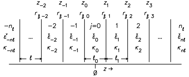
Similarly the $-z$ propagated reflection coefficient changes from $R_{\genfrac{}{}{0.0pt}{3}{\raisebox{-1.9pt}{\(\scriptscriptstyle s\)}}{\raisebox{1.9pt}{\(\scriptscriptstyle p\)}}-}[{\succ}z_{\jmath+1}]$ succeeding or just above the boundary between layers $\jmath+1$ to $\jmath$, to smaller $z$ down to the next boundary at $z_{\jmath}$, with the formula

with the interfacial reflections across the jump defined in (6), noting reversed signs for the reversed propagation direction in $z$ compared to Eq. (5).

The Fresnel reflection coefficients decrease exponentially in $+z$ from $R_{\genfrac{}{}{0.0pt}{3}{\raisebox{-1.9pt}{\(\scriptscriptstyle s\)}}{\raisebox{1.9pt}{\(\scriptscriptstyle p\)}}+}[{\succ}\genfrac{}{}{}{1}{-\ell_0}{2}]=(R_{\genfrac{}{}{0.0pt}{3}{\raisebox{-1.9pt}{\(\scriptscriptstyle s\)}}{\raisebox{1.9pt}{\(\scriptscriptstyle p\)}}+}[{\prec}\genfrac{}{}{}{1}{-\ell_0}{2}]+r_{\genfrac{}{}{0.0pt}{3}{\raisebox{-1.9pt}{\(\scriptscriptstyle s\)}}{\raisebox{1.9pt}{\(\scriptscriptstyle p\)}}0})/(1+R_{\genfrac{}{}{0.0pt}{3}{\raisebox{-1.9pt}{\(\scriptscriptstyle s\)}}{\raisebox{1.9pt}{\(\scriptscriptstyle p\)}}+}[{\prec}\genfrac{}{}{}{1}{-\ell}{2}]r_{\genfrac{}{}{0.0pt}{3}{\raisebox{-1.9pt}{\(\scriptscriptstyle s\)}}{\raisebox{1.9pt}{\(\scriptscriptstyle p\)}}0})$ just above the $z_{0}=\genfrac{}{}{}{1}{-\ell_0}{2}$ jump in Eq. (5), and in $-z$ from $R_{\genfrac{}{}{0.0pt}{3}{\raisebox{-1.9pt}{\(\scriptscriptstyle s\)}}{\raisebox{1.9pt}{\(\scriptscriptstyle p\)}}-}[{\prec}\genfrac{}{}{}{1}{\ell_0}{2}]=(R_{\genfrac{}{}{0.0pt}{3}{\raisebox{-1.9pt}{\(\scriptscriptstyle s\)}}{\raisebox{1.9pt}{\(\scriptscriptstyle p\)}}-}[{\succ}\genfrac{}{}{}{1}{\ell_0}{2}]-r_{\genfrac{}{}{0.0pt}{3}{\raisebox{-1.9pt}{\(\scriptscriptstyle s\)}}{\raisebox{1.9pt}{\(\scriptscriptstyle p\)}}1})/(1-R_{\genfrac{}{}{0.0pt}{3}{\raisebox{-1.9pt}{\(\scriptscriptstyle s\)}}{\raisebox{1.9pt}{\(\scriptscriptstyle p\)}}-}[{\succ}\genfrac{}{}{}{1}{\ell}{2}]r_{\genfrac{}{}{0.0pt}{3}{\raisebox{-1.9pt}{\(\scriptscriptstyle s\)}}{\raisebox{1.9pt}{\(\scriptscriptstyle p\)}}1})$ just below the $z_{1}=\genfrac{}{}{}{1}{\ell_0}{2}$ jump in Eq. (7). They vary across the middle layer $\genfrac{}{}{}{1}{-\ell_0}{2}<z<\genfrac{}{}{}{1}{\ell_0}{2}$ as

and in their product, the $z$ dependence vanishes

giving $\mathcal{R}_{\genfrac{}{}{0.0pt}{3}{\raisebox{-1.9pt}{\(\scriptscriptstyle s\)}}{\raisebox{1.9pt}{\(\scriptscriptstyle p\)}}}$ from (2) and a Casimir force $F$ from (1) or (4) independent of $z$ across a constant permittivity layer within jumps on either side. A constant ZP force across a uniform layer is a well-known property of ZP force solutions.

A three-layer stack has the Fresnel reflection coefficient $R_{\genfrac{}{}{0.0pt}{3}{\raisebox{-1.9pt}{\(\scriptscriptstyle s\)}}{\raisebox{1.9pt}{\(\scriptscriptstyle p\)}}+}[{\succ}\genfrac{}{}{}{1}{-\ell_0}{2}]=r_{\genfrac{}{}{0.0pt}{3}{\raisebox{-1.9pt}{\(\scriptscriptstyle s\)}}{\raisebox{1.9pt}{\(\scriptscriptstyle p\)}}0}$ above its lower jump at $z=\genfrac{}{}{}{1}{-\ell_0}{2}$, projecting with Eq. (5) from a uniform media everywhere below $R_{\genfrac{}{}{0.0pt}{3}{\raisebox{-1.9pt}{\(\scriptscriptstyle s\)}}{\raisebox{1.9pt}{\(\scriptscriptstyle p\)}}+}[z{<}\genfrac{}{}{}{1}{-\ell_0}{2}]=0$. It has the reflection coefficient $R_{\genfrac{}{}{0.0pt}{3}{\raisebox{-1.9pt}{\(\scriptscriptstyle s\)}}{\raisebox{1.9pt}{\(\scriptscriptstyle p\)}}-}[{\prec}\genfrac{}{}{}{1}{\ell_0}{2}]=-r_{\genfrac{}{}{0.0pt}{3}{\raisebox{-1.9pt}{\(\scriptscriptstyle s\)}}{\raisebox{1.9pt}{\(\scriptscriptstyle p\)}}1}$ below its upper jump at $z=\genfrac{}{}{}{1}{\ell_0}{2}$, projecting with (7) from a uniform media everywhere above $R_{\genfrac{}{}{0.0pt}{3}{\raisebox{-1.9pt}{\(\scriptscriptstyle s\)}}{\raisebox{1.9pt}{\(\scriptscriptstyle p\)}}-}[z{>}\genfrac{}{}{}{1}{\ell_0}{2}]=0$. Combining gives the product $R_{\genfrac{}{}{0.0pt}{3}{\raisebox{-1.9pt}{\(\scriptscriptstyle s\)}}{\raisebox{1.9pt}{\(\scriptscriptstyle p\)}}+}[z]R_{\genfrac{}{}{0.0pt}{3}{\raisebox{-1.9pt}{\(\scriptscriptstyle s\)}}{\raisebox{1.9pt}{\(\scriptscriptstyle p\)}}-}[z]=-r_{\genfrac{}{}{0.0pt}{3}{\raisebox{-1.9pt}{\(\scriptscriptstyle s\)}}{\raisebox{1.9pt}{\(\scriptscriptstyle p\)}}0}r_{\genfrac{}{}{0.0pt}{3}{\raisebox{-1.9pt}{\(\scriptscriptstyle s\)}}{\raisebox{1.9pt}{\(\scriptscriptstyle p\)}}1}\exp[-2\kappa_{0}\ell_{0}]$ in the middle layer $\genfrac{}{}{}{1}{-\ell_0}{2}<z<\genfrac{}{}{}{1}{\ell_0}{2}$ from (8). With (6), the product leads to the Lifshitz collaborative formula (Dzyaloshinskii et al., 1961, Eq. (4.14)).

A five-layer stack $n_{\ell}=2$ with layers of equal thicknesses $\ell$ counted $-2\leq j\leq 2$ has four contained jumps, at $z_{-1}=\genfrac{}{}{}{1}{-3\ell}{2}$, $z_{0}=\genfrac{}{}{}{1}{-\ell}{2}$, $z_{1}=\genfrac{}{}{}{1}{\ell}{2}$, and $z_{2}=\genfrac{}{}{}{1}{3\ell}{2}$ as in Figure 4. The Fresnel reflection coefficient in (8) comes from the $+z$ propagated coefficient just above the jump at $z_{-1}$, $R_{\genfrac{}{}{0.0pt}{3}{\raisebox{-1.9pt}{\(\scriptscriptstyle s\)}}{\raisebox{1.9pt}{\(\scriptscriptstyle p\)}}+}[{\succ}\genfrac{}{}{}{1}{-3\ell}{2}]=r_{\genfrac{}{}{0.0pt}{3}{\raisebox{-1.9pt}{\(\scriptscriptstyle s\)}}{\raisebox{1.9pt}{\(\scriptscriptstyle p\)}}-1}$, which gives $R_{\genfrac{}{}{0.0pt}{3}{\raisebox{-1.9pt}{\(\scriptscriptstyle s\)}}{\raisebox{1.9pt}{\(\scriptscriptstyle p\)}}+}[{\prec}\genfrac{}{}{}{1}{-\ell}{2}]=r_{\genfrac{}{}{0.0pt}{3}{\raisebox{-1.9pt}{\(\scriptscriptstyle s\)}}{\raisebox{1.9pt}{\(\scriptscriptstyle p\)}}-1}\exp[-2\kappa_{-1}\ell]$ just below the next jump at $z_{0}$, and then the needed $R_{\genfrac{}{}{0.0pt}{3}{\raisebox{-1.9pt}{\(\scriptscriptstyle s\)}}{\raisebox{1.9pt}{\(\scriptscriptstyle p\)}}+}[{\succ}\genfrac{}{}{}{1}{-\ell}{2}]$ across $z_{0}$ with $r_{\genfrac{}{}{0.0pt}{3}{\raisebox{-1.9pt}{\(\scriptscriptstyle s\)}}{\raisebox{1.9pt}{\(\scriptscriptstyle p\)}}0}$ using Eq. (5). Similarly the Fresnel reflection coefficient just below the jump at $z_{2}$, $R_{\genfrac{}{}{0.0pt}{3}{\raisebox{-1.9pt}{\(\scriptscriptstyle s\)}}{\raisebox{1.9pt}{\(\scriptscriptstyle p\)}}-}[{\prec}\genfrac{}{}{}{1}{3\ell}{2}]=-r_{\genfrac{}{}{0.0pt}{3}{\raisebox{-1.9pt}{\(\scriptscriptstyle s\)}}{\raisebox{1.9pt}{\(\scriptscriptstyle p\)}}2}$, is propagated in $-z$ to yield $R_{\genfrac{}{}{0.0pt}{3}{\raisebox{-1.9pt}{\(\scriptscriptstyle s\)}}{\raisebox{1.9pt}{\(\scriptscriptstyle p\)}}-}[{\succ}\genfrac{}{}{}{1}{\ell}{2}]=-r_{\genfrac{}{}{0.0pt}{3}{\raisebox{-1.9pt}{\(\scriptscriptstyle s\)}}{\raisebox{1.9pt}{\(\scriptscriptstyle p\)}}2}\exp[-2\kappa_{1}\ell]$ just above the next lower jump at $z_{1}$, and then the needed $R_{\genfrac{}{}{0.0pt}{3}{\raisebox{-1.9pt}{\(\scriptscriptstyle s\)}}{\raisebox{1.9pt}{\(\scriptscriptstyle p\)}}-}[{\prec}\genfrac{}{}{}{1}{\ell}{2}]$ below $z_{1}$ with $r_{\genfrac{}{}{0.0pt}{3}{\raisebox{-1.9pt}{\(\scriptscriptstyle s\)}}{\raisebox{1.9pt}{\(\scriptscriptstyle p\)}}1}$ using Eq. (7). The resulting product of reflection coefficients in Eq. (8) agrees with Zhou and Spruch (1995, Eqs. (3.12)–(3.16)).

Though changing symbols and formulae add serious complications, the Casimir force in (1) or (4) with any number of layers appears to be consistent with what is developed and discussed in numerous studies (Tomaš, 2002; Raabe et al., 2003; Henkel & Joulain, 2005; Ellingsen, 2007).

A sandwich of two identical layers around a middle layer $\jmath=0$ with permittivities $\check{\varepsilon}_{1}=\check{\varepsilon}_{-1}$ has jump coefficients $r_{\genfrac{}{}{0.0pt}{3}{\raisebox{-1.9pt}{\(\scriptscriptstyle s\)}}{\raisebox{1.9pt}{\(\scriptscriptstyle p\)}}0}=-r_{\genfrac{}{}{0.0pt}{3}{\raisebox{-1.9pt}{\(\scriptscriptstyle s\)}}{\raisebox{1.9pt}{\(\scriptscriptstyle p\)}}1}$, and so a product of reflection coefficients $R_{\genfrac{}{}{0.0pt}{3}{\raisebox{-1.9pt}{\(\scriptscriptstyle s\)}}{\raisebox{1.9pt}{\(\scriptscriptstyle p\)}}+}[z]R_{\genfrac{}{}{0.0pt}{3}{\raisebox{-1.9pt}{\(\scriptscriptstyle s\)}}{\raisebox{1.9pt}{\(\scriptscriptstyle p\)}}-}[z]=r_{\genfrac{}{}{0.0pt}{3}{\raisebox{-1.9pt}{\(\scriptscriptstyle s\)}}{\raisebox{1.9pt}{\(\scriptscriptstyle p\)}}0}^{2}\exp[-2\kappa_{0}\ell_{0}]>0$ or $\mathcal{R}_{\genfrac{}{}{0.0pt}{3}{\raisebox{-1.9pt}{\(\scriptscriptstyle s\)}}{\raisebox{1.9pt}{\(\scriptscriptstyle p\)}}}[z]>0$ from (2), meaning that the Casimir ZP force $F[z]$ defined in Eqs. (1) or (4) is negative or attractive. It can be seen too that recursive application of the formulae (5) and (7) in a spatially symmetric arrangement around a middle layer $\jmath=0$ with $\check{\varepsilon}_{\jmath}=\check{\varepsilon}_{-\jmath}$, for any number of layers even of varying thicknesses with $\ell_{\jmath}=\ell_{-\jmath}$, gives $R_{\genfrac{}{}{0.0pt}{3}{\raisebox{-1.9pt}{\(\scriptscriptstyle s\)}}{\raisebox{1.9pt}{\(\scriptscriptstyle p\)}}+}[{\succ}\genfrac{}{}{}{1}{-\ell_0}{2}]=R_{\genfrac{}{}{0.0pt}{3}{\raisebox{-1.9pt}{\(\scriptscriptstyle s\)}}{\raisebox{1.9pt}{\(\scriptscriptstyle p\)}}-}[{\prec}\genfrac{}{}{}{1}{\ell_0}{2}]$, and so in the middle layer $R_{\genfrac{}{}{0.0pt}{3}{\raisebox{-1.9pt}{\(\scriptscriptstyle s\)}}{\raisebox{1.9pt}{\(\scriptscriptstyle p\)}}+}[z]R_{\genfrac{}{}{0.0pt}{3}{\raisebox{-1.9pt}{\(\scriptscriptstyle s\)}}{\raisebox{1.9pt}{\(\scriptscriptstyle p\)}}-}[z]>0$, $\mathcal{R}_{\genfrac{}{}{0.0pt}{3}{\raisebox{-1.9pt}{\(\scriptscriptstyle s\)}}{\raisebox{1.9pt}{\(\scriptscriptstyle p\)}}}[z]>0$, and an attractive ZP force $F[z]<0$ (as in Lambrecht et al. 1997; Henkel & Joulain 2005). For a symmetric arrangement it also follows that $R_{\genfrac{}{}{0.0pt}{3}{\raisebox{-1.9pt}{\(\scriptscriptstyle s\)}}{\raisebox{1.9pt}{\(\scriptscriptstyle p\)}}+}[z]=R_{\genfrac{}{}{0.0pt}{3}{\raisebox{-1.9pt}{\(\scriptscriptstyle s\)}}{\raisebox{1.9pt}{\(\scriptscriptstyle p\)}}-}[-z]$ or $R_{\genfrac{}{}{0.0pt}{3}{\raisebox{-1.9pt}{\(\scriptscriptstyle s\)}}{\raisebox{1.9pt}{\(\scriptscriptstyle p\)}}+}[z]R_{\genfrac{}{}{0.0pt}{3}{\raisebox{-1.9pt}{\(\scriptscriptstyle s\)}}{\raisebox{1.9pt}{\(\scriptscriptstyle p\)}}-}[z]=R_{\genfrac{}{}{0.0pt}{3}{\raisebox{-1.9pt}{\(\scriptscriptstyle s\)}}{\raisebox{1.9pt}{\(\scriptscriptstyle p\)}}+}[-z]R_{\genfrac{}{}{0.0pt}{3}{\raisebox{-1.9pt}{\(\scriptscriptstyle s\)}}{\raisebox{1.9pt}{\(\scriptscriptstyle p\)}}-}[-z]$, giving $\mathcal{R}_{\genfrac{}{}{0.0pt}{3}{\raisebox{-1.9pt}{\(\scriptscriptstyle s\)}}{\raisebox{1.9pt}{\(\scriptscriptstyle p\)}}}[z]=\mathcal{R}_{\genfrac{}{}{0.0pt}{3}{\raisebox{-1.9pt}{\(\scriptscriptstyle s\)}}{\raisebox{1.9pt}{\(\scriptscriptstyle p\)}}}[-z]$, and so a symmetric ZP force $F[z]=F[-z]$ for all $z$.

In principle the $\omega$ integral in Eqs. (1) and (4) may be divergent, as the interfacial reflections $r_{p\jmath}$ from (6) do not vanish as $\omega\rightarrow\infty$, and these enter into the reflection coefficients $R_{p\pm}[z]$ and reflection term $\mathcal{R}_{p}$. However the attenuation factor $\exp[-2\kappa_{0}\ell_{0}]$, which multiplies the product of the reflection coefficients from the two nearest jumps in (8), does go to zero as $\omega$ goes to infinity for finite $\ell_{0}$, since $\kappa_{0}$ from Eq. (3) increases with $\omega$. Thus quantum divergences are not seen where the permittivity is constant across a finite layer.

For a three-layer stack, the ZP force integral Eq. (4) in a middle layer of thickness $\ell_{0}$ is conveniently rewritten in terms of a new dimensionless integration variable $\eta=\kappa_{0}\ell_{0}=(\check{\varepsilon}[\xi]\xi^{2}+\omega^{2})^{1/2}\ell_{0}/c$, which substitutes for the frequency $\omega$. Using the derivative $\partial\eta^{2}/\partial\omega^{2}=(\ell_{0}/c)^{2}$ or $\eta d\eta=(\ell_{0}/c)^{2}\omega d\omega$, reforms the $\omega$ integral into an integral in $\eta$ as

As described in Appendix B, for a small middle-layer thickness $\ell_{0}$, the $\eta$ integrand is determined by the product $\eta^{2}\exp[-2\eta]$, and the ZP force variation with $\ell_{0}$ follows the external factor $1/\ell_{0}^{3}$. The product $\eta^{2}\exp[-2\eta]$ has its maximum around $\eta=1$, corresponding to the wavenumber $\kappa_{0}=1/\ell_{0}$, and drops off exponentially beyond.

Other limiting forms arise when the middle-layer thickness is greater than a cross-over scale $\ell_{0}>\ell_{\pm}$, as most usually a $1/\ell_{0}^{4}$ ZP force retarded dependence as elaborated in Appendices A and B. Symmetric multilayer stacks exhibit the same asymptotic behavior as a three-layer stack, since ZP forces are determined in the nearest layers.

The definition for the ZP force from Eq. (1) should be applicable too in a stratified medium with a 1D smoothly varying complex permittivity $\varepsilon[z]$ or real $\check{\varepsilon}[z]$ and corresponding real $\kappa[z]$ defined by Eq. (3). In the limit that the layer thickness $\ell$ becomes infinitesimal, the Fresnel recursion formulae Eqs. (5) and (7) produce differential equations for a graded permittivity.

The expression for the reflection coefficient at the high $z$ end of the $\jmath=0$ interval $R_{\genfrac{}{}{0.0pt}{3}{\raisebox{-1.9pt}{\(\scriptscriptstyle s\)}}{\raisebox{1.9pt}{\(\scriptscriptstyle p\)}}\pm}[{\prec}\genfrac{}{}{}{1}{\ell}{2}]$ in terms of its value just below the low $z$ jump $R_{\genfrac{}{}{0.0pt}{3}{\raisebox{-1.9pt}{\(\scriptscriptstyle s\)}}{\raisebox{1.9pt}{\(\scriptscriptstyle p\)}}\pm}[{\prec}\genfrac{}{}{}{1}{-\ell}{2}]$ from Eq. (5), with the substitution of Taylor series’ in powers of $\ell$, $R_{\genfrac{}{}{0.0pt}{3}{\raisebox{-1.9pt}{\(\scriptscriptstyle s\)}}{\raisebox{1.9pt}{\(\scriptscriptstyle p\)}}+}[{\prec}\pm\genfrac{}{}{}{1}{\ell}{2}]=R_{\genfrac{}{}{0.0pt}{3}{\raisebox{-1.9pt}{\(\scriptscriptstyle s\)}}{\raisebox{1.9pt}{\(\scriptscriptstyle p\)}}+}[0]\pm({\partial R_{\genfrac{}{}{0.0pt}{3}{\raisebox{-1.9pt}{\(\scriptscriptstyle s\)}}{\raisebox{1.9pt}{\(\scriptscriptstyle p\)}}+}/\partial z})\genfrac{}{}{}{1}{\ell}{2}+\cdots$, $r_{\genfrac{}{}{0.0pt}{3}{\raisebox{-1.9pt}{\(\scriptscriptstyle s\)}}{\raisebox{1.9pt}{\(\scriptscriptstyle p\)}}0}=\rho_{\genfrac{}{}{0.0pt}{3}{\raisebox{-1.9pt}{\(\scriptscriptstyle s\)}}{\raisebox{1.9pt}{\(\scriptscriptstyle p\)}}}[-\genfrac{}{}{}{1}{\ell}{2}]\ell=\rho_{\genfrac{}{}{0.0pt}{3}{\raisebox{-1.9pt}{\(\scriptscriptstyle s\)}}{\raisebox{1.9pt}{\(\scriptscriptstyle p\)}}}[0]\ell-({\partial\rho_{\genfrac{}{}{0.0pt}{3}{\raisebox{-1.9pt}{\(\scriptscriptstyle s\)}}{\raisebox{1.9pt}{\(\scriptscriptstyle p\)}}}/\partial z})\ell^{2}/2+\cdots$, and $\exp[-2\kappa_{0}\ell]=1-2\kappa_{0}\ell+\cdots$, gives the differential equation for $R_{\genfrac{}{}{0.0pt}{3}{\raisebox{-1.9pt}{\(\scriptscriptstyle s\)}}{\raisebox{1.9pt}{\(\scriptscriptstyle p\)}}+}[z]$ around $z=0$

introducing the smoothly varying reflection $\rho_{\genfrac{}{}{0.0pt}{3}{\raisebox{-1.9pt}{\(\scriptscriptstyle s\)}}{\raisebox{1.9pt}{\(\scriptscriptstyle p\)}}}[z_{\jmath}]\equiv r_{\genfrac{}{}{0.0pt}{3}{\raisebox{-1.9pt}{\(\scriptscriptstyle s\)}}{\raisebox{1.9pt}{\(\scriptscriptstyle p\)}}\jmath}/\ell$, and keeping terms only to lowest order in $\ell$. The differential equation for $R_{\genfrac{}{}{0.0pt}{3}{\raisebox{-1.9pt}{\(\scriptscriptstyle s\)}}{\raisebox{1.9pt}{\(\scriptscriptstyle p\)}}-}[z]$ is contained in this equation also, which is found similarly by defining the reflection coefficient for the low $z$ end of the $\jmath=0$ interval $R_{\genfrac{}{}{0.0pt}{3}{\raisebox{-1.9pt}{\(\scriptscriptstyle s\)}}{\raisebox{1.9pt}{\(\scriptscriptstyle p\)}}-}[{\succ}\genfrac{}{}{}{1}{-\ell}{2}]$ in terms of its value just above the high $z$ jump $R_{\genfrac{}{}{0.0pt}{3}{\raisebox{-1.9pt}{\(\scriptscriptstyle s\)}}{\raisebox{1.9pt}{\(\scriptscriptstyle p\)}}-}[{\succ}\genfrac{}{}{}{1}{\ell}{2}]$ using Eq. (7), with the additional Taylor series’ $R_{\genfrac{}{}{0.0pt}{3}{\raisebox{-1.9pt}{\(\scriptscriptstyle s\)}}{\raisebox{1.9pt}{\(\scriptscriptstyle p\)}}-}[{\succ}\pm\genfrac{}{}{}{1}{\ell}{2}]=R_{\genfrac{}{}{0.0pt}{3}{\raisebox{-1.9pt}{\(\scriptscriptstyle s\)}}{\raisebox{1.9pt}{\(\scriptscriptstyle p\)}}-}[0]\pm({\partial R_{\genfrac{}{}{0.0pt}{3}{\raisebox{-1.9pt}{\(\scriptscriptstyle s\)}}{\raisebox{1.9pt}{\(\scriptscriptstyle p\)}}-}/\partial z})\genfrac{}{}{}{1}{\ell}{2}+\cdots$, and $r_{\genfrac{}{}{0.0pt}{3}{\raisebox{-1.9pt}{\(\scriptscriptstyle s\)}}{\raisebox{1.9pt}{\(\scriptscriptstyle p\)}}1}=\rho_{\genfrac{}{}{0.0pt}{3}{\raisebox{-1.9pt}{\(\scriptscriptstyle s\)}}{\raisebox{1.9pt}{\(\scriptscriptstyle p\)}}}[\genfrac{}{}{}{1}{\ell}{2}]\ell=\rho_{\genfrac{}{}{0.0pt}{3}{\raisebox{-1.9pt}{\(\scriptscriptstyle s\)}}{\raisebox{1.9pt}{\(\scriptscriptstyle p\)}}}[0]\ell+({\partial\rho_{\genfrac{}{}{0.0pt}{3}{\raisebox{-1.9pt}{\(\scriptscriptstyle s\)}}{\raisebox{1.9pt}{\(\scriptscriptstyle p\)}}}/\partial z})\ell^{2}/2+\cdots$. Though relations are derived for around $z=0$, they are applicable at all $z$ in the small $\ell$ limit for an infinite multilayer stack.

The smoothly varying reflection $\rho_{\genfrac{}{}{0.0pt}{3}{\raisebox{-1.9pt}{\(\scriptscriptstyle s\)}}{\raisebox{1.9pt}{\(\scriptscriptstyle p\)}}}[z_{\jmath}]\equiv r_{\genfrac{}{}{0.0pt}{3}{\raisebox{-1.9pt}{\(\scriptscriptstyle s\)}}{\raisebox{1.9pt}{\(\scriptscriptstyle p\)}}\jmath}/\ell$ is introduced as it remains well defined in the small $\ell$ limit. The wavenumber and permittivity first derivatives are taken to be the jump differences between layers normalized by the layer thickness $\ell$, as $\partial\kappa/\partial z=(\kappa_{0}-\kappa_{-1})/\ell$ and $\partial\check{\varepsilon}/\partial z=(\check{\varepsilon}_{0}-\check{\varepsilon}_{-1})/\ell$. Substituting into Eq. (6) with the values at $z=0$, $\kappa[0]=\kappa_{0}$ and $\check{\varepsilon}[0]=\check{\varepsilon}_{0}$, then yields around $z=0$

written for $\ell\rightarrow 0$, and again recognizing that the relations remain applicable at all $z$ in an infinite multilayer stack. The differential Eq. (10) with (11) agrees with evanescent solutions from different formulations for the propagation of waves in a stratified medium (e.g. see Jacobsson 1965, Eq. (2.37); Lekner 2016, Chapter 5; and references).

For everywhere-small reflection coefficients $|R_{\genfrac{}{}{0.0pt}{3}{\raisebox{-1.9pt}{\(\scriptscriptstyle s\)}}{\raisebox{1.9pt}{\(\scriptscriptstyle p\)}}\pm}[z]|\ll 1$, consistent with small-amplitude periodic permittivity variations on top of a constant permittivity background, Eq. (10) can be linearized, which provides the closed-form integral solution

where the function $\tilde{R}_{\genfrac{}{}{0.0pt}{3}{\raisebox{-1.9pt}{\(\scriptscriptstyle s\)}}{\raisebox{1.9pt}{\(\scriptscriptstyle p\)}}\pm}[z]$ represents a prior approximation to the propagated Fresnel reflection coefficient.

ZP forces in a medium of graded permittivity are studied by Fourier analysis supposing relatively small reflection coefficients, which gives a denominator near one in $\mathcal{R}_{\genfrac{}{}{0.0pt}{3}{\raisebox{-1.9pt}{\(\scriptscriptstyle s\)}}{\raisebox{1.9pt}{\(\scriptscriptstyle p\)}}}[z]$ from (2), and a ZP force from (4) well approximated as

The approximations used here are quantified in numerical calculations described in Section 4.

The Fourier transform of a repeating spatial profile of some repetition length $\lambda$ can be expanded in a discrete Fourier series in wavenumbers $n/\lambda$ cycles per cm for integer modes $n$, extending in principle from $-\infty<n<\infty$, written for the ZP force as

in Fourier modes $\bar{F}_{n}$, or similarly for the reflection coefficients $R_{\genfrac{}{}{0.0pt}{3}{\raisebox{-1.9pt}{\(\scriptscriptstyle s\)}}{\raisebox{1.9pt}{\(\scriptscriptstyle p\)}}\pm}[z]$ in modes $\bar{R}_{(\genfrac{}{}{0.0pt}{3}{\raisebox{-1.9pt}{\(\scriptscriptstyle s\)}}{\raisebox{1.9pt}{\(\scriptscriptstyle p\)}}\pm)n}$, or for the smoothly varying reflections $\rho_{\genfrac{}{}{0.0pt}{3}{\raisebox{-1.9pt}{\(\scriptscriptstyle s\)}}{\raisebox{1.9pt}{\(\scriptscriptstyle p\)}}}[z]$ in modes $\bar{\rho}_{\genfrac{}{}{0.0pt}{3}{\raisebox{-1.9pt}{\(\scriptscriptstyle s\)}}{\raisebox{1.9pt}{\(\scriptscriptstyle p\)}}n}$. The Fourier modes are Hermitian with $\bar{F}_{-n}=\bar{F}_{n}^{*}$ for a real function $F[z]$, or are real with $\bar{F}_{-n}=\bar{F}_{n}$ for a symmetric function around $z=0$, $F[z]=F[-z]$.

Substituting Fourier series’ for the variables transforms the differential Eq. (10) into the algebraic equation in Fourier modes

ignoring the square of the reflection coefficient, and spatial variations in the wavenumber $\kappa$. Solutions for the ZP force are found with $\kappa$ in Eq. (3) determined by a diverging frequency $\omega$, which is spatially constant.

With $\kappa$ greater than the largest significant wavenumbers $n/\lambda$ in the smoothly varying reflection, Eq. (15) gives the proportionality $\bar{R}_{(\genfrac{}{}{0.0pt}{3}{\raisebox{-1.9pt}{\(\scriptscriptstyle s\)}}{\raisebox{1.9pt}{\(\scriptscriptstyle p\)}}\pm)n}\sim\bar{\rho}_{\genfrac{}{}{0.0pt}{3}{\raisebox{-1.9pt}{\(\scriptscriptstyle s\)}}{\raisebox{1.9pt}{\(\scriptscriptstyle p\)}}n}/\kappa$ in every important Fourier mode $n$, which means spatial quantities similarly go as $R_{\genfrac{}{}{0.0pt}{3}{\raisebox{-1.9pt}{\(\scriptscriptstyle s\)}}{\raisebox{1.9pt}{\(\scriptscriptstyle p\)}}\pm}\sim\rho_{\genfrac{}{}{0.0pt}{3}{\raisebox{-1.9pt}{\(\scriptscriptstyle s\)}}{\raisebox{1.9pt}{\(\scriptscriptstyle p\)}}}/\kappa$, and the product of reflection coefficients as $R_{\genfrac{}{}{0.0pt}{3}{\raisebox{-1.9pt}{\(\scriptscriptstyle s\)}}{\raisebox{1.9pt}{\(\scriptscriptstyle p\)}}+}R_{\genfrac{}{}{0.0pt}{3}{\raisebox{-1.9pt}{\(\scriptscriptstyle s\)}}{\raisebox{1.9pt}{\(\scriptscriptstyle p\)}}-}\sim\rho_{\genfrac{}{}{0.0pt}{3}{\raisebox{-1.9pt}{\(\scriptscriptstyle s\)}}{\raisebox{1.9pt}{\(\scriptscriptstyle p\)}}}^{2}/\kappa^{2}$. From Eq. (11), $\rho_{s}\sim 1/\kappa^{2}$, and the product of reflection coefficients goes as $R_{s+}R_{s-}\sim 1/\kappa^{6}$. On the other hand, the first term in the smoothly varying reflection $\rho_{p}$ from Eq. (11) is independent of $\kappa$, which gives $R_{p+}R_{p-}\sim 1/\kappa^{2}$ asymptotically for large $\kappa$. All in all, the first term in $\rho_{p}$ leads to a linearly divergent $\omega$ integral in Eq. (13), whereas integrals of the other cross-product terms and of the product $R_{s+}R_{s-}$ are convergent, and can be ignored by comparison. Thus only the first term in the parallel smoothly varying reflection determines the ZP force

So, with a smoothly varying permittivity, the integral over $\omega$ in (13) is indeed divergent and feels its maximum contribution from frequencies $\omega$ approaching a cutoff $\omega_{\rm{x}}$. On the other hand, the Matsubara frequency $\xi$ has a limited range of significant contribution as the spatial derivative of the permittivity $\check{\varepsilon}$, and so the smoothly varying reflection $\rho_{p}[z]$ in Eq. (16), disappear well below any physically reasonable cutoff with $\xi\ll\omega_{\rm{x}}$, and with them the reflection coefficient $R_{p\pm}$ from the Fourier relation Eq. (15). Thus the wavenumber in (3) is well approximated as $\kappa=\omega/c$. This result is quite unlike what was found with a constant permittivity in a finite layer $\ell$ where the ZP force integral (9) has its maximum contribution around the relatively small wavenumber $\kappa=1/\ell$.

Expressing the permittivity as a Fourier series’ too, but in its logarithm

for complex coefficients $\mkern 3.0mu\overline{\mkern-3.0mu\{\ln\check{\varepsilon}\}\mkern-3.0mu}\mkern 3.0mu_{n}$, yields for the smoothly varying reflection from Eq. (16), and for the reflection coefficient from (15)

using $\kappa=\omega/c$. Substituting into the ZP force integral Eq. (13) with $R_{s\pm}=0$ and the Fourier series’ for the reflection coefficient $R_{p\pm}[z]$ in its modes $\bar{R}_{(p\pm)n}$ from Eq. (18), then gives a Fourier series for the ZP pressure Eq. (14) with the mode coefficients

where the sum over $\pm$ integers $q$ represents a convolution, which arises with the product of Fourier series’. The $\omega$ integral has a smooth Lorentzian cutoff around an upper limit $\omega_{\rm{x}}$ introduced with the inserted term in divisor $(1+(\omega/\omega_{\rm{x}})^{2})^{2}$, which imposes a form of covariant regularization (Feynman & Hibbs 1965, Section 9.6, after Eq. (9-89); Mandl & Shaw 2010, Section 9.2, Eq. (9.9)). The light wavelength for the cutoff is correspondingly $\lambda_{\rm{x}}=2\pi c/\omega_{\rm{x}}$.

All explicit dependencies upon the repetition scale $\lambda$ factor out of the $\omega$ integral, substituting for $\omega$ with a dimensionless $\hat{\omega}=\omega\lambda_{\rm{x}}/(\pi c)$, and for $n$ and $q$ with the scaled-down $\hat{n}=n\lambda_{\rm{x}}/\lambda$ and $\hat{q}=q\lambda_{\rm{x}}/\lambda$. The frequency ratio has the equivalences $\omega/\omega_{\rm{x}}=\lambda_{\rm{x}}/\lambda=\hat{\omega}/\hat{\omega}_{\rm{x}}$, where $\hat{\omega}_{\rm{x}}=\omega_{\rm{x}}\lambda_{\rm{x}}/(\pi c)=2$. With some rearranging, the ZP force mode becomes

with

The Fourier modes of the physical (real) quantities are Hermitian, $\bar{F}_{-n}=\bar{F}_{n}^{*}$ and $\mkern 3.0mu\overline{\mkern-3.0mu\{\ln\check{\varepsilon}\}\mkern-3.0mu}\mkern 3.0mu_{-n}=\mkern 3.0mu\overline{\mkern-3.0mu\{\ln\check{\varepsilon}\}\mkern-3.0mu}\mkern 3.0mu_{n}^{*}$, but the cutoff function $\mathfrak{C}$ is real, and does not change by taking the complex conjugate of Eq. (20), and so must remain unchanged with the equivalent flipping of the signs of both $n$ and $q$. It follows that the $\hat{\omega}$ frequency integrand in $\mathfrak{C}$ must also be unchanged with the change of sign $\hat{\omega}\rightarrow-\hat{\omega}$, which gives for the integral $\int_{-\infty}^{0}\cdots d\hat{\omega}=\int_{0}^{\infty}\cdots d\hat{\omega}$ as it appears in Eq. (21). The integral in the cutoff function is doubled as its domain is extended to span the full $\pm\hat{\omega}$ real axis. Looping over the upper (or equivalently lower) half complex $\hat{\omega}$ plane at infinity, which incurs no additional contribution, provides a contour in the continued $\hat{\omega}$ complex plane that encloses the $\hat{\omega}=2i$ Cauchy residue plus contained or overlapping residues for $\hat{n}-\hat{q}>0$ and $\hat{q}<0$. A real resultant for $\mathfrak{C}$ is found as shown in Figure 5, which ranges from 1 at the dc $\hat{n}-\hat{q}=\hat{q}=0$, diminishes for larger wavenumbers, and becomes slightly negative for $(\hat{n}-\hat{q})\hat{q}\lesssim-2$ beyond the zero contour (dotted). The resulting cutoff function $\mathfrak{C}$ is indeed symmetric with the simultaneous change of sign in $n$ and $q$.

The Fourier modes $\mkern 3.0mu\overline{\mkern-3.0mu\{\ln\check{\varepsilon}\}\mkern-3.0mu}\mkern 3.0mu_{n}$ for a given repeating waveform are independent of the wavelength $\lambda$, and so not changed with its rescaling. As long as the significant scales of variation in $\check{\varepsilon}[z]$ are large compared to the cutoff light wavelength $\lambda/n\gg\lambda_{\rm{x}}$, the integral can be treated as a constant $\mathfrak{C}=1$, giving a ZP force that decreases universally as the inverse square of the wavelength $1/\lambda^{2}$, from the external factor in Eq. (20). This ZP force property is validated in the numerical calculations for permittivity waves described in Section 4.

Even nonperiodic functional forms might be treated similarly approximated by discrete Fourier series’, like multiple discrete interacting shaped structures of varying separation. However an effectively changing Fourier profile with separation distance for structures of fixed cross section introduces some scale dependencies into the ZP force modes. Consideration of more general functions is outside the scope of the present analysis, which is mainly concerned with the properties of permittivity waves.

A high frequency cutoff is often used for divergent quantum integrals at extinction scales natural to the problem. Schwinger, DeRaad, and Milton (1978) introduce an atomic-scale cutoff in normally divergent integrals that arise in their formulation of the Casimir effect for interacting atoms, and reproduce reasonably well measured values of the surface tension and latent heat of vaporization in liquid He at 0K. Milonni and Lerner (1992) find that an atomic-scale cutoff is justified in microscopic atomic theories applying the Ewald-Oseen extinction theorem for interacting atoms.

Permittivity variations in acoustic waves are due to changes in electronic vibration or conductive electronic states, as elaborated in Appendix A, so a Compton-frequency cutoff seems appropriate for the problem $\omega_{\rm{x}}=\omega_{\rm{C}}=m_{\rm{e}}c^{2}/\hslash=7.7634$E20 rad/s, and is used for the calculations described in this paper. A Compton-frequency cutoff has been successfully applied with other ZP effects in electronic states, historically and most famously with the Lamb shift by Hans Bethe (Bethe 1947; Mandl & Shaw 2010, Section 9.6.2). The same cutoff is found using a quantum regularization procedure in a medium with a smoothly varying permittivity (Podgornik & Parsegian, 2004). QED calculations for electronic processes exhibit a small but finite correlation length corresponding to the Compton-scattering scale, which can be taken to arise due to the limited electron recoil from interactions with virtual photons by the small but finite electron inertia (Peskin & Schroeder 1995, Chapters 8-9; see also Cavalleri & Spavieri 1989).

Since permittivity variations in acoustic waves arise with electronic states, they should flatten out on a scale comparable to that of Compton electron-photon scattering since the material substance is actually represented by spatially discrete reradiating electronic oscillators. Where the permittivity is constant over a finite scale $\ell$, reflection coefficients become exponentially attenuated in frequency with their product going as $\exp[-2\omega\ell/c]$ as in Eq. (8) for a wavenumber $\kappa=\omega/c$, relevant for high-frequency processes. The ZP force $\omega$ integral Eq. (13) is governed by the weighting factor $\omega^{2}\exp[-2\omega\ell/c]$ near the high frequency cutoff, which peaks at $\omega=c/\ell$ and drops off exponentially beyond. With a scale for flattening somewhat less than the Compton scattering wavelength $\ell=\lambda_{\rm{C}}/(2\pi)$, where $\lambda_{\rm{C}}=h/(m_{\rm{e}}c)=2.4263$E${-}10$ cm, the integral of the weighting factor $\omega^{2}\exp[-2\omega\ell/c]$ out to $\omega\rightarrow\infty$ is close to the integral over $\omega^{2}$ alone sharply cut off at the Compton frequency $\omega_{\rm{C}}$, or the integral over $\omega^{2}$ with an imposed Lorentzian cutoff around $\omega_{\rm{C}}$ out to $\omega\rightarrow\infty$. It is known that retardation or dispersion can lead to a natural inherent quantum regularization (Horsley & Philbin, 2014).

Figure 6 shows an example ZP pressure profile $F[z]$ over one wavelength $\lambda$ in (a) due to a sinusoidal permittivity wave $\check{\varepsilon}[z]$ of representative wavelength and contrast (illustrated on top). The ZP pressure profile ranges from near zero to a maximum positive value for expansive in the most slopping portions of the permittivity wave.

For a permittivity variation symmetric about $z=0$, the Fourier modes $\mkern 3.0mu\overline{\mkern-3.0mu\{\ln\check{\varepsilon}\}\mkern-3.0mu}\mkern 3.0mu_{n}$ and correspondingly $\bar{F}_{n}$ are real with $\bar{F}_{-n}=\bar{F}_{n}$ in Eq. (20), giving the cosine series for $n\geq 0$ from Eq. (14)

with the logical $(n!=0)$, which is 1 on true and 0 on false, for double weight on all but the DC mode. Though most of the power in the profile (a) is in the bulk $\bar{F}_{0}$ and $\lambda/2$ $\bar{F}_{2}$ modes, a small residual containing mainly the $\bar{F}_{1}$ and $\bar{F}_{3}$ modes remains, which appears when the main ZP modes $\bar{F}_{0}$ and $\bar{F}_{2}$ are subtacted in (b). The subtraction is formulated strictly as $F[z]-\bar{F}_{0}-2\bar{F}_{2}\cos[4\pi z/\lambda]$, with $\bar{F}_{0}$ positive and $\bar{F}_{2}$ negative. The ZP force difference between normal and sign-reversed permittivity waves in (c) appears to be close to two times the residual in (b).

The ZP force model used for the figures is based on the Fourier decomposition from Section 3. The permittivity $\check{\varepsilon}[z]$ is defined by Eqs. (33) and (34) in Appendix A with a sinusoidal wave in one parameter as static permittivity $\varepsilon_{\rm{e}}=\langle\varepsilon_{\rm{e}}\rangle+\Delta\varepsilon_{\rm{e}}\cos 2\pi z/\lambda$, and the sign-reversed wave with $\cos\rightarrow-\cos$. The permittivity coefficients $\mkern 3.0mu\overline{\mkern-3.0mu\{\ln\check{\varepsilon}\}\mkern-3.0mu}\mkern 3.0mu_{n}$ in Eq. (18) are determined by expanding $\ln[\check{\varepsilon}[\cos[2\pi z/\lambda]]]$ as a series in cosine powers, then substituting with the exponential formula $\cos[2\pi z/\lambda]=(\exp[i2\pi z/\lambda]+1/\exp[i2\pi z/\lambda])/2$, and collecting common exponential powers algebraically using Mathematica (Wolfram, 1991). ZP force modes are then calculated using Eq. (20) with the integral in Matsubara frequency $\xi$ evaluated numerically. Both Mathematica and C++ were used in different formulations of the problem.

ZP pressure profiles for small amplitude permittivity waves all look qualitatively like the example shown here for $\Delta\varepsilon_{\rm{e}}/\langle\varepsilon_{\rm{e}}\rangle=0.1$ . They are dominated by the ZP modes $\bar{F}_{0}$ and $\bar{F}_{2}$. ZP pressure profiles for larger permittivity contrasts do noticeably change in appearance as illustrated in Figure 7 for $\Delta\varepsilon_{\rm{e}}/\langle\varepsilon_{\rm{e}}\rangle=0.5$. They exhibit an increased contribution from the ZP wave modes $\bar{F}_{1}$ and $\bar{F}_{3}$, with even a significant contribution from the $\bar{F}_{4}$ mode. For both figures, model parameters representative of quartz are used: electronic transition frequency $\omega_{\rm{e}}=2$E16 rad/s, plasma frequency $\omega_{\rm{p}}=0$, and mean static permittivity $\langle\varepsilon_{\rm{e}}\rangle=3.5$.

These ZP pressure profiles are in close quantitative agreement with those obtained by a direct method with the reflection coefficients evaluated by numerical integration of Eq. (12) iterating from a zero prior approximation, followed by numerical integration of the ZP force in Eq. (4) abruptly truncated at the Compton frequency $\omega_{\rm{x}}=\omega_{\rm{C}}$. The direct method provides reasonably indistinguishable results within its noise levels. However direct methods are more limited as they exhibit a noise cross-talk between Fourier modes close to the machine precision, which still becomes evident as systematic deviations in single high $n$ modes or in difference profiles.

Adding previous interations of the reflection coefficient $\tilde{R}$ back into the integral Eq. (12), even for permittivity waves as large as $\Delta\check{\varepsilon}=\langle\check{\varepsilon}\rangle$, introduces a change in the mode amplitudes $\bar{F}_{n}$ no larger than $2\%$ for the worst cases, at the smallest wavelengths $\lambda={\rm{E}}{-}9$ cm and in Fourier modes $n\gtrsim 30$. Introducing the denominator in the reflection terms produces relative changes of E$-6$ in the ZP force in the worst cases, and the perpendicular reflection terms $\mathcal{R}_{s}$ produce no larger than an E$-14$ relative effect. Little change in the profiles is seen at wavelengths near the cutoff, suggesting that the solution is little affected by the form of the cutoff as with the use of a Lorentzian cutoff in the Fourier method. In all of the numerical solutions described in this paper, integrals are evaluated using Simpson’s rule with at least 60 intervals over their ranges of maximum contribution. Increasing the number of intervals produces no significant changes ${>}1\%$ in the result. Inui (2008) has applied a direct computational implementation of a recursive formula for the reflection coefficients to estimate ZP pressures in linearly graded media.

In Figure 8, mode amplitudes $|2^{(n!=0)}\bar{F}_{n}|$ are shown for $\lambda={\rm{E}}{-}6.5$ cm, with a relative contrast of 0.5 in the four parameters, static permittivity $\varepsilon_{\rm{e}}$, electronic transition frequency $\omega_{\rm{e}}$, plasma frequency $\omega_{\rm{p}}$, and Drude collision frequency $\gamma_{\rm{D}}$. Characteristically $|\bar{F}_{0}|\simeq|2\bar{F}_{2}|$ and $|2\bar{F}_{1}|\simeq|2\bar{F}_{3}|$. Mode amplitudes drop off with a slope in $n$ beyond $n=3$ proportional to the relative contrast.

With the reversal in the sign of the permittivity wave, the main Fourier modes $\bar{F}_{0}$ and $\bar{F}_{2}$, with all of the even $n$ modes, do not change, and so vanish in the difference profile $\Delta F[z]$. Both of the next significant wave modes $\bar{F}_{1}$ and $\bar{F}_{3}$, as well as all of the odd $n$ modes, change sign, and so make up the difference profile $\Delta F[z]$.

References

- Auld (1973) Auld, B. 1973, Acoustic Fields and Waves in Solids, John Wiley & Sons, New York
- Bethe (1947) Bethe, H. A. 1947, The Electromagnetic Shift of Energy Levels, Phys. Rev., 72, 339–341, ADS
- Birkeland & Brevik (2007) Birkeland, O. J. & Brevik, I. 2007, Feigel effect: Extraction of momentum from vacuum?, Phys. Rev. E, 76(6), 066605, DOI, ADS
- Born & Wolf (1980) Born, M. & Wolf, E. 1980, Principles of Optics: Electromagnetic Theory of Propagation,Interference and Diffraction of Light, Pergamon Press, Oxford, 6th edition, ADS
- Caride et al. (2005) Caride, A. O., Klimchitskaya, G. L., Mostepanenko, V. M., & Zanette, S. I. 2005, Dependences of the van der Waals atom-wall interaction on atomic and material properties, Phys. Rev. A, 71(4), 042901, DOI, ADS
- Casimir (1948) Casimir, H. B. G. 1948, On the Attraction between Two Perfectly Conducting Plates, Proc. K. Ned. Akad. Wet., 51, 793–795
- Casimir & Polder (1948) Casimir, H. B. G. & Polder, D. 1948, The Influence of Retardation on the London-van der Waals Forces, Phys. Rev., 73, 360–372, DOI, ADS
- Cavalleri & Spavieri (1989) Cavalleri, G. & Spavieri, G. 1989, Friction in vacuo starting from eV, Nuovo Cimento A, 101, 213–223, DOI, ADS
- Cole & Puthoff (1993) Cole, D. C. & Puthoff, H. E. 1993, Extracting energy and heat from the vacuum, Phys. Rev. E, 48, 1562–1565, DOI, ADS
- Cooke (2007) Cooke, M. 2007, Filling the THz gap with new applications, Semiconductor Today, 2, 39–43
- Dowling (1989) Dowling, J. P. 1989, The Mathematics of the Casimir Effect, Math. Mag., 62, 324–331
- Dzyaloshinskii et al. (1961) Dzyaloshinskii, I. E., Lifshitz, E. M., & Pitaevskii, L. P. 1961, The general theory of van der Waals forces, Adv. Phys., 10, 165–209, DOI, ADS
- Ellingsen (2007) Ellingsen, S. A. 2007, Casimir attraction in multilayered plane parallel magnetodielectric systems, J. Phys. A, 40, 1951–1961, DOI, ADS
- Feigel (2004) Feigel, A. 2004, Quantum Vacuum Contribution to the Momentum of Dielectric Media, Phys. Rev. Lett., 92(2), 020404, DOI, ADS
- Feynman & Hibbs (1965) Feynman, R. P. & Hibbs, A. R. 1965, Quantum Mechanics and Path Integrals, McGraw Hill Book Company, New York
- Forward (1984) Forward, R. L. 1984, Extracting electrical energy from the vacuum by cohesion of charged foliated conductors, Phys. Rev. B, 30, 1700–1702, DOI, ADS
- Haisch & Moddel (2008) Haisch, B. & Moddel, G. 27 May, 2008, Quantum vacuum energy extraction, US Patent, 7,379,286
- Henkel & Joulain (2005) Henkel, C. & Joulain, K. 2005, Casimir force between designed materials: What is possible and what not, Europhys. Lett., 72, 929–935, DOI, ADS
- Horsley & Philbin (2014) Horsley, S. A. R. & Philbin, T. G. 2014, Canonical quantization of electromagnetism in spatially dispersive media, New J. Phys., 16(1), 013030, DOI, ADS
- Hough & White (1980) Hough, D. H. & White, R. A. 1980, The Calculation of Hamaker Constants from Lifshitz Theory with Applications to Wetting Phenomena, Adv. Colloid Interface Sci., 14, 3–14
- Ikeda (1990) Ikeda, T. 1990, Fundamentals of Piezoelectricity, Oxford Univ. Press, Oxford, New York, Tokyo
- Inui (2003) Inui, N. 2003, The Casimir Energy of a Medium Containing a Permittivity Gradient, J. Phys. Soc. Jpn., 72, 280–286, DOI, ADS
- Inui (2008) Inui, N. 2008, Casimir Energy of the Evanescent Field between Inhomogeneous Dielectric Slabs, J. Phys. Soc. Jpn., 77(8), 084001, DOI, ADS
- Jacobsson (1965) Jacobsson, R. 1965, Light Reflection from Films of Continuously Varying Refractive Index, in Progress in Optics, ed. E. Wolf, Vol. 5, J. Wiley and Sons, New York, 247–286
- Klimchitskaya et al. (2009) Klimchitskaya, G. L., Mohideen, U., & Mostepanenko, V. M. 2009, The Casimir force between real materials: Experiment and theory, Rev. Mod. Phys., 81, 1827–1885, DOI, ADS
- Lambrecht et al. (1997) Lambrecht, A., Jaekel, M., & Reynaud, S. 1997, The Casimir force for passive mirrors, Phys. Lett. A, 225, 188–194, DOI
- Lekner (2016) Lekner, J. 2016, Theory of Reflection: Reflection and Transmission of Electromagnetic, Particle and Acoustic Waves, Springer, Switzerland, 2nd edition
- Lifshitz (1956) Lifshitz, E. M. 1956, The Theory of Molecular Attractive Forces Between Solids, JETP, 2, 73–83, ADS
- Lipkin (1996) Lipkin, R. 1996, Thin-film mirror changes into a window, Science News, 149, 182, ADS
- Maclay (2000) Maclay, G. J. 2000, A design manual for micromachines using Casimir forces: Preliminary considerations, in Space Technology and Applications International Forum, ed. M. S. El-Genk, Vol. 504 of AIP Conference Series, AIP, Melville, New York, 1060–1065, DOI, ADS
- Mandl & Shaw (2010) Mandl, F. & Shaw, G. 2010, Quantum Field Theory, 2nd Edition, John Wiley & Sons, New York
- Mason (1966) Mason, W. 1966, Crystal Physics of Interaction Processes, Academic Press, New York, London
- Milonni (1994) Milonni, P. W. 1994, The Quantum Vacuum, An Introduction to Quantum Electrodynamics, Academic Press, Inc., San Diego, CA
- Milonni & Lerner (1992) Milonni, P. W. & Lerner, P. B. 1992, Extinction theorem, dispersion forces, and latent heat, Phys. Rev. A, 46, 1185–1193, DOI, ADS
- Ninham & Parsegian (1970) Ninham, B. W. & Parsegian, V. A. 1970, van der Waals Interactions in Multilayer Systems, J. Chem. Phys., 53, 3398–3402, DOI, ADS
- Peskin & Schroeder (1995) Peskin, M. E. & Schroeder, D. V. 1995, An Introduction to Quantum Field Theory, Perseus Books, New York
- Philbin et al. (2010) Philbin, T. G., Xiong, C., & Leonhardt, U. 2010, Casimir stress in an inhomogeneous medium, Ann. Phys. (N.Y.), 325, 579–595, DOI, ADS
- Pinto (1999) Pinto, F. 1999, Engine cycle of an optically controlled vacuum energy transducer, Phys. Rev. B, 60, 14740–14755, DOI, ADS
- Pinto (2008) Pinto, F. 2008, Membrane Nano-Actuation by Light-Driven Manipulation of van der Waals Forces: A Progress Report, in Space Technology and Applications International Forum-STAIF, ed. M. S. El-Genk, Vol. 969 of AIP Conference Series, AIP, Melville, New York, 1111–1119, DOI, ADS
- Podgornik et al. (2003) Podgornik, R., Hansen, P. L., & Parsegian, V. A. 2003, On a reformulation of the theory of Lifshitz-van der Waals interactions in multilayered systems, J. Chem. Phys., 119, 1070–1077, DOI, ADS
- Podgornik & Parsegian (2004) Podgornik, R. & Parsegian, V. A. 2004, Van der Waals interactions in a dielectric with continuously varying dielectric function, J. Chem. Phys., 121, 7467–7473, DOI, ADS
- Raabe et al. (2003) Raabe, C., Knöll, L., & Welsch, D. G. 2003, Three-dimensional Casimir force between absorbing multilayer dielectrics, Phys. Rev. A, 68(3), 033810, DOI, ADS
- Schwinger et al. (1978) Schwinger, J., DeRaad, Jr., L. L., & Milton, K. A. 1978, Casimir effect in dielectrics, Ann. Phys. (N.Y.), 115, 1–23, DOI, ADS
- Tomaš (2002) Tomaš, M. S. 2002, Casimir force in absorbing multilayers, Phys. Rev. A, 66(5), 052103, DOI, ADS
- Wang et al. (2007) Wang, X., Song, J., Liu, J., & Wang, Z. L. 2007, Direct-Current Nanogenerator Driven by Ultrasonic Waves, Science, 316, 102–105, DOI, ADS
- Wolfram (1991) Wolfram, S. 1991, Mathematica: a system for doing mathematics by computer, 2nd edition, Addison-Wesley Publishing Co. Inc., Advanced Book Program, Reading, MA, ADS
- Zhou & Spruch (1995) Zhou, F. & Spruch, L. 1995, van der Waals and retardation (Casimir) interactions of an electron or an atom with multilayered walls, Phys. Rev. A, 52, 297–310, DOI, ADS