Interference Channel with State Information

Lili Zhang Jinhua Jiang and Shuguang Cui ^†^†thanks: L. Zhang and S. Cui are with the Department of Electrical and Computer Engineering, Texas A$&$M University, College Station, TX 77843 USA (e-mail: lily.zhang@tamu.edu; cui@ece.tamu.edu).^†^†thanks: J. Jiang is with the Department of Electrical Engineering, Stanford University, Stanford, CA 94305 USA (email: jhjiang@stanford.edu).

Abstract

In this paper, we study the state-dependent two-user interference channel, where the state information is non-causally known at both transmitters but unknown to either of the receivers. We first propose two coding schemes for the discrete memoryless case: simultaneous encoding for the sub-messages in the first one and superposition encoding in the second one, both with rate splitting and Gel’fand-Pinsker coding. The corresponding achievable rate regions are established. Moreover, for the Gaussian case, we focus on the simultaneous encoding scheme and propose an active interference cancellation mechanism, which is a generalized dirty-paper coding technique, to partially eliminate the state effect at the receivers. The corresponding achievable rate region is then derived. We also propose several heuristic schemes for some special cases: the strong interference case, the mixed interference case, and the weak interference case. For the strong and mixed interference case, numerical results are provided to show that active interference cancellation significantly enlarges the achievable rate region. For the weak interference case, flexible power splitting instead of active interference cancellation improves the performance significantly.

I Introduction

The interference channel (IC) models the situation where several independent transmitters communicate with their corresponding receivers simultaneously over a common spectrum. Due to the shared medium, each receiver suffers from interferences caused by the transmissions of other transceiver pairs. The research of IC was initiated by Shannon [1] and the channel was first thoroughly studied by Ahlswede [2]. Later, Carleial [3] established an improved achievable rate region by applying the superposition coding scheme. In [4], Han and Kobayashi obtained the best achievable rate region known to date for the general IC by utilizing simultaneous decoding at the receivers. Recently, this rate region has been re-characterized with superposition encoding for the sub-messages [5, 6]. However, the capacity region of the general IC is still an open problem [4].

The capacity region for the corresponding Gaussian case is also unknown except for several special cases, such as the strong Gaussian IC and the very strong Gaussian IC [8, 7]. In addition, Sason [9] characterized the sum capacity for a special case of the Gaussian IC called the degraded Gaussian IC. For more general cases, Han-Kobayashi region [4] is still the best achievable rate region known to date. However, for the general Gaussian interference channel, the calculation of the Han-Kobayashi region bears high complexity. The authors in [10] proposed a simpler heuristic coding scheme, for which they set the private message power at both transmitters in a special way such that the interfered private signal-to-noise ratio (SNR) at each receiver is equal to $1$ . An upper bound on the capacity was also derived in [10] and it was shown that the gap between the heuristic lower bound and the capacity upper bound is less than one bit for both weak and mixed interference cases.

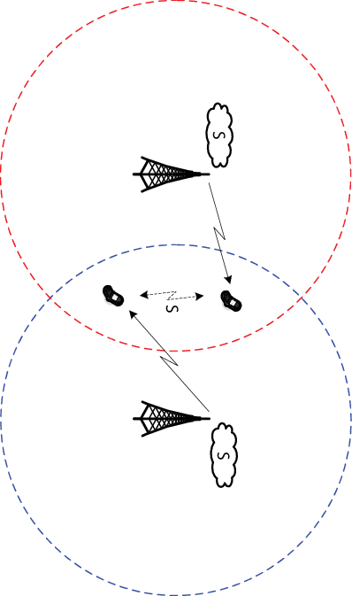
Many variations of the interference channel have also been studied, including the IC with feedback [11] and the IC with conferencing encoders/decoders [12]. Here, we study another variation of the IC: the state-dependent two-user IC with state information non-causally known at both transmitters. This situation may arise in a multi-cell downlink communication scenario as shown in Fig. 1, where two interested cells are interfering with each other and the mobiles suffer from some common interference (which can be from other neighboring cells and viewed as state) non-causally known at both of the two base-stations via certain collaboration with the neighboring base-station. Notably, communication over state-dependent channels has drawn lots of attentions due to its wide applications such as information embedding [13] and computer memories with defects [14]. The corresponding framework was also initiated by Shannon in [15], which established the capacity of a state-dependent discrete memoryless (DM) point-to-point channel with causal state information at the transmitter. In [16], Gel’fand and Pinsker obtained the capacity for such a point-to-point case with the state information non-causally known at the transmitter. Subsequently, Costa [17] extended Gel’fand-Pinsker coding to the state-dependent additive white Gaussian noise (AWGN) channel, where the state is an additive zero-mean Gaussian interference. This result is known as the dirty-paper coding (DPC) technique, which achieves the capacity as if there is no such an interference. For the multi-user case, extensions of the afore-mentioned schemes appeared in [18, 21, 19, 20] for the multiple access channel (MAC), the broadcast channel, and the degraded Gaussian relay channel, respectively.

In this paper, we study the state-dependent IC with state information non-causally known at the transmitters and develop two coding schemes, both of which jointly apply rate splitting and Gel’fand-Pinsker coding. In the first coding scheme, we deploy simultaneous encoding for the sub-messages, and in the second one, we deploy superposition encoding for the sub-messages. The associated achievable rate regions are derived based on the respective coding schemes. Then we specialize the achievable rate region corresponding to the simultaneous encoding scheme in the Gaussian case, where the common additive state is a zero-mean Gaussian random variable. Specifically, we introduce the notion of active interference cancellation, which generalizes dirty-paper coding by utilizing some transmitting power to partially cancel the common interference at both receivers. Furthermore, we propose heuristic schemes for the strong Gaussian IC, the mixed Gaussian IC, and the weak Gaussian IC with state information, respectively. For the strong Gaussian IC with state information, the transmitters only send common messages and the DPC parameters are optimized for one of the two resulting MACs. For the mixed Gaussian IC with state information, one transmitter sends common message and the other one sends private message, with DPC parameters optimized only for one receiver. For the weak interference case, we apply rate splitting, set the private message power at both transmitters to have the interfered private SNR at each receiver equal to $1$ [10], utilize sequential decoding, and optimize the DPC parameters for one of the MACs. The time-sharing technique is applied in all the three cases to obtain enlarged achievable rate regions. Numerical comparisons among the achievable rate regions and the capacity outer bound are also provided. For the strong and mixed interference cases, we show that the active interference cancellation mechanism improves the performance significantly; for the weak interference case, it is flexible power allocation instead of active interference cancellation that enlarges the achievable rate region significantly.

The rest of the paper is organized as follows. The channel model and the definition of achievable rate region are presented in Section II. In Section III, we provide two achievable rate regions for the discrete memoryless IC with state information non-causally known at both transmitters, based on the two different coding schemes, respectively. In Section IV, we discuss the Gaussian case and present the main idea of active interference cancellation. The strong interference, mixed interference, and weak interference cases are studied in Section V, VI, and VII, respectively. In Section VIII, numerical results comparing different inner bounds against the outer bound are given. Finally, we conclude the paper in Section IX.

Refer to caption — Fig. 1: A multi-cell downlink communication example, which can be modeled as an interference channel with state information non-causally known at both transmitters.

II Channel Model

Consider the interference channel as shown in Fig. 2, where two transmitters communicate with the corresponding receivers through a common medium that is dependent on state $S$ . The transmitters do not cooperate with each other; however, they both know the state information $S$ non-causally, which is known to neither of the receivers. Each receiver needs to decode the information from the corresponding transmitter.

II-A Discrete Memoryless Case

We use the following notations for the DM channel. The random variable is defined as $X$ with value $x$ in a finite set $\mathcal{X}$ . Let $p_{X}(x)$ be the probability mass function of $X$ on $\mathcal{X}$ . The corresponding sequences are denoted by $x^{n}$ with length $n$ .

The state-dependent two-user interference channel is defined by $(\mathcal{X}_{1},\mathcal{X}_{2},\mathcal{Y}_{1},\mathcal{Y}_{2},\mathcal{S},p(y_{1},y_{2}|x_{1},x_{2},s))$ , where $\mathcal{X}_{1},\mathcal{X}_{2}$ are two input alphabet sets, $\mathcal{Y}_{1},\mathcal{Y}_{2}$ are the corresponding output alphabet sets, $\mathcal{S}$ is the state alphabet set, and $p(y_{1},y_{2}|x_{1},x_{2},s)$ is the conditional probability of $(y_{1},y_{2})\in\mathcal{Y}_{1}\mathcal{\times}\mathcal{Y}_{2}$ given $(x_{1},x_{2},s)\in\mathcal{X}_{1}\mathcal{\times}\mathcal{X}_{2}\mathcal{\times}\mathcal{S}$ . The channel is assumed to be memoryless, i.e.,

p(y_{1}^{n},y_{2}^{n}|x_{1}^{n},x_{2}^{n},s^{n})=\prod_{i=1}^{n}p(y_{1i},y_{2i}|x_{1i},x_{2i},s_{i}),

where $i$ is the element index for each sequence.

A $(2^{nR_{1}},2^{nR_{2}},n)$ code for the above channel consists of two independent message sets $\{1,2,\cdots,2^{nR_{1}}\}$ and $\{1,2,\cdots,2^{nR_{2}}\}$ , two encoders that respectively assign two codewords to messages $m_{1}\in\{1,2,\cdots,2^{nR_{1}}\}$ and $m_{2}\in\{1,2,\cdots,2^{nR_{2}}\}$ based on the non-causally known state information $s^{n}$ , and two decoders that respectively determine the estimated messages $\hat{m}_{1}$ and $\hat{m}_{2}$ or declare an error from the received sequences.

The average probability of error is defined as:

P_{e}^{(n)}=\frac{1}{2^{n(R_{1}+R_{2})}}\sum_{m_{1},m_{2}}\textrm{Pr}\{\hat{m}_{1}\neq m_{1}\textrm{ or }\hat{m}_{2}\neq m_{2}|(m_{1},m_{2})\textrm{ is sent}\},

(1)

where $(m_{1},m_{2})$ is assumed to be uniformly distributed over $\{1,2,\cdots,2^{nR_{1}}\}\times\{1,2,\cdots,2^{nR_{2}}\}$ .

Definition 1.

A rate pair $(R_{1},R_{2})$ of non-negative real values is achievable if there exists a sequence of $(2^{nR_{1}},2^{nR_{2}},n)$ codes with $P_{e}^{(n)}\to 0$ as $n\to\infty$ . The set of all achievable rate pairs is defined as the capacity region.

II-B Gaussian Case

The Gaussian counterpart of the previously defined DM channel is shown in Fig. 3, where two transmitters communicate with the corresponding receivers through a common channel that is dependent on state $S$ , which can be treated as a common interference. The corresponding signal structure can be described by the following channel input and output relationship:

	$\displaystyle Y_{1}^{\prime}$	$\displaystyle=$	$\displaystyle h_{11}X_{1}^{\prime}+h_{12}X_{2}^{\prime}+S+Z_{1}^{\prime},$
	$\displaystyle Y_{2}^{\prime}$	$\displaystyle=$	$\displaystyle h_{22}X_{2}^{\prime}+h_{21}X_{1}^{\prime}+S+Z_{2}^{\prime},$

where $h_{ij}$ is the real link amplitude gain from the $j$ th transmitter to the $i$ th receiver, $X_{i}^{\prime}$ and $Y_{i}^{\prime}$ are the channel input and output, respectively, and $Z_{i}^{\prime}$ is the zero-mean AWGN noise with variance $N_{i}$ , for $i=1,2$ and $j=1,2$ . Both receivers also suffer from a zero-mean additive white Gaussian interference $S$ with variance $K$ , which is non-causally known at both transmitters¹¹ 1 In general, the additive states over the two links may not be the same, i.e., we may have $Y_{1}^{\prime}=h_{11}X_{1}^{\prime}+h_{12}X_{2}^{\prime}+S_{1}+Z_{1}^{\prime}$ and $Y_{2}^{\prime}=h_{22}X_{2}^{\prime}+h_{21}X_{1}^{\prime}+S_{2}+Z_{2}^{\prime}$ . However, in this paper we only focus on the simplest scenario: $S_{1}=S_{2}=S$ . The more general cases with state $(S_{1},S_{2})$ and different knowledge levels at the two transmitters will be studied in our future work.. Note that for this AWGN model, all the random variables are defined over the field of real numbers $\mathbb{R}$ .

Without loss of generality, we transform the signal model into the following standard form [4]:

	$\displaystyle Y_{1}$	$\displaystyle=$	$\displaystyle X_{1}+\sqrt{g_{12}}X_{2}+\frac{1}{\sqrt{N_{1}}}S+Z_{1},$		(2)
	$\displaystyle Y_{2}$	$\displaystyle=$	$\displaystyle X_{2}+\sqrt{g_{21}}X_{1}+\frac{1}{\sqrt{N_{2}}}S+Z_{2},$		(3)

where

	$\displaystyle Y_{1}$	$\displaystyle=$	$\displaystyle\frac{Y_{1}^{\prime}}{\sqrt{N_{1}}},\ X_{1}=\frac{h_{11}X_{1}^{\prime}}{\sqrt{N_{1}}},\ g_{12}=\frac{h_{12}^{2}N_{2}}{h_{22}^{2}N_{1}},\ Z_{1}=\frac{Z_{1}^{\prime}}{\sqrt{N_{1}}},$
	$\displaystyle Y_{2}$	$\displaystyle=$	$\displaystyle\frac{Y_{2}^{\prime}}{\sqrt{N_{2}}},\ X_{2}=\frac{h_{22}X_{2}^{\prime}}{\sqrt{N_{2}}},\ g_{21}=\frac{h_{21}^{2}N_{1}}{h_{11}^{2}N_{2}},\ Z_{2}=\frac{Z_{2}^{\prime}}{\sqrt{N_{2}}}.$

Note that $Z_{1}$ and $Z_{2}$ have unit variance in (2) and (3). We also impose the following power constraints on the channel inputs $X_{1}$ and $X_{2}$ :

\frac{1}{n}\sum_{i=1}^{n}(X_{1i})^{2}\leq P_{1},\textrm{ and }\frac{1}{n}\sum_{i=1}^{n}(X_{2i})^{2}\leq P_{2}.

III Achievable Rate Regions for DM Interference Channel with State Information

In this section, we propose two new coding schemes for the DM interference channel with state information non-causally known at both transmitters and quantify the associated achievable rate regions. For both coding schemes, we jointly deploy rate splitting and Gel’fand-Pinsker coding. Specifically, in the first coding scheme, we use simultaneous encoding on the sub-messages, while in the second one we apply superposition encoding.

III-A Coding Scheme I: Simultaneous Encoding

Now we introduce the following rate region achieved by the first coding scheme, which combines rate splitting and Gel’fand-Pinsker coding. Let us consider the auxiliary random variables $Q$ , $U_{1}$ , $V_{1}$ , $U_{2}$ , and $V_{2}$ , defined on arbitrary finite sets $\mathcal{Q}$ , $\mathcal{U}_{1}$ , $\mathcal{V}_{1}$ , $\mathcal{U}_{2}$ , and $\mathcal{V}_{2}$ , respectively. The joint probability distribution of the above auxiliary random variables and the state variable $S$ is chosen to satisfy the form $p(s)p(q)p(u_{1}|q,s)p(v_{1}|q,s)p(u_{2}|q,s)p(v_{2}|q,s)$ . Moreover, for a given $Q$ , we let the channel input $X_{j}$ be an arbitrary deterministic function of $U_{j}$ , $V_{j}$ , and $S$ . The achievable rate region of the simultaneous encoding scheme is given in the following theorem.

Theorem 1.

For a fixed probability distribution $p(q)p(u_{1}|q,s)p(v_{1}|q,s)p(u_{2}|q,s)p(v_{2}|q,s)$ , let $\mathcal{R}_{1}$ be the set of all non-negative rate tuple $(R_{10},R_{11},R_{20},R_{22})$ satisfying

$\displaystyle R_{11}$	$\displaystyle\leq$	$\displaystyle I(U_{1};U_{2}\|Q)+I(U_{1},U_{2};V_{1}\|Q)+I(V_{1};Y_{1}\|U_{1},U_{2},Q)-I(V_{1};S\|Q),$	(4)
$\displaystyle R_{10}$	$\displaystyle\leq$	$\displaystyle I(U_{1};U_{2}\|Q)+I(U_{1},U_{2};V_{1}\|Q)+I(U_{1};Y_{1}\|V_{1},U_{2},Q)-I(U_{1};S\|Q),$	(5)
$\displaystyle R_{10}+R_{11}$	$\displaystyle\leq$	$\displaystyle I(U_{1};U_{2}\|Q)+I(U_{1},U_{2};V_{1}\|Q)+I(U_{1},V_{1};Y_{1}\|U_{2},Q)-I(U_{1};S\|Q)-I(V_{1};S\|Q),$	(6)
$\displaystyle R_{11}+R_{20}$	$\displaystyle\leq$	$\displaystyle I(U_{1};U_{2}\|Q)+I(U_{1},U_{2};V_{1}\|Q)+I(V_{1},U_{2};Y_{1}\|U_{1},Q)-I(V_{1};S\|Q)-I(U_{2};S\|Q),$	(7)
$\displaystyle R_{10}+R_{20}$	$\displaystyle\leq$	$\displaystyle I(U_{1};U_{2}\|Q)+I(U_{1},U_{2};V_{1}\|Q)+I(U_{1},U_{2};Y_{1}\|V_{1},Q)-I(U_{1};S\|Q)-I(U_{2};S\|Q),$	(8)
$\displaystyle R_{10}+R_{11}+R_{20}$	$\displaystyle\leq$	$\displaystyle I(U_{1};U_{2}\|Q)+I(U_{1},U_{2};V_{1}\|Q)+I(U_{1},V_{1},U_{2};Y_{1}\|Q)-I(U_{1};S\|Q)-I(V_{1};S\|Q)-I(U_{2};S\|Q),$	(9)
$\displaystyle R_{22}$	$\displaystyle\leq$	$\displaystyle I(U_{2};U_{1}\|Q)+I(U_{2},U_{1};V_{2}\|Q)+I(V_{2};Y_{2}\|U_{2},U_{1},Q)-I(V_{2};S\|Q),$	(10)
$\displaystyle R_{20}$	$\displaystyle\leq$	$\displaystyle I(U_{2};U_{1}\|Q)+I(U_{2},U_{1};V_{2}\|Q)+I(U_{2};Y_{2}\|V_{2},U_{1},Q)-I(U_{2};S\|Q),$	(11)
$\displaystyle R_{20}+R_{22}$	$\displaystyle\leq$	$\displaystyle I(U_{2};U_{1}\|Q)+I(U_{2},U_{1};V_{2}\|Q)+I(U_{2},V_{2};Y_{2}\|U_{1},Q)-I(U_{2};S\|Q)-I(V_{2};S\|Q),$	(12)
$\displaystyle R_{22}+R_{10}$	$\displaystyle\leq$	$\displaystyle I(U_{2};U_{1}\|Q)+I(U_{2},U_{1};V_{2}\|Q)+I(V_{2},U_{1};Y_{2}\|U_{2},Q)-I(V_{2};S\|Q)-I(U_{1};S\|Q),$	(13)
$\displaystyle R_{20}+R_{10}$	$\displaystyle\leq$	$\displaystyle I(U_{2};U_{1}\|Q)+I(U_{2},U_{1};V_{2}\|Q)+I(U_{2},U_{1};Y_{2}\|V_{2},Q)-I(U_{2};S\|Q)-I(U_{1};S\|Q),$	(14)
$\displaystyle R_{20}+R_{22}+R_{10}$	$\displaystyle\leq$	$\displaystyle I(U_{2};U_{1}\|Q)+I(U_{2},U_{1};V_{2}\|Q)+I(U_{2},V_{2},U_{1};Y_{2}\|Q)-I(U_{2};S\|Q)-I(V_{2};S\|Q)-I(U_{1};S\|Q).$	(15)

Then for any $(R_{10},R_{11},R_{20},R_{22})\in\mathcal{R}_{1}$ , the rate pair $(R_{10}+R_{11},R_{20}+R_{22})$ is achievable for the DM interference channel with state information defined in Section II.

Remark 1.

The detailed proof is given in Appendix A with the outline sketched as follows. For the coding scheme in Theorem 1, the message at transmitter $j$ ( $j=1$ or $2$ ) is splitted into two parts: the public message $m_{j0}$ and the private message $m_{jj}$ . Furthermore, Gel’fand-Pinsker coding is utilized to help both transmitters send the messages with the non-causal knowledge of the state information. Specifically, transmitter $j$ finds the corresponding public codeword $u_{j}$ and the private codeword $v_{j}$ such that they are jointly typical with the state $s^{n}$ . Then the transmitting codeword is constructed as a deterministic function of the public codeword $u_{j}$ , the private codeword $v_{j}$ , and the state $s^{n}$ . At the receiver side, decoder $j$ tries to decode the corresponding messages from transmitter $j$ and the public message of the interfering transmitter. The rest follows by the usual error event grouping and error probability analysis.

Remark 2.

The auxiliary random variables in Theorem 1 can be interpreted as follows: $Q$ is the time-sharing random variable; $U_{j}$ and $V_{j}$ ( $j=1$ or $2$ ) are the auxiliary random variables to carry the public and private messages at transmitter $j$ , respectively. It can be easily seen from the joint probability distribution that $U_{j}$ and $V_{j}$ are conditionally independent given $Q$ and $S$ , which means that the public and private messages are encoded “simultaneously”.

An explicit description of the achievable rate region can be obtained by applying the Fourier-Motzkin algorithm [5] on our implicit description (4)-(15), as shown in the next corollary.

Corollary 1.

For a fixed probability distribution $p(q)p(u_{1}|q,s)p(v_{1}|q,s)p(u_{2}|q,s)p(v_{2}|q,s)$ , let $\hat{\mathcal{R}}_{1}$ be the set of all non-negative rate pairs $(R_{1},R_{2})$ satisfying

$\displaystyle R_{1}$	$\displaystyle\leq$	$\displaystyle\min\{d_{1},g_{1},a_{1}+b_{1},a_{1}+f_{1},a_{1}+e_{2},a_{1}+f_{2},b_{1}+e_{1},e_{1}+f_{1},e_{1}+f_{2}\},$	(16)
$\displaystyle R_{2}$	$\displaystyle\leq$	$\displaystyle\min\{d_{2},g_{2},a_{2}+b_{2},a_{2}+f_{2},a_{2}+e_{1},a_{2}+f_{1},b_{2}+e_{2},e_{2}+f_{2},e_{2}+f_{1}\},$	(17)
$\displaystyle R_{1}+R_{2}$	$\displaystyle\leq$	$\displaystyle\min\{a_{1}+g_{2},a_{2}+g_{1},e_{1}+g_{2},e_{2}+g_{1},e_{1}+e_{2},a_{1}+a_{2}+f_{1},a_{1}+a_{2}+f_{2},a_{1}+b_{2}+e_{2},a_{2}+b_{1}+e_{1}\},$	(18)
$\displaystyle R_{1}+2R_{2}$	$\displaystyle\leq$	$\displaystyle\min\{e_{1}+f_{1}+2a_{2},e_{1}+2a_{2}+f_{2},e_{1}+a_{2}+g_{2}\},$	(19)
$\displaystyle 2R_{1}+R_{2}$	$\displaystyle\leq$	$\displaystyle\min\{e_{2}+f_{2}+2a_{1},e_{2}+2a_{1}+f_{1},e_{2}+a_{1}+g_{1}\},$	(20)

where

$\displaystyle a_{1}$	$\displaystyle=$	$\displaystyle I(U_{1};U_{2}\|Q)+I(U_{1},U_{2};V_{1}\|Q)+I(V_{1};Y_{1}\|U_{1},U_{2},Q)-I(V_{1};S\|Q),$
$\displaystyle b_{1}$	$\displaystyle=$	$\displaystyle I(U_{1};U_{2}\|Q)+I(U_{1},U_{2};V_{1}\|Q)+I(U_{1};Y_{1}\|V_{1},U_{2},Q)-I(U_{1};S\|Q),$
$\displaystyle d_{1}$	$\displaystyle=$	$\displaystyle I(U_{1};U_{2}\|Q)+I(U_{1},U_{2};V_{1}\|Q)+I(U_{1},V_{1};Y_{1}\|U_{2},Q)-I(U_{1};S\|Q)-I(V_{1};S\|Q),$
$\displaystyle e_{1}$	$\displaystyle=$	$\displaystyle I(U_{1};U_{2}\|Q)+I(U_{1},U_{2};V_{1}\|Q)+I(V_{1},U_{2};Y_{1}\|U_{1},Q)-I(V_{1};S\|Q)-I(U_{2};S\|Q),$
$\displaystyle f_{1}$	$\displaystyle=$	$\displaystyle I(U_{1};U_{2}\|Q)+I(U_{1},U_{2};V_{1}\|Q)+I(U_{1},U_{2};Y_{1}\|V_{1},Q)-I(U_{1};S\|Q)-I(U_{2};S\|Q),$
$\displaystyle g_{1}$	$\displaystyle=$	$\displaystyle I(U_{1};U_{2}\|Q)+I(U_{1},U_{2};V_{1}\|Q)+I(U_{1},V_{1},U_{2};Y_{1}\|Q)-I(U_{1};S\|Q)-I(V_{1};S\|Q)-I(U_{2};S\|Q),$
$\displaystyle a_{2}$	$\displaystyle=$	$\displaystyle I(U_{2};U_{1}\|Q)+I(U_{2},U_{1};V_{2}\|Q)+I(V_{2};Y_{2}\|U_{2},U_{1},Q)-I(V_{2};S\|Q),$
$\displaystyle b_{2}$	$\displaystyle=$	$\displaystyle I(U_{2};U_{1}\|Q)+I(U_{2},U_{1};V_{2}\|Q)+I(U_{2};Y_{2}\|V_{2},U_{1},Q)-I(U_{2};S\|Q),$
$\displaystyle d_{2}$	$\displaystyle=$	$\displaystyle I(U_{2};U_{1}\|Q)+I(U_{2},U_{1};V_{2}\|Q)+I(U_{2},V_{2};Y_{2}\|U_{1},Q)-I(U_{2};S\|Q)-I(V_{2};S\|Q),$
$\displaystyle e_{2}$	$\displaystyle=$	$\displaystyle I(U_{2};U_{1}\|Q)+I(U_{2},U_{1};V_{2}\|Q)+I(V_{2},U_{1};Y_{2}\|U_{2},Q)-I(V_{2};S\|Q)-I(U_{1};S\|Q),$
$\displaystyle f_{2}$	$\displaystyle=$	$\displaystyle I(U_{2};U_{1}\|Q)+I(U_{2},U_{1};V_{2}\|Q)+I(U_{2},U_{1};Y_{2}\|V_{2},Q)-I(U_{2};S\|Q)-I(U_{1};S\|Q),$
$\displaystyle g_{2}$	$\displaystyle=$	$\displaystyle I(U_{2};U_{1}\|Q)+I(U_{2},U_{1};V_{2}\|Q)+I(U_{2},V_{2},U_{1};Y_{2}\|Q)-I(U_{2};S\|Q)-I(V_{2};S\|Q)-I(U_{1};S\|Q).$

Then any rate pair $(R_{1},R_{2})\in\hat{\mathcal{R}}_{1}$ is achievable for the DM interference channel with state information defined in Section II.

III-B Coding Scheme II: Superposition Encoding

We now present the second coding scheme, which applies superposition encoding for the sub-messages. Similar to the auxiliary random variables in Theorem 1, in the following theorem, $Q$ is also the time-sharing random variable; $U_{j}$ and $V_{j}$ ( $j=1$ or $2$ ) are the auxiliary random variables to carry the public and private messages at transmitter $j$ , respectively. The difference here is the joint probability distribution $p(s)p(q)p(u_{1}|s,q)p(v_{1}|u_{1},s,q)p(u_{2}|s,q)p(v_{2}|u_{2},s,q)$ , where $U_{j}$ and $V_{j}$ are not conditionally independent given $Q$ and $S$ . This also implies the notion of “superposition encoding”. The achievable rate region of the superposition encoding scheme is given in the following theorem.

Theorem 2.

For a fixed probability distribution $p(q)p(u_{1}|s,q)p(v_{1}|u_{1},s,q)p(u_{2}|s,q)p(v_{2}|u_{2},s,q)$ , let $\mathcal{R}_{2}$ be the set of all non-negative rate tuple $(R_{10},R_{11},R_{20},R_{22})$ satisfying

$\displaystyle R_{11}$	$\displaystyle\leq$	$\displaystyle I(U_{1},V_{1};U_{2}\|Q)+I(V_{1};Y_{1}\|U_{1},U_{2},Q)-I(V_{1};S\|U_{1},Q),$	(21)
$\displaystyle R_{10}+R_{11}$	$\displaystyle\leq$	$\displaystyle I(U_{1},V_{1};U_{2}\|Q)+I(U_{1},V_{1};Y_{1}\|U_{2},Q)-I(U_{1},V_{1};S\|Q),$	(22)
$\displaystyle R_{11}+R_{20}$	$\displaystyle\leq$	$\displaystyle I(U_{1},V_{1};U_{2}\|Q)+I(V_{1},U_{2};Y_{1}\|U_{1},Q)-I(V_{1};S\|U_{1},Q)-I(U_{2};S\|Q),$	(23)
$\displaystyle R_{10}+R_{11}+R_{20}$	$\displaystyle\leq$	$\displaystyle I(U_{1},V_{1};U_{2}\|Q)+I(U_{1},V_{1},U_{2};Y_{1}\|Q)-I(U_{1},V_{1};S\|Q)-I(U_{2};S\|Q),$	(24)
$\displaystyle R_{22}$	$\displaystyle\leq$	$\displaystyle I(U_{2},V_{2};U_{1}\|Q)+I(V_{2};Y_{2}\|U_{2},U_{1},Q)-I(V_{2};S\|U_{2},Q),$	(25)
$\displaystyle R_{20}+R_{22}$	$\displaystyle\leq$	$\displaystyle I(U_{2},V_{2};U_{1}\|Q)+I(U_{2},V_{2};Y_{2}\|U_{1},Q)-I(U_{2},V_{2};S\|Q),$	(26)
$\displaystyle R_{22}+R_{10}$	$\displaystyle\leq$	$\displaystyle I(U_{2},V_{2};U_{1}\|Q)+I(V_{2},U_{1};Y_{2}\|U_{2},Q)-I(V_{2};S\|U_{2},Q)-I(U_{1};S\|Q),$	(27)
$\displaystyle R_{20}+R_{22}+R_{10}$	$\displaystyle\leq$	$\displaystyle I(U_{2},V_{2};U_{1}\|Q)+I(U_{2},V_{2},U_{1};Y_{2}\|Q)-I(U_{2},V_{2};S\|Q)-I(U_{1};S\|Q).$	(28)

Then for any $(R_{10},R_{11},R_{20},R_{22})\in\mathcal{R}_{2}$ , the rate pair $(R_{10}+R_{11},R_{20}+R_{22})$ is achievable for the DM interference channel with state information defined in Section II.

The detailed proof for Theorem 2 is given in Appendix B.

Remark 3.

Compared with the first coding scheme in Theorem 1, the rate splitting structure is also applied in the achievable scheme of Theorem 2. The main difference here is that instead of simultaneous encoding, now the private message $m_{jj}$ is superimposed on the public message $m_{j0}$ for the $j$ th transmitter, $j=1$ , $2$ . In addition, Gel’fand-Pinsker coding is utilized to help the transmitters send both public and private messages.

Remark 4.

It can be easily seen that the achievable rate region $\mathcal{R}_{1}$ in Theorem 1 is a subset of $\mathcal{R}_{2}$ , i.e., $\mathcal{R}_{1}\subseteq\mathcal{R}_{2}$ . However, whether these two regions can be equivalent is still under investigation, which is motivated by the equivalence between the simultaneous encoding region and the superposition encoding region for the traditional IC [5].

IV The Gaussian Interference Channel with State Information

In this section, we present the corresponding achievable rate region for the Gaussian IC with state information defined in Section II. In addition to applying dirty paper coding and rate splitting, here we also introduce the idea of active interference cancellation, which allocates some source power to cancel the state effect at the receivers.

IV-A Active Interference Cancellation

In the general Gaussian interference channel, the simultaneous encoding over the sub-messages can be viewed as sending $X_{j}=A_{j}+B_{j}$ at the $j$ th transmitter, $j=1$ , $2$ , where $A_{j}$ and $B_{j}$ are independent and correspond to the public and private messages, respectively. Correspondingly, for the Gaussian IC with state information defined in Section II, we focus on the coding scheme based on simultaneous encoding that was discussed in Section III-A. Specifically, we apply dirty paper coding to both public and private parts, i.e., we define the auxiliary variables as follows:

	$\displaystyle U_{1}$	$\displaystyle=$	$\displaystyle A_{1}+\alpha_{10}S,\ V_{1}=B_{1}+\alpha_{11}S,$		(29)
	$\displaystyle U_{2}$	$\displaystyle=$	$\displaystyle A_{2}+\alpha_{20}S,\ V_{2}=B_{2}+\alpha_{22}S.$		(30)

In addition, we allow both transmitters to apply active interference cancellation by allocating a certain amount of power to send counter-phase signals against the known interference $S$ , i.e.,

	$\displaystyle X_{1}$	$\displaystyle=$	$\displaystyle A_{1}+B_{1}-\gamma_{1}S,$		(31)
	$\displaystyle X_{2}$	$\displaystyle=$	$\displaystyle A_{2}+B_{2}-\gamma_{2}S,$		(32)

where $\gamma_{1}$ and $\gamma_{2}$ are active cancellation parameters. The idea is to generalize dirty-paper coding by allocating some transmitting power to cancel part of the state effect at both receivers. Assume $A_{1}\sim\mathcal{N}(0,\beta_{1}(P_{1}-\gamma_{1}^{2}K))$ , $B_{1}\sim\mathcal{N}(0,\bar{\beta}_{1}(P_{1}-\gamma_{1}^{2}K))$ , $A_{2}\sim\mathcal{N}(0,\beta_{2}(P_{2}-\gamma_{2}^{2}K))$ , and $B_{2}\sim\mathcal{N}(0,\bar{\beta}_{2}(P_{2}-\gamma_{2}^{2}K))$ , where $\beta_{1}+\bar{\beta}_{1}=1$ and $\beta_{2}+\bar{\beta}_{2}=1$ . According to the Gaussian channel model defined in Section II, the received signals can be determined as:

	$\displaystyle Y_{1}$	$\displaystyle=$	$\displaystyle A_{1}+B_{1}+\sqrt{g_{12}}(A_{2}+B_{2})+\mu_{1}S+Z_{1},$
	$\displaystyle Y_{2}$	$\displaystyle=$	$\displaystyle A_{2}+B_{2}+\sqrt{g_{21}}(A_{1}+B_{1})+\mu_{2}S+Z_{2},$

where $\mu_{1}=\frac{1}{\sqrt{N_{1}}}-\gamma_{1}-\gamma_{2}\sqrt{g_{12}}$ and $\mu_{2}=\frac{1}{\sqrt{N_{2}}}-\gamma_{2}-\gamma_{1}\sqrt{g_{21}}$ .

For convenience, we denote $P_{A_{1}}=\beta_{1}(P_{1}-\gamma_{1}^{2}K)$ , $P_{B_{1}}=\bar{\beta}_{1}(P_{1}-\gamma_{1}^{2}K)$ , $P_{A_{2}}=\beta_{2}(P_{2}-\gamma_{2}^{2}K)$ , and $P_{B_{2}}=\bar{\beta}_{2}(P_{2}-\gamma_{2}^{2}K)$ . Also define $G_{U_{1}}=\alpha_{10}^{2}K/P_{A_{1}}$ , $G_{V_{1}}=\alpha_{11}^{2}K/P_{B_{1}}$ , $G_{U_{2}}=\alpha_{20}^{2}K/P_{A_{2}}$ , and $G_{V_{2}}=\alpha_{22}^{2}K/P_{B_{2}}$ .

IV-B Achievable Rate Region

The achievable rate region can be obtained by evaluating the rate region given in Theorem 1 with respect to the corresponding Gaussian auxiliary variables and channel outputs.

Theorem 3.

Let $\mathcal{R}_{1}^{\prime}$ be the set of all non-negative rate tuple $(R_{10},R_{11},R_{20},R_{22})$ satisfying

$\displaystyle R_{11}$	$\displaystyle\leq$	$\displaystyle\frac{1}{2}\log\left(\frac{\left(1+P_{B_{1}}+g_{12}P_{B_{2}}\right)\left(1+G_{U_{1}}+G_{U_{2}}+G_{U_{1}}G_{U_{2}}\right)+K(\alpha_{10}+\alpha_{20}\sqrt{g_{12}}-\mu_{1})^{2}\left(1+\frac{G_{U_{1}}G_{U_{2}}}{1+G_{U_{1}}+G_{U_{2}}}\right)}{\left(1+g_{12}P_{B_{2}}\right)\left(1+G_{U_{1}}+G_{U_{2}}+G_{V_{1}}\right)+K(\alpha_{10}+\alpha_{20}\sqrt{g_{12}}+\alpha_{11}-\mu_{1})^{2}}\right),$
$\displaystyle R_{10}$	$\displaystyle\leq$	$\displaystyle\frac{1}{2}\log\left(\frac{\left(1+P_{A_{1}}+g_{12}P_{B_{2}}\right)\left(1+G_{V_{1}}+G_{U_{2}}+G_{V_{1}}G_{U_{2}}\right)+K(\alpha_{11}+\alpha_{20}\sqrt{g_{12}}-\mu_{1})^{2}\left(1+\frac{G_{V_{1}}G_{U_{2}}}{1+G_{V_{1}}+G_{U_{2}}}\right)}{\left(1+g_{12}P_{B_{2}}\right)\left(1+G_{U_{1}}+G_{U_{2}}+G_{V_{1}}\right)+K(\alpha_{10}+\alpha_{20}\sqrt{g_{12}}+\alpha_{11}-\mu_{1})^{2}}\right),$
$\displaystyle R_{10}+R_{11}$	$\displaystyle\leq$	$\displaystyle\frac{1}{2}\log\left(\frac{\left(1+P_{A_{1}}+P_{B_{1}}+g_{12}P_{B_{2}}\right)\left(1+G_{U_{2}}\right)+K(\alpha_{20}\sqrt{g_{12}}-\mu_{1})^{2}}{\left(1+g_{12}P_{B_{2}}\right)\left(1+G_{U_{1}}+G_{U_{2}}+G_{V_{1}}\right)+K(\alpha_{10}+\alpha_{20}\sqrt{g_{12}}+\alpha_{11}-\mu_{1})^{2}}\right),$
$\displaystyle R_{11}+R_{20}$	$\displaystyle\leq$	$\displaystyle\frac{1}{2}\log\left(\frac{\left(1+P_{B_{1}}+g_{12}P_{A_{2}}+g_{12}P_{B_{2}}\right)\left(1+G_{U_{1}}\right)+K(\alpha_{10}-\mu_{1})^{2}}{\left(1+g_{12}P_{B_{2}}\right)\left(1+G_{U_{1}}+G_{U_{2}}+G_{V_{1}}\right)+K(\alpha_{10}+\alpha_{20}\sqrt{g_{12}}+\alpha_{11}-\mu_{1})^{2}}\right),$
$\displaystyle R_{10}+R_{20}$	$\displaystyle\leq$	$\displaystyle\frac{1}{2}\log\left(\frac{\left(1+P_{A_{1}}+g_{12}P_{A_{2}}+g_{12}P_{B_{2}}\right)\left(1+G_{V_{1}}\right)+K(\alpha_{11}-\mu_{1})^{2}}{\left(1+g_{12}P_{B_{2}}\right)\left(1+G_{U_{1}}+G_{U_{2}}+G_{V_{1}}\right)+K(\alpha_{10}+\alpha_{20}\sqrt{g_{12}}+\alpha_{11}-\mu_{1})^{2}}\right),$
$\displaystyle R_{10}+R_{11}+R_{20}$	$\displaystyle\leq$	$\displaystyle\frac{1}{2}\log\left(\frac{1+P_{A_{1}}+P_{B_{1}}+g_{12}P_{A_{2}}+g_{12}P_{B_{2}}+\mu_{1}^{2}K}{\left(1+g_{12}P_{B_{2}}\right)\left(1+G_{U_{1}}+G_{U_{2}}+G_{V_{1}}\right)+K(\alpha_{10}+\alpha_{20}\sqrt{g_{12}}+\alpha_{11}-\mu_{1})^{2}}\right),$
$\displaystyle R_{22}$	$\displaystyle\leq$	$\displaystyle\frac{1}{2}\log\left(\frac{\left(1+P_{B_{2}}+g_{21}P_{B_{1}}\right)\left(1+G_{U_{2}}+G_{U_{1}}+G_{U_{2}}G_{U_{1}}\right)+K(\alpha_{20}+\alpha_{10}\sqrt{g_{21}}-\mu_{2})^{2}\left(1+\frac{G_{U_{2}}G_{U_{1}}}{1+G_{U_{2}}+G_{U_{1}}}\right)}{\left(1+g_{21}P_{B_{1}}\right)\left(1+G_{U_{2}}+G_{U_{1}}+G_{V_{2}}\right)+K(\alpha_{20}+\alpha_{10}\sqrt{g_{21}}+\alpha_{22}-\mu_{2})^{2}}\right),$
$\displaystyle R_{20}$	$\displaystyle\leq$	$\displaystyle\frac{1}{2}\log\left(\frac{\left(1+P_{A_{2}}+g_{21}P_{B_{1}}\right)\left(1+G_{V_{2}}+G_{U_{1}}+G_{V_{2}}G_{U_{1}}\right)+K(\alpha_{22}+\alpha_{10}\sqrt{g_{21}}-\mu_{2})^{2}\left(1+\frac{G_{V_{2}}G_{U_{1}}}{1+G_{V_{2}}+G_{U_{1}}}\right)}{\left(1+g_{21}P_{B_{1}}\right)\left(1+G_{U_{2}}+G_{U_{1}}+G_{V_{2}}\right)+K(\alpha_{20}+\alpha_{10}\sqrt{g_{21}}+\alpha_{22}-\mu_{2})^{2}}\right),$
$\displaystyle R_{20}+R_{22}$	$\displaystyle\leq$	$\displaystyle\frac{1}{2}\log\left(\frac{\left(1+P_{A_{2}}+P_{B_{2}}+g_{21}P_{B_{1}}\right)\left(1+G_{U_{1}}\right)+K(\alpha_{10}\sqrt{g_{21}}-\mu_{2})^{2}}{\left(1+g_{21}P_{B_{1}}\right)\left(1+G_{U_{2}}+G_{U_{1}}+G_{V_{2}}\right)+K(\alpha_{20}+\alpha_{10}\sqrt{g_{21}}+\alpha_{22}-\mu_{2})^{2}}\right),$
$\displaystyle R_{22}+R_{10}$	$\displaystyle\leq$	$\displaystyle\frac{1}{2}\log\left(\frac{\left(1+P_{B_{2}}+g_{21}P_{A_{1}}+g_{21}P_{B_{1}}\right)\left(1+G_{U_{2}}\right)+K(\alpha_{20}-\mu_{2})^{2}}{\left(1+g_{21}P_{B_{1}}\right)\left(1+G_{U_{2}}+G_{U_{1}}+G_{V_{2}}\right)+K(\alpha_{20}+\alpha_{10}\sqrt{g_{21}}+\alpha_{22}-\mu_{2})^{2}}\right),$
$\displaystyle R_{20}+R_{10}$	$\displaystyle\leq$	$\displaystyle\frac{1}{2}\log\left(\frac{\left(1+P_{A_{2}}+g_{21}P_{A_{1}}+g_{21}P_{B_{1}}\right)\left(1+G_{V_{2}}\right)+K(\alpha_{22}-\mu_{2})^{2}}{\left(1+g_{21}P_{B_{1}}\right)\left(1+G_{U_{2}}+G_{U_{1}}+G_{V_{2}}\right)+K(\alpha_{20}+\alpha_{10}\sqrt{g_{21}}+\alpha_{22}-\mu_{2})^{2}}\right),$
$\displaystyle R_{20}+R_{22}+R_{10}$	$\displaystyle\leq$	$\displaystyle\frac{1}{2}\log\left(\frac{1+P_{A_{2}}+P_{B_{2}}+g_{21}P_{A_{1}}+g_{21}P_{B_{1}}+\mu_{2}^{2}K}{\left(1+g_{21}P_{B_{1}}\right)\left(1+G_{U_{2}}+G_{U_{1}}+G_{V_{2}}\right)+K(\alpha_{20}+\alpha_{10}\sqrt{g_{21}}+\alpha_{22}-\mu_{2})^{2}}\right).$

Then for any $(R_{10},R_{11},R_{20},R_{22})\in\mathcal{R}_{1}^{\prime}$ , the rate pair $(R_{10}+R_{11},R_{20}+R_{22})$ is achievable for the Gaussian IC with state information defined in Section II.

Note that the achievable rate region $\mathcal{R}_{1}^{\prime}$ depends on the power splitting parameters, the active cancellation parameters, and the DPC parameters. To be clear, we may write $\mathcal{R}_{1}^{\prime}$ as $\mathcal{R}_{1}^{\prime}\left(\beta_{1},\beta_{2},\gamma_{1},\gamma_{2},\alpha_{10},\alpha_{11},\alpha_{20},\alpha_{22}\right)$ .

Remark 5.

It can be easily seen that the above achievable rate region includes the capacity region of the Gaussian MAC with state information, by only using the common messages for both transmitters and optimizing the respective DPC parameters.

The following corollary gives the achievable rate region for the Gaussian IC with state information when the state power $K\to\infty$ .

Corollary 2.

Let $\widetilde{\mathcal{R}}_{1}^{\prime}$ be the set of all non-negative rate tuple $(R_{10},R_{11},R_{20},R_{22})$ satisfying

$\displaystyle R_{10}+R_{11}$	$\displaystyle\leq$	$\displaystyle\frac{1}{2}\log\left(\frac{\left(1+P_{A_{1}}+P_{B_{1}}+g_{12}P_{B_{2}}\right)\frac{\alpha_{20}^{2}}{P_{A_{2}}}+(\alpha_{20}\sqrt{g_{12}}-\mu_{1})^{2}}{\left(1+g_{12}P_{B_{2}}\right)\left(\frac{\alpha_{10}^{2}}{P_{A_{1}}}+\frac{\alpha_{20}^{2}}{P_{A_{2}}}+\frac{\alpha_{11}^{2}}{P_{B_{1}}}\right)+(\alpha_{10}+\alpha_{20}\sqrt{g_{12}}+\alpha_{11}-\mu_{1})^{2}}\right),$
$\displaystyle R_{11}+R_{20}$	$\displaystyle\leq$	$\displaystyle\frac{1}{2}\log\left(\frac{\left(1+P_{B_{1}}+g_{12}P_{A_{2}}+g_{12}P_{B_{2}}\right)\frac{\alpha_{10}^{2}}{P_{A_{1}}}+(\alpha_{10}-\mu_{1})^{2}}{\left(1+g_{12}P_{B_{2}}\right)\left(\frac{\alpha_{10}^{2}}{P_{A_{1}}}+\frac{\alpha_{20}^{2}}{P_{A_{2}}}+\frac{\alpha_{11}^{2}}{P_{B_{1}}}\right)+(\alpha_{10}+\alpha_{20}\sqrt{g_{12}}+\alpha_{11}-\mu_{1})^{2}}\right),$
$\displaystyle R_{10}+R_{20}$	$\displaystyle\leq$	$\displaystyle\frac{1}{2}\log\left(\frac{\left(1+P_{A_{1}}+g_{12}P_{A_{2}}+g_{12}P_{B_{2}}\right)\frac{\alpha_{11}^{2}}{P_{B_{1}}}+(\alpha_{11}-\mu_{1})^{2}}{\left(1+g_{12}P_{B_{2}}\right)\left(\frac{\alpha_{10}^{2}}{P_{A_{1}}}+\frac{\alpha_{20}^{2}}{P_{A_{2}}}+\frac{\alpha_{11}^{2}}{P_{B_{1}}}\right)+(\alpha_{10}+\alpha_{20}\sqrt{g_{12}}+\alpha_{11}-\mu_{1})^{2}}\right),$
$\displaystyle R_{10}+R_{11}+R_{20}$	$\displaystyle\leq$	$\displaystyle\frac{1}{2}\log\left(\frac{\mu_{1}^{2}}{\left(1+g_{12}P_{B_{2}}\right)\left(\frac{\alpha_{10}^{2}}{P_{A_{1}}}+\frac{\alpha_{20}^{2}}{P_{A_{2}}}+\frac{\alpha_{11}^{2}}{P_{B_{1}}}\right)+(\alpha_{10}+\alpha_{20}\sqrt{g_{12}}+\alpha_{11}-\mu_{1})^{2}}\right),$
$\displaystyle R_{20}+R_{22}$	$\displaystyle\leq$	$\displaystyle\frac{1}{2}\log\left(\frac{\left(1+P_{A_{2}}+P_{B_{2}}+g_{21}P_{B_{1}}\right)\frac{\alpha_{10}^{2}}{P_{A_{1}}}+(\alpha_{10}\sqrt{g_{21}}-\mu_{2})^{2}}{\left(1+g_{21}P_{B_{1}}\right)\left(\frac{\alpha_{20}^{2}}{P_{A_{2}}}+\frac{\alpha_{10}^{2}}{P_{A_{1}}}+\frac{\alpha_{22}^{2}}{P_{B_{2}}}\right)+(\alpha_{20}+\alpha_{10}\sqrt{g_{21}}+\alpha_{22}-\mu_{2})^{2}}\right),$
$\displaystyle R_{22}+R_{10}$	$\displaystyle\leq$	$\displaystyle\frac{1}{2}\log\left(\frac{\left(1+P_{B_{2}}+g_{21}P_{A_{1}}+g_{21}P_{B_{1}}\right)\frac{\alpha_{20}^{2}}{P_{A_{2}}}+(\alpha_{20}-\mu_{2})^{2}}{\left(1+g_{21}P_{B_{1}}\right)\left(\frac{\alpha_{20}^{2}}{P_{A_{2}}}+\frac{\alpha_{10}^{2}}{P_{A_{1}}}+\frac{\alpha_{22}^{2}}{P_{B_{2}}}\right)+(\alpha_{20}+\alpha_{10}\sqrt{g_{21}}+\alpha_{22}-\mu_{2})^{2}}\right),$
$\displaystyle R_{20}+R_{10}$	$\displaystyle\leq$	$\displaystyle\frac{1}{2}\log\left(\frac{\left(1+P_{A_{2}}+g_{21}P_{A_{1}}+g_{21}P_{B_{1}}\right)\frac{\alpha_{22}^{2}}{P_{B_{2}}}+(\alpha_{22}-\mu_{2})^{2}}{\left(1+g_{21}P_{B_{1}}\right)\left(\frac{\alpha_{20}^{2}}{P_{A_{2}}}+\frac{\alpha_{10}^{2}}{P_{A_{1}}}+\frac{\alpha_{22}^{2}}{P_{B_{2}}}\right)+(\alpha_{20}+\alpha_{10}\sqrt{g_{21}}+\alpha_{22}-\mu_{2})^{2}}\right),$
$\displaystyle R_{20}+R_{22}+R_{10}$	$\displaystyle\leq$	$\displaystyle\frac{1}{2}\log\left(\frac{\mu_{2}^{2}}{\left(1+g_{21}P_{B_{1}}\right)\left(\frac{\alpha_{20}^{2}}{P_{A_{2}}}+\frac{\alpha_{10}^{2}}{P_{A_{1}}}+\frac{\alpha_{22}^{2}}{P_{B_{2}}}\right)+(\alpha_{20}+\alpha_{10}\sqrt{g_{21}}+\alpha_{22}-\mu_{2})^{2}}\right).$

As the state power $K\to\infty$ , for any $(R_{10},R_{11},R_{20},R_{22})\in\widetilde{\mathcal{R}}_{1}^{\prime}$ , the rate pair $(R_{10}+R_{11},R_{20}+R_{22})$ is achievable for the Gaussian IC with state information defined in Section II.

Remark 6.

It can be easily seen that due to the special structure of DPC [20], a nontrivial rate region can be achieved even when the state power goes to infinity, as long as the state is non-causally known at the transmitters.

In the following sections, we will consider several special cases of the Gaussian IC with state information: the strong interference case, the mixed interference case, and the weak interference case, respectively.

V The Strong Gaussian IC with State Information

For the Gaussian IC with state information defined in Section II, the channel is called strong Gaussian IC with state information if the interference link gains satisfy $g_{21}\geq 1$ and $g_{12}\geq 1$ . In this section, we propose two achievable schemes for the strong Gaussian IC with state information, and derive the corresponding achievable rate regions. An enlarged achievable rate region is obtained by combining them with the time-sharing technique.

V-A Scheme without Active Interference Cancellation

We first introduce a simple achievable scheme without active interference cancellation, which is a building block towards the more general schemes coming next. It is known that for the traditional strong Gaussian IC, the capacity region can be obtained by the intersection of two MAC rate regions due to the presence of the strong interference. However, for the strong Gaussian IC with state information, the two MACs are not capacity-achieving simultaneously since the optimal DPC parameters are different for these two MACs. Here we propose a simple achievable scheme, which achieves the capacity for one of the MACs and leaves the other MAC to suffer from the non-optimal DPC parameters. Note that now all the source power is used to transmit the intended message at both transmitters instead of being partly allocated to cancel the state effect as in Section IV.

Theorem 4.

Let $\mathcal{C}_{s1}$ be the set of all non-negative rate pairs $(R_{1},R_{2})$ satisfying

$\displaystyle R_{1}$	$\displaystyle\leq$	$\displaystyle\min\left\{\frac{1}{2}\log\left(1+P_{1}\right),\frac{1}{2}\log\left(\frac{\left(1+g_{21}P_{1}\right)\left(1+\frac{\alpha_{20}^{2}K}{P_{2}}\right)+K\left(\alpha_{20}-\frac{1}{\sqrt{N_{2}}}\right)^{2}}{1+\frac{\alpha_{20}^{2}K}{P_{2}}+\frac{\alpha_{10}^{2}K}{P_{1}}+K\left(\alpha_{20}+\alpha_{10}\sqrt{g_{21}}-\frac{1}{\sqrt{N_{2}}}\right)^{2}}\right)\right\},$
$\displaystyle R_{2}$	$\displaystyle\leq$	$\displaystyle\frac{1}{2}\log\left(\frac{\left(1+P_{2}\right)\left(1+\frac{\alpha_{10}^{2}K}{P_{1}}\right)+K\left(\alpha_{10}\sqrt{g_{21}}-\frac{1}{\sqrt{N_{2}}}\right)^{2}}{1+\frac{\alpha_{20}^{2}K}{P_{2}}+\frac{\alpha_{10}^{2}K}{P_{1}}+K\left(\alpha_{20}+\alpha_{10}\sqrt{g_{21}}-\frac{1}{\sqrt{N_{2}}}\right)^{2}}\right),$
$\displaystyle R_{1}+R_{2}$	$\displaystyle\leq$	$\displaystyle\min\left\{\frac{1}{2}\log\left(1+P_{1}+g_{12}P_{2}\right),\frac{1}{2}\log\left(\frac{1+P_{2}+g_{21}P_{1}+\frac{K}{N_{2}}}{1+\frac{\alpha_{20}^{2}K}{P_{2}}+\frac{\alpha_{10}^{2}K}{P_{1}}+K\left(\alpha_{20}+\alpha_{10}\sqrt{g_{21}}-\frac{1}{\sqrt{N_{2}}}\right)^{2}}\right)\right\},$

where $\alpha_{10}=\frac{P_{1}}{\sqrt{N_{1}}(1+P_{1}+g_{12}P_{2})}$ and $\alpha_{20}=\frac{\sqrt{g_{12}}P_{2}}{\sqrt{N_{1}}(1+P_{1}+g_{12}P_{2})}$ , which are optimal for the MAC at receiver $1$ . Then any rate pair $(R_{1},R_{2})\in\mathcal{C}_{s1}$ is achievable for the strong Gaussian IC with state information.

Similarly, let $\mathcal{C}_{s2}$ be the set of all non-negative rate pairs $(R_{1},R_{2})$ satisfying

$\displaystyle R_{1}$	$\displaystyle\leq$	$\displaystyle\frac{1}{2}\log\left(\frac{\left(1+P_{1}\right)\left(1+\frac{\alpha_{20}^{2}K}{P_{2}}\right)+K\left(\alpha_{20}\sqrt{g_{12}}-\frac{1}{\sqrt{N_{1}}}\right)^{2}}{1+\frac{\alpha_{10}^{2}K}{P_{1}}+\frac{\alpha_{20}^{2}K}{P_{2}}+K\left(\alpha_{10}+\alpha_{20}\sqrt{g_{12}}-\frac{1}{\sqrt{N_{1}}}\right)^{2}}\right),$
$\displaystyle R_{2}$	$\displaystyle\leq$	$\displaystyle\min\left\{\frac{1}{2}\log\left(1+P_{2}\right),\frac{1}{2}\log\left(\frac{\left(1+g_{12}P_{2}\right)\left(1+\frac{\alpha_{10}^{2}K}{P_{1}}\right)+K\left(\alpha_{10}-\frac{1}{\sqrt{N_{1}}}\right)^{2}}{1+\frac{\alpha_{10}^{2}K}{P_{1}}+\frac{\alpha_{20}^{2}K}{P_{2}}+K\left(\alpha_{10}+\alpha_{20}\sqrt{g_{12}}-\frac{1}{\sqrt{N_{1}}}\right)^{2}}\right)\right\},$
$\displaystyle R_{1}+R_{2}$	$\displaystyle\leq$	$\displaystyle\min\left\{\frac{1}{2}\log\left(1+P_{2}+g_{21}P_{1}\right),\frac{1}{2}\log\left(\frac{1+P_{1}+g_{12}P_{2}+\frac{K}{N_{1}}}{1+\frac{\alpha_{10}^{2}K}{P_{1}}+\frac{\alpha_{20}^{2}K}{P_{2}}+K\left(\alpha_{10}+\alpha_{20}\sqrt{g_{12}}-\frac{1}{\sqrt{N_{1}}}\right)^{2}}\right)\right\},$

where $\alpha_{10}=\frac{\sqrt{g_{21}}P_{1}}{\sqrt{N_{2}}(1+P_{2}+g_{21}P_{1})}$ and $\alpha_{20}=\frac{P_{2}}{\sqrt{N_{2}}(1+P_{2}+g_{21}P_{1})}$ , which are optimal for the MAC at receiver $2$ ). Then any rate pair $(R_{1},R_{2})\in\mathcal{C}_{s2}$ is achievable for the strong Gaussian IC with state information.

Proof.

We only give the detailed proof for $\mathcal{C}_{s1}$ here. Similarly, $\mathcal{C}_{s2}$ can be obtained by achieving the MAC capacity at receiver $2$ and letting the MAC at receiver $1$ suffer from the non-optimal DPC parameters.

Due to the presence of the strong interference, we only send common messages at both transmitters instead of splitting the message into common and private ones. Accordingly, both receivers need to decode the messages from both transmitters. For the MAC at receiver $1$ , the capacity region is given as:

$\displaystyle R_{1}$	$\displaystyle\leq$	$\displaystyle\frac{1}{2}\log\left(1+P_{1}\right),$
$\displaystyle R_{2}$	$\displaystyle\leq$	$\displaystyle\frac{1}{2}\log\left(1+g_{12}P_{2}\right),$
$\displaystyle R_{1}+R_{2}$	$\displaystyle\leq$	$\displaystyle\frac{1}{2}\log\left(1+P_{1}+g_{12}P_{2}\right),$

where DPC is utilized at both transmitters and the optimal DPC parameters are $\alpha_{10}=\frac{P_{1}}{\sqrt{N_{1}}(1+P_{1}+g_{12}P_{2})}$ and $\alpha_{20}=\frac{\sqrt{g_{12}}P_{2}}{\sqrt{N_{1}}(1+P_{1}+g_{12}P_{2})}$ . However, the MAC for receiver $2$ suffers from the non-optimal DPC parameters and has the following achievable rate region:

$\displaystyle R_{1}$	$\displaystyle\leq$	$\displaystyle\frac{1}{2}\log\left(\frac{\left(1+g_{21}P_{1}\right)\left(1+\frac{\alpha_{20}^{2}K}{P_{2}}\right)+K\left(\alpha_{20}-\frac{1}{\sqrt{N_{2}}}\right)^{2}}{1+\frac{\alpha_{20}^{2}K}{P_{2}}+\frac{\alpha_{10}^{2}K}{P_{1}}+K\left(\alpha_{20}+\alpha_{10}\sqrt{g_{21}}-\frac{1}{\sqrt{N_{2}}}\right)^{2}}\right),$
$\displaystyle R_{2}$	$\displaystyle\leq$	$\displaystyle\frac{1}{2}\log\left(\frac{\left(1+P_{2}\right)\left(1+\frac{\alpha_{10}^{2}K}{P_{1}}\right)+K\left(\alpha_{10}\sqrt{g_{21}}-\frac{1}{\sqrt{N_{2}}}\right)^{2}}{1+\frac{\alpha_{20}^{2}K}{P_{2}}+\frac{\alpha_{10}^{2}K}{P_{1}}+K\left(\alpha_{20}+\alpha_{10}\sqrt{g_{21}}-\frac{1}{\sqrt{N_{2}}}\right)^{2}}\right),$
$\displaystyle R_{1}+R_{2}$	$\displaystyle\leq$	$\displaystyle\frac{1}{2}\log\left(\frac{1+P_{2}+g_{21}P_{1}+\frac{K}{N_{2}}}{1+\frac{\alpha_{20}^{2}K}{P_{2}}+\frac{\alpha_{10}^{2}K}{P_{1}}+K\left(\alpha_{20}+\alpha_{10}\sqrt{g_{21}}-\frac{1}{\sqrt{N_{2}}}\right)^{2}}\right).$

Consequently, we have the achievable region $\mathcal{C}_{s1}$ for the strong Gaussian IC with state information, which is the intersection of the above two rate regions for the two MACs. ∎

V-B Scheme with Active Interference Cancellation

For the strong Gaussian IC with state information, now we propose a more general achievable scheme with active interference cancellation, which allocates part of the source power to cancel the state effect at the receivers. Specifically, DPC is used to achieve the capacity for one of the MACs as shown in Section V-A, and active interference cancellation is employed at both transmitters to cancel the state effect at the receivers. The corresponding achievable rate regions are provided in the following theorem.

Theorem 5.

For any $\gamma_{1}^{2}<P_{1}/K$ and $\gamma_{2}^{2}<P_{2}/K$ , let $\mathcal{C}_{s3}(\gamma_{1},\gamma_{2})$ be the set of all non-negative rate pairs $(R_{1},R_{2})$ satisfying

$\displaystyle R_{1}$	$\displaystyle\leq$	$\displaystyle\min\left\{\frac{1}{2}\log\left(1+P_{1}-\gamma_{1}^{2}K\right),\frac{1}{2}\log\left(\frac{\left(1+g_{21}(P_{1}-\gamma_{1}^{2}K)\right)\left(1+\frac{\alpha_{20}^{2}K}{P_{2}-\gamma_{2}^{2}K}\right)+K\left(\alpha_{20}-\mu_{2}\right)^{2}}{1+\frac{\alpha_{20}^{2}K}{P_{2}-\gamma_{2}^{2}K}+\frac{\alpha_{10}^{2}K}{P_{1}-\gamma_{1}^{2}K}+K\left(\alpha_{20}+\alpha_{10}\sqrt{g_{21}}-\mu_{2}\right)^{2}}\right)\right\},$
$\displaystyle R_{2}$	$\displaystyle\leq$	$\displaystyle\frac{1}{2}\log\left(\frac{\left(1+P_{2}-\gamma_{2}^{2}K\right)\left(1+\frac{\alpha_{10}^{2}K}{P_{1}-\gamma_{1}^{2}K}\right)+K\left(\alpha_{10}\sqrt{g_{21}}-\mu_{2}\right)^{2}}{1+\frac{\alpha_{20}^{2}K}{P_{2}-\gamma_{2}^{2}K}+\frac{\alpha_{10}^{2}K}{P_{1}-\gamma_{1}^{2}K}+K\left(\alpha_{20}+\alpha_{10}\sqrt{g_{21}}-\mu_{2}\right)^{2}}\right),$
$\displaystyle R_{1}+R_{2}$	$\displaystyle\leq$	$\displaystyle\min\left\{\frac{1}{2}\log\left(1+P_{1}-\gamma_{1}^{2}K+g_{12}\left(P_{2}-\gamma_{2}^{2}K\right)\right),\frac{1}{2}\log\left(\frac{1+P_{2}-\gamma_{2}^{2}K+g_{21}(P_{1}-\gamma_{1}^{2}K)+\mu_{2}^{2}K}{1+\frac{\alpha_{20}^{2}K}{P_{2}-\gamma_{2}^{2}K}+\frac{\alpha_{10}^{2}K}{P_{1}-\gamma_{1}^{2}K}+K\left(\alpha_{20}+\alpha_{10}\sqrt{g_{21}}-\mu_{2}\right)^{2}}\right)\right\},$

where $\alpha_{10}=\frac{\mu_{1}(P_{1}-\gamma_{1}^{2}K)}{1+P_{1}-\gamma_{1}^{2}K+g_{12}(P_{2}-\gamma_{2}^{2}K)}$ and $\alpha_{20}=\frac{\mu_{1}\sqrt{g_{12}}(P_{2}-\gamma_{2}^{2}K)}{1+P_{1}-\gamma_{1}^{2}K+g_{12}(P_{2}-\gamma_{2}^{2}K)}$ , which are optimal for the MAC at receiver $1$ . Then any rate pair $(R_{1},R_{2})\in\mathcal{C}_{s3}(\gamma_{1},\gamma_{2})$ is achievable for the strong Gaussian IC with state information. Moreover, any rate pair in the convex hull (denoted as $\hat{\mathcal{C}}_{s3}$ ) of $\mathcal{C}_{s3}(\gamma_{1},\gamma_{2})$ is also achievable.

Similarly, for any $\gamma_{1}^{2}<P_{1}/K$ and $\gamma_{2}^{2}<P_{2}/K$ , let $\mathcal{C}_{s4}(\gamma_{1},\gamma_{2})$ be the set of all non-negative rate pairs $(R_{1},R_{2})$ satisfying

$\displaystyle R_{1}$	$\displaystyle\leq$	$\displaystyle\frac{1}{2}\log\left(\frac{\left(1+P_{1}-\gamma_{1}^{2}K\right)\left(1+\frac{\alpha_{20}^{2}K}{P_{2}-\gamma_{2}^{2}K}\right)+K\left(\alpha_{20}\sqrt{g_{12}}-\mu_{1}\right)^{2}}{1+\frac{\alpha_{10}^{2}K}{P_{1}-\gamma_{1}^{2}K}+\frac{\alpha_{20}^{2}K}{P_{2}-\gamma_{2}^{2}K}+K\left(\alpha_{10}+\alpha_{20}\sqrt{g_{12}}-\mu_{1}\right)^{2}}\right),$
$\displaystyle R_{2}$	$\displaystyle\leq$	$\displaystyle\min\left\{\frac{1}{2}\log\left(1+P_{2}-\gamma_{2}^{2}K\right),\frac{1}{2}\log\left(\frac{\left(1+g_{12}(P_{2}-\gamma_{2}^{2}K)\right)\left(1+\frac{\alpha_{10}^{2}K}{P_{1}-\gamma_{1}^{2}K}\right)+K\left(\alpha_{10}-\mu_{1}\right)^{2}}{1+\frac{\alpha_{10}^{2}K}{P_{1}-\gamma_{1}^{2}K}+\frac{\alpha_{20}^{2}K}{P_{2}-\gamma_{2}^{2}K}+K\left(\alpha_{10}+\alpha_{20}\sqrt{g_{12}}-\mu_{1}\right)^{2}}\right)\right\},$
$\displaystyle R_{1}+R_{2}$	$\displaystyle\leq$	$\displaystyle\min\left\{\frac{1}{2}\log\left(1+P_{2}-\gamma_{2}^{2}K+g_{21}(P_{1}-\gamma_{1}^{2}K)\right),\frac{1}{2}\log\left(\frac{1+P_{1}-\gamma_{1}^{2}K+g_{12}(P_{2}-\gamma_{2}^{2}K)+K\mu_{1}^{2}}{1+\frac{\alpha_{10}^{2}K}{P_{1}-\gamma_{1}^{2}K}+\frac{\alpha_{20}^{2}K}{P_{2}-\gamma_{2}^{2}K}+K\left(\alpha_{10}+\alpha_{20}\sqrt{g_{12}}-\mu_{1}\right)^{2}}\right)\right\},$

where $\alpha_{10}=\frac{\mu_{2}\sqrt{g_{21}}(P_{1}-\gamma_{1}^{2}K)}{1+P_{2}-\gamma_{2}^{2}K+g_{21}(P_{1}-\gamma_{1}^{2}K)}$ and $\alpha_{20}=\frac{\mu_{2}(P_{2}-\gamma_{2}^{2}K)}{1+P_{2}-\gamma_{2}^{2}K+g_{21}(P_{1}-\gamma_{1}^{2}K)}$ , which are optimal for the MAC at receiver $2$ . Then any rate pair $(R_{1},R_{2})\in\mathcal{C}_{s4}(\gamma_{1},\gamma_{2})$ is achievable for the strong Gaussian IC with state information. Moreover, any rate pair in the convex hull (denoted as $\hat{\mathcal{C}}_{s4}$ ) of $\mathcal{C}_{s4}(\gamma_{1},\gamma_{2})$ is also achievable.

The proof is omitted here since it is similar to that of Theorem 4 except for applying active interference cancellation to both users. Moreover, we see that the regions $\mathcal{C}_{s1}$ and $\mathcal{C}_{s2}$ are equivalent to $\mathcal{C}_{s3}(0,0)$ and $\mathcal{C}_{s4}(0,0)$ , respectively, which means that the achievable scheme without active interference cancellation is only a special case of the one with active interference cancellation.

Note that an enlarged achievable rate region can be obtained by deploying the time-sharing technique for any points in $\mathcal{C}_{s3}(\gamma_{1},\gamma_{2})$ and $\mathcal{C}_{s4}(\gamma_{1},\gamma_{2})$ , which is described in the following corollary.

Corollary 3.

The enlarged achievable rate region $\mathcal{C}_{s}$ for the strong Gaussian IC with state information is given by the closure of the convex hull of $\left(0,\frac{1}{2}\log\left(1+P_{2}\right)\right)$ , $\left(\frac{1}{2}\log\left(1+P_{1}\right),0\right)$ , and all $(R_{1},R_{2})$ in $\mathcal{C}_{s3}(\gamma_{1},\gamma_{2})$ and $\mathcal{C}_{s4}(\gamma_{1},\gamma_{2})$ for any $\gamma_{1}^{2}<P_{1}/K$ and $\gamma_{2}^{2}<P_{2}/K$ .

In Section VIII-A, we will numerically compare the above achievable rate regions with an inner bound, which is denoted as $\mathcal{C}_{s\_in}$ and defined by the achievable rate region when the transmitters ignore the non-causal state information. The improvement due to DPC and active interference cancellation is clearly shown there. We also compare the above achievable rate regions with an outer bound (denoted by $\mathcal{C}_{s\_o}$ ), which corresponds to the capacity region of the traditional strong Gaussian IC [8]. Such a correspondence is due to the fact that the traditional Gaussian IC can be viewed as the idealization of our channel model where the state is also known at the receivers.

VI The Mixed Gaussian IC with State Information

For the Gaussian IC with state information defined in Section II, the channel is called mixed Gaussian IC with state information if the interference link gains satisfy $g_{21}>1$ , $g_{12}<1$ or $g_{21}<1$ , $g_{12}>1$ . In this section, we propose two achievable schemes for the mixed Gaussian IC with state information, and derive the corresponding achievable rate regions. Similarly, we can enlarge the achievable rate region by combining them with the time-sharing technique. Without loss of generality, from now on we assume that $g_{21}>1$ and $g_{12}<1$ .

VI-A Scheme without Active Interference Cancellation

Similar to the strong Gaussian IC with state information, here we first introduce a simple scheme without active interference cancellation, which optimizes the DPC parameters for one receiver and leaves the other receiver suffer from the non-optimal DPC parameters. Furthermore, receiver $1$ treats the received signal from transmitter $2$ as noise, and receiver $2$ decodes both messages from transmitter $1$ and transmitter $2$ . Note that now all the source power is used to send the intended messages at both transmitters instead of employing active interference cancellation.

Theorem 6.

For any $\alpha_{22}$ , let $\mathcal{C}_{m1}(\alpha_{22})$ be the set of all non-negative rate pairs $(R_{1},R_{2})$ satisfying

$\displaystyle R_{1}$	$\displaystyle\leq$	$\displaystyle\min\left\{\frac{1}{2}\log\left(1+\frac{P_{1}}{1+g_{12}P_{2}}\right),\frac{1}{2}\log\left(\frac{\left(1+g_{21}P_{1}\right)\left(1+\frac{\alpha_{22}^{2}K}{P_{2}}\right)+K\left(\alpha_{22}-\frac{1}{\sqrt{N_{2}}}\right)^{2}}{1+\frac{\alpha_{10}^{2}K}{P_{1}}+\frac{\alpha_{22}^{2}K}{P_{2}}+K\left(\alpha_{10}\sqrt{g_{21}}+\alpha_{22}-\frac{1}{\sqrt{N_{2}}}\right)^{2}}\right)\right\},$
$\displaystyle R_{2}$	$\displaystyle\leq$	$\displaystyle\frac{1}{2}\log\left(\frac{\left(1+P_{2}\right)\left(1+\frac{\alpha_{10}^{2}K}{P_{1}}\right)+K\left(\alpha_{10}\sqrt{g_{21}}-\frac{1}{\sqrt{N_{2}}}\right)^{2}}{1+\frac{\alpha_{10}^{2}K}{P_{1}}+\frac{\alpha_{22}^{2}K}{P_{2}}+K\left(\alpha_{10}\sqrt{g_{21}}+\alpha_{22}-\frac{1}{\sqrt{N_{2}}}\right)^{2}}\right),$
$\displaystyle R_{1}+R_{2}$	$\displaystyle\leq$	$\displaystyle\frac{1}{2}\log\left(\frac{1+P_{2}+g_{21}P_{1}+\frac{K}{N_{2}}}{1+\frac{\alpha_{10}^{2}K}{P_{1}}+\frac{\alpha_{22}^{2}K}{P_{2}}+K\left(\alpha_{10}\sqrt{g_{21}}+\alpha_{22}-\frac{1}{\sqrt{N_{2}}}\right)^{2}}\right),$

where $\alpha_{10}=\frac{P_{1}}{\sqrt{N_{1}}(1+P_{1}+g_{12}P_{2})}$ that is optimal for the point-to-point link between transmitter $1$ and receiver $1$ . Then any rate pair $(R_{1},R_{2})\in\mathcal{C}_{m1}(\alpha_{22})$ is achievable for the mixed Gaussian IC with state information. Moreover, any rate pair in the convex hull (denoted as $\hat{\mathcal{C}}_{m1}$ ) of all $\mathcal{C}_{m1}(\alpha_{22})$ is also achievable.

Similarly, let $\mathcal{C}_{m2}$ be the set of all non-negative rate pairs $(R_{1},R_{2})$ satisfying

$\displaystyle R_{1}$	$\displaystyle\leq$	$\displaystyle\frac{1}{2}\log\left(\frac{1+P_{1}+g_{12}P_{2}+\frac{K}{N_{1}}}{\left(1+g_{12}P_{2}\right)\left(1+\frac{\alpha_{10}^{2}K}{P_{1}}\right)+K\left(\alpha_{10}-\frac{1}{\sqrt{N_{1}}}\right)^{2}}\right),$
$\displaystyle R_{2}$	$\displaystyle\leq$	$\displaystyle\frac{1}{2}\log\left(1+P_{2}\right),$
$\displaystyle R_{1}+R_{2}$	$\displaystyle\leq$	$\displaystyle\frac{1}{2}\log\left(1+P_{2}+g_{21}P_{1}\right),$

where $\alpha_{10}=\frac{\sqrt{g_{21}}P_{1}}{\sqrt{N_{2}}(1+P_{2}+g_{21}P_{1})}$ that is optimal for the MAC at receiver $2$ . Then any rate pair $(R_{1},R_{2})\in\mathcal{C}_{m2}$ is achievable for the mixed Gaussian IC with state information.

Proof.

We only give the detailed derivation for $\mathcal{C}_{m1}$ here. The region $\mathcal{C}_{m2}$ can be obtained in a similar manner by achieving the MAC capacity at receiver $2$ and letting receiver $1$ suffer from the non-optimal $\alpha_{10}$ .

Since the interference link gains satisfy $g_{21}>1$ and $g_{12}<1$ , the interference for receiver $1$ is weaker than its intended signal and the interference for receiver $2$ is stronger than its intended signal. Accordingly, we send common message at transmitter $1$ and private message at transmitter $2$ instead of splitting the message into common and private messages for both transmitters. For the direct link from transmitter $1$ to receiver $1$ , the capacity is

R_{1}\leq\frac{1}{2}\log\left(1+\frac{P_{1}}{1+g_{12}P_{2}}\right),

where the DPC parameter is $\alpha_{10}=\frac{P_{1}}{\sqrt{N_{1}}(1+P_{1}+g_{12}P_{2})}$ . However, the MAC at receiver $2$ suffers from the non-optimal $\alpha_{10}$ and the achievable rate region is:

$\displaystyle R_{1}$	$\displaystyle\leq$	$\displaystyle\frac{1}{2}\log\left(\frac{\left(1+g_{21}P_{1}\right)\left(1+\frac{\alpha_{22}^{2}K}{P_{2}}\right)+K\left(\alpha_{22}-\frac{1}{\sqrt{N_{2}}}\right)^{2}}{1+\frac{\alpha_{10}^{2}K}{P_{1}}+\frac{\alpha_{22}^{2}K}{P_{2}}+K\left(\alpha_{10}\sqrt{g_{21}}+\alpha_{22}-\frac{1}{\sqrt{N_{2}}}\right)^{2}}\right),$
$\displaystyle R_{2}$	$\displaystyle\leq$	$\displaystyle\frac{1}{2}\log\left(\frac{\left(1+P_{2}\right)\left(1+\frac{\alpha_{10}^{2}K}{P_{1}}\right)+K\left(\alpha_{10}\sqrt{g_{21}}-\frac{1}{\sqrt{N_{2}}}\right)^{2}}{1+\frac{\alpha_{10}^{2}K}{P_{1}}+\frac{\alpha_{22}^{2}K}{P_{2}}+K\left(\alpha_{10}\sqrt{g_{21}}+\alpha_{22}-\frac{1}{\sqrt{N_{2}}}\right)^{2}}\right),$
$\displaystyle R_{1}+R_{2}$	$\displaystyle\leq$	$\displaystyle\frac{1}{2}\log\left(\frac{1+P_{2}+g_{21}P_{1}+\frac{K}{N_{2}}}{1+\frac{\alpha_{10}^{2}K}{P_{1}}+\frac{\alpha_{22}^{2}K}{P_{2}}+K\left(\alpha_{10}\sqrt{g_{21}}+\alpha_{22}-\frac{1}{\sqrt{N_{2}}}\right)^{2}}\right),$

for any $\alpha_{22}$ . Therefore, we have the achievable rate region $\mathcal{C}_{m1}(\alpha_{22})$ as the intersections of the above two regions. ∎

VI-B Scheme with Active Interference Cancellation

Now we propose a more general scheme with active interference cancellation, which allocates some source power to cancel the state effect at both receivers. Similarly, the DPC parameters are only optimized for one receiver, and the other receiver suffers from the non-optimal DPC parameters. The corresponding achievable rate regions are stated in the following theorem.

Theorem 7.

For any $\alpha_{22}$ , $\gamma_{1}^{2}<P_{1}/K$ , and $\gamma_{2}^{2}<P_{2}/K$ , let $\mathcal{C}_{m3}(\alpha_{22},\gamma_{1},\gamma_{2})$ be the set of all non-negative rate pairs $(R_{1},R_{2})$ satisfying

$\displaystyle R_{1}$	$\displaystyle\leq$	$\displaystyle\min\left\{\frac{1}{2}\log\left(1+\frac{P_{1}-\gamma_{1}^{2}K}{1+g_{12}\left(P_{2}-\gamma_{2}^{2}K\right)}\right),\frac{1}{2}\log\left(\frac{\left(1+g_{21}\left(P_{1}-\gamma_{1}^{2}K\right)\right)\left(1+\frac{\alpha_{22}^{2}K}{P_{2}-\gamma_{2}^{2}K}\right)+K\left(\alpha_{22}-\mu_{2}\right)^{2}}{1+\frac{\alpha_{10}^{2}K}{P_{1}-\gamma_{1}^{2}K}+\frac{\alpha_{22}^{2}K}{P_{2}-\gamma_{2}^{2}K}+K\left(\alpha_{10}\sqrt{g_{21}}+\alpha_{22}-\mu_{2}\right)^{2}}\right)\right\},$
$\displaystyle R_{2}$	$\displaystyle\leq$	$\displaystyle\frac{1}{2}\log\left(\frac{\left(1+P_{2}-\gamma_{2}^{2}K\right)\left(1+\frac{\alpha_{10}^{2}K}{P_{1}-\gamma_{1}^{2}K}\right)+K\left(\alpha_{10}\sqrt{g_{21}}-\mu_{2}\right)^{2}}{1+\frac{\alpha_{10}^{2}K}{P_{1}-\gamma_{1}^{2}K}+\frac{\alpha_{22}^{2}K}{P_{2}-\gamma_{2}^{2}K}+K\left(\alpha_{10}\sqrt{g_{21}}+\alpha_{22}-\mu_{2}\right)^{2}}\right),$
$\displaystyle R_{1}+R_{2}$	$\displaystyle\leq$	$\displaystyle\frac{1}{2}\log\left(\frac{1+P_{2}-\gamma_{2}^{2}K+g_{21}\left(P_{1}-\gamma_{1}^{2}K\right)+K\mu_{2}^{2}}{1+\frac{\alpha_{10}^{2}K}{P_{1}-\gamma_{1}^{2}K}+\frac{\alpha_{22}^{2}K}{P_{2}-\gamma_{2}^{2}K}+K\left(\alpha_{10}\sqrt{g_{21}}+\alpha_{22}-\mu_{2}\right)^{2}}\right),$

where $\alpha_{10}=\frac{\mu_{1}(P_{1}-\gamma_{1}^{2}K)}{1+P_{1}-\gamma_{1}^{2}K+g_{12}(P_{2}-\gamma_{2}^{2}K)}$ that is optimal for the point-to-point link between transmitter $1$ and receiver $1$ . Then any rate pair $(R_{1},R_{2})\in\mathcal{C}_{m3}(\alpha_{22},\gamma_{1},\gamma_{2})$ is achievable for the mixed Gaussian IC with state information. Moreover, any rate pair in the convex hull (denoted as $\hat{\mathcal{C}}_{m3}$ ) of $\mathcal{C}_{m3}(\alpha_{22},\gamma_{1},\gamma_{2})$ is also achievable.

Similarly, for any $\gamma_{1}^{2}<P_{1}/K$ and $\gamma_{2}^{2}<P_{2}/K$ , let $\mathcal{C}_{m4}(\gamma_{1},\gamma_{2})$ be the set of all non-negative rate pairs $(R_{1},R_{2})$ satisfying

$\displaystyle R_{1}$	$\displaystyle\leq$	$\displaystyle\frac{1}{2}\log\left(\frac{1+P_{1}-\gamma_{1}^{2}K+g_{12}\left(P_{2}-\gamma_{2}^{2}K\right)+K\mu_{1}^{2}}{\left(1+g_{12}\left(P_{2}-\gamma_{2}^{2}K\right)\right)\left(1+\frac{\alpha_{10}^{2}K}{P_{1}-\gamma_{1}^{2}K}\right)+K\left(\alpha_{10}-\mu_{1}\right)^{2}}\right),$
$\displaystyle R_{2}$	$\displaystyle\leq$	$\displaystyle\frac{1}{2}\log\left(1+P_{2}-\gamma_{2}^{2}K\right),$
$\displaystyle R_{1}+R_{2}$	$\displaystyle\leq$	$\displaystyle\frac{1}{2}\log\left(1+P_{2}-\gamma_{2}^{2}K+g_{21}\left(P_{1}-\gamma_{1}^{2}K\right)\right),$

where $\alpha_{10}=\frac{\mu_{2}\sqrt{g_{21}}(P_{1}-\gamma_{1}^{2}K)}{1+P_{2}-\gamma_{2}^{2}K+g_{21}\left(P_{1}-\gamma_{1}^{2}K\right)}$ that is optimal for the MAC at receiver $2$ ). Then any rate pair $(R_{1},R_{2})\in\mathcal{C}_{m4}(\gamma_{1},\gamma_{2})$ is achievable for the mixed Gaussian IC with state information. Moreover, any rate pair in the convex hull (denoted as $\hat{\mathcal{C}}_{m4}$ ) of $\mathcal{C}_{m4}(\gamma_{1},\gamma_{2})$ is also achievable.

The proof is omitted here since it is similar to that of Theorem 6 except for applying active interference cancellation to both users. Moreover, it is straightforward to see that the regions $\mathcal{C}_{m1}(\alpha_{22})$ and $\mathcal{C}_{m2}$ are equivalent to $\mathcal{C}_{m3}(\alpha_{22},0,0)$ and $\mathcal{C}_{m4}(0,0)$ , respectively, which means that the achievable scheme without active interference cancellation is only a special case of the one with active interference cancellation.

Note that an enlarged achievable rate region can be obtained by deploying the time-sharing technique for any points in $\mathcal{C}_{m3}(\alpha_{22},\gamma_{1},\gamma_{2})$ and $\mathcal{C}_{m4}(\gamma_{1},\gamma_{2})$ , which is described in the following corollary.

Corollary 4.

The enlarged achievable rate region $\mathcal{C}_{m}$ for the mixed Gaussian IC with state information is given by the closure of the convex hull of $\left(0,\frac{1}{2}\log\left(1+P_{2}\right)\right)$ , $\left(\frac{1}{2}\log\left(1+P_{1}\right),0\right)$ , and all $(R_{1},R_{2})$ in $\mathcal{C}_{m3}(\alpha_{22},\gamma_{1},\gamma_{2})$ and $\mathcal{C}_{m4}(\gamma_{1},\gamma_{2})$ for any $\alpha_{22}$ , $\gamma_{1}^{2}<P_{1}/K$ , and $\gamma_{2}^{2}<P_{2}/K$ .

In Section VIII-B, we will numerically compare the above achievable rate regions with an inner bound, which is denoted as $\mathcal{C}_{m\_in}$ and defined by the achievable rate region when the transmitters ignore the non-causal state information. The improvement due to DPC and active interference cancellation is clearly shown there. We also compare the above achievable rate regions with an outer bound (denoted by $\mathcal{C}_{m\_o}$ ), which is the outer bound derived for the traditional mixed Gaussian IC [10].

VI-C A Special Case – Degraded Gaussian IC

For the Gaussian IC with state information defined in Section II, the channel is called a degraded Gaussian IC with state information if the interference link gains satisfy $g_{21}g_{12}=1$ , which can be viewed as a special case of the mixed Gaussian IC. For this degraded interference case, we will show the numerical comparison between the achievable rate regions and the outer bound in Section VIII-B. Note that the difference from the general mixed interference case is the evaluation of the outer bound $\mathcal{C}_{m\_o}$ , which is now equal to the outer bound including the sum capacity for the traditional degraded Gaussian IC [9].

VII The Weak Gaussian IC with State Information

For the Gaussian IC with state information defined in Section II, the channel is called weak Gaussian IC with state information if the interference link gains satisfy $g_{21}<1$ and $g_{12}<1$ . In this section, we propose several achievable schemes for the weak Gaussian IC with state information, and derive the corresponding achievable rate regions. An enlarged achievable rate region is obtained by combining them with the time-sharing technique.

VII-A Scheme without Active Interference Cancellation

We first introduce a simple scheme with fixed power allocation and without active interference cancellation. It is shown in [10] that for the traditional weak Gaussian IC, the achievable rate region is within one bit of the capacity region if power splitting is chosen such that the interfered private SNR at each receiver is equal to $1$ . In our scheme, we set the interfered private SNR equal to $1$ , utilize sequential decoding, and optimize the DPC parameters for one of the MACs. Note that now the power allocation between the common message and private message is fixed, and all the source power is used to transmit the intended message at both transmitters instead of being partly allocated to cancel the state effect.

Theorem 8.

Let $\mathcal{C}_{w1}$ be the set of all non-negative rate pairs $(R_{1},R_{2})$ satisfying

$\displaystyle R_{1}$	$\displaystyle\leq$	$\displaystyle\min\left\{\frac{1}{2}\log\left(1+\frac{P_{A_{1}}}{1+P_{B_{1}}+g_{12}P_{B_{2}}}\right),\frac{1}{2}\log\left(\frac{\left(1+P_{B_{2}}+g_{21}P_{1}\right)\left(1+\frac{\alpha_{20}^{2}K}{P_{A_{2}}}\right)+K\left(\alpha_{20}-\frac{1}{\sqrt{N_{2}}}\right)^{2}}{\left(1+P_{B_{2}}+g_{21}P_{B_{1}}\right)\left(1+\frac{\alpha_{20}^{2}K}{P_{A_{2}}}+\frac{\alpha_{10}^{2}K}{P_{A_{1}}}\right)+K\left(\alpha_{20}+\alpha_{10}\sqrt{g_{21}}-\frac{1}{\sqrt{N_{2}}}\right)^{2}}\right)\right\}$	(33)
		$\displaystyle+\frac{1}{2}\log\left(1+\frac{P_{B_{1}}}{1+g_{12}P_{B_{2}}}\right),$	(33)
$\displaystyle R_{2}$	$\displaystyle\leq$	$\displaystyle\min\left\{\frac{1}{2}\log\left(1+\frac{g_{12}P_{A_{2}}}{1+P_{B_{1}}+g_{12}P_{B_{2}}}\right),\frac{1}{2}\log\left(\frac{\left(1+g_{21}P_{B_{1}}+P_{2}\right)\left(1+\frac{\alpha_{10}^{2}K}{P_{A_{1}}}\right)+K\left(\alpha_{10}\sqrt{g_{21}}-\frac{1}{\sqrt{N_{2}}}\right)^{2}}{\left(1+P_{B_{2}}+g_{21}P_{B_{1}}\right)\left(1+\frac{\alpha_{20}^{2}K}{P_{A_{2}}}+\frac{\alpha_{10}^{2}K}{P_{A_{1}}}\right)+K\left(\alpha_{20}+\alpha_{10}\sqrt{g_{21}}-\frac{1}{\sqrt{N_{2}}}\right)^{2}}\right)\right\}$	(34)
		$\displaystyle+\frac{1}{2}\log\left(1+\frac{P_{B_{2}}}{1+g_{21}P_{B_{1}}}\right),$	(34)
$\displaystyle R_{1}+R_{2}$	$\displaystyle\leq$	$\displaystyle\min\left\{\frac{1}{2}\log\left(1+\frac{P_{A_{1}}+g_{12}P_{A_{2}}}{1+P_{B_{1}}+g_{12}P_{B_{2}}}\right),\frac{1}{2}\log\left(\frac{1+P_{2}+g_{21}P_{1}+\frac{K}{N_{2}}}{\left(1+P_{B_{2}}+g_{21}P_{B_{1}}\right)\left(1+\frac{\alpha_{20}^{2}K}{P_{A_{2}}}+\frac{\alpha_{10}^{2}K}{P_{A_{1}}}\right)+K\left(\alpha_{20}+\alpha_{10}\sqrt{g_{21}}-\frac{1}{\sqrt{N_{2}}}\right)^{2}}\right)\right\}$	(35)
		$\displaystyle+\frac{1}{2}\log\left(1+\frac{P_{B_{1}}}{1+g_{12}P_{B_{2}}}\right)+\frac{1}{2}\log\left(1+\frac{P_{B_{2}}}{1+g_{21}P_{B_{1}}}\right),$	(35)

where $P_{B_{1}}=\min\{P_{1},1/g_{21}\}$ , $P_{B_{2}}=\min\{P_{2},1/g_{12}\}$ , $\alpha_{10}=\frac{P_{A_{1}}}{\sqrt{N_{1}}(1+P_{1}+g_{12}P_{2})}$ , and $\alpha_{20}=\frac{\sqrt{g_{12}}P_{A_{2}}}{\sqrt{N_{1}}(1+P_{1}+g_{12}P_{2})}$ . Then any rate pair $(R_{1},R_{2})\in\mathcal{C}_{w1}$ is achievable for the weak Gaussian IC with state information.

Similarly, let $\mathcal{C}_{w2}$ be the set of all non-negative rate pairs $(R_{1},R_{2})$ satisfying

$\displaystyle R_{1}$	$\displaystyle\leq$	$\displaystyle\min\left\{\frac{1}{2}\log\left(1+\frac{g_{21}P_{A_{1}}}{1+P_{B_{2}}+g_{21}P_{B_{1}}}\right),\frac{1}{2}\log\left(\frac{\left(1+g_{12}P_{B_{2}}+P_{1}\right)\left(1+\frac{\alpha_{20}^{2}K}{P_{A_{2}}}\right)+K\left(\alpha_{20}\sqrt{g_{12}}-\frac{1}{\sqrt{N_{1}}}\right)^{2}}{\left(1+P_{B_{1}}+g_{12}P_{B_{2}}\right)\left(1+\frac{\alpha_{10}^{2}K}{P_{A_{1}}}+\frac{\alpha_{20}^{2}K}{P_{A_{2}}}\right)+K\left(\alpha_{10}+\alpha_{20}\sqrt{g_{12}}-\frac{1}{\sqrt{N_{1}}}\right)^{2}}\right)\right\}$	(36)
		$\displaystyle+\frac{1}{2}\log\left(1+\frac{P_{B_{1}}}{1+g_{12}P_{B_{2}}}\right),$	(36)
$\displaystyle R_{2}$	$\displaystyle\leq$	$\displaystyle\min\left\{\frac{1}{2}\log\left(1+\frac{P_{A_{2}}}{1+P_{B_{2}}+g_{21}P_{B_{1}}}\right),\frac{1}{2}\log\left(\frac{\left(1+P_{B_{1}}+g_{12}P_{2}\right)\left(1+\frac{\alpha_{10}^{2}K}{P_{A_{1}}}\right)+K\left(\alpha_{10}-\frac{1}{\sqrt{N_{1}}}\right)^{2}}{\left(1+P_{B_{1}}+g_{12}P_{B_{2}}\right)\left(1+\frac{\alpha_{10}^{2}K}{P_{A_{1}}}+\frac{\alpha_{20}^{2}K}{P_{A_{2}}}\right)+K\left(\alpha_{10}+\alpha_{20}\sqrt{g_{12}}-\frac{1}{\sqrt{N_{1}}}\right)^{2}}\right)\right\}$	(37)
		$\displaystyle+\frac{1}{2}\log\left(1+\frac{P_{B_{2}}}{1+g_{21}P_{B_{1}}}\right),$	(37)
$\displaystyle R_{1}+R_{2}$	$\displaystyle\leq$	$\displaystyle\min\left\{\frac{1}{2}\log\left(1+\frac{P_{A_{2}}+g_{21}P_{A_{1}}}{1+P_{B_{2}}+g_{21}P_{B_{1}}}\right),\frac{1}{2}\log\left(\frac{1+P_{1}+g_{12}P_{2}+\frac{K}{N_{1}}}{\left(1+P_{B_{1}}+g_{12}P_{B_{2}}\right)\left(1+\frac{\alpha_{10}^{2}K}{P_{A_{1}}}+\frac{\alpha_{20}^{2}K}{P_{A_{2}}}\right)+K\left(\alpha_{10}+\alpha_{20}\sqrt{g_{12}}-\frac{1}{\sqrt{N_{1}}}\right)^{2}}\right)\right\}$	(38)
		$\displaystyle+\frac{1}{2}\log\left(1+\frac{P_{B_{2}}}{1+g_{21}P_{B_{1}}}\right)+\frac{1}{2}\log\left(1+\frac{P_{B_{1}}}{1+g_{12}P_{B_{2}}}\right),$	(38)

where $P_{B_{1}}=\min\{P_{1},1/g_{21}\}$ , $P_{B_{2}}=\min\{P_{2},1/g_{12}\}$ , $\alpha_{10}=\frac{\sqrt{g_{21}}P_{A_{1}}}{\sqrt{N_{2}}(1+P_{2}+g_{21}P_{1})}$ , and $\alpha_{20}=\frac{P_{A_{2}}}{\sqrt{N_{2}}(1+P_{2}+g_{21}P_{1})}$ . Then any rate pair $(R_{1},R_{2})\in\mathcal{C}_{w2}$ is achievable for the weak Gaussian IC with state information.

Proof.

We only give the detailed proof for $\mathcal{C}_{w1}$ here. Similarly, $\mathcal{C}_{w2}$ can be obtained by optimizing the DPC parameters for the common messages at receiver $2$ and letting the common-message MAC at receiver $1$ suffer from the non-optimal DPC parameters.

Due to the presence of the weak interference, we split the message into common and private ones at both transmitters. The sequential decoder is utilized at the receivers, i.e., both receivers first decode both common messages by treating both private messages as noise, and then decode the intended private message by treating the interfered private message as noise. For the common-message MAC at receiver $1$ , the capacity region is given as follows:

$\displaystyle R_{10}$	$\displaystyle\leq$	$\displaystyle\frac{1}{2}\log\left(1+\frac{P_{A_{1}}}{1+P_{B_{1}}+g_{12}P_{B_{2}}}\right),$
$\displaystyle R_{20}$	$\displaystyle\leq$	$\displaystyle\frac{1}{2}\log\left(1+\frac{g_{12}P_{A_{2}}}{1+P_{B_{1}}+g_{12}P_{B_{2}}}\right),$
$\displaystyle R_{10}+R_{20}$	$\displaystyle\leq$	$\displaystyle\frac{1}{2}\log\left(1+\frac{P_{A_{1}}+g_{12}P_{A_{2}}}{1+P_{B_{1}}+g_{12}P_{B_{2}}}\right),$

where $P_{B_{1}}=\min\{P_{1},1/g_{21}\}$ , $P_{B_{2}}=\min\{P_{2},1/g_{12}\}$ , and DPC is utilized for both common messages with the optimal DPC parameters $\alpha_{10}=\frac{P_{A_{1}}}{\sqrt{N_{1}}(1+P_{1}+g_{12}P_{2})}$ and $\alpha_{20}=\frac{\sqrt{g_{12}}P_{A_{2}}}{\sqrt{N_{1}}(1+P_{1}+g_{12}P_{2})}$ . However, the common-message MAC at receiver $2$ suffers from the non-optimal DPC parameters and has the following achievable rate region:

$\displaystyle R_{10}$	$\displaystyle\leq$	$\displaystyle\frac{1}{2}\log\left(\frac{\left(1+P_{B_{2}}+g_{21}P_{1}\right)\left(1+\frac{\alpha_{20}^{2}K}{P_{A_{2}}}\right)+K\left(\alpha_{20}-\frac{1}{\sqrt{N_{2}}}\right)^{2}}{\left(1+P_{B_{2}}+g_{21}P_{B_{1}}\right)\left(1+\frac{\alpha_{20}^{2}K}{P_{A_{2}}}+\frac{\alpha_{10}^{2}K}{P_{A_{1}}}\right)+K\left(\alpha_{20}+\alpha_{10}\sqrt{g_{21}}-\frac{1}{\sqrt{N_{2}}}\right)^{2}}\right),$
$\displaystyle R_{20}$	$\displaystyle\leq$	$\displaystyle\frac{1}{2}\log\left(\frac{\left(1+g_{21}P_{B_{1}}+P_{2}\right)\left(1+\frac{\alpha_{10}^{2}K}{P_{A_{1}}}\right)+K\left(\alpha_{10}\sqrt{g_{21}}-\frac{1}{\sqrt{N_{2}}}\right)^{2}}{\left(1+P_{B_{2}}+g_{21}P_{B_{1}}\right)\left(1+\frac{\alpha_{20}^{2}K}{P_{A_{2}}}+\frac{\alpha_{10}^{2}K}{P_{A_{1}}}\right)+K\left(\alpha_{20}+\alpha_{10}\sqrt{g_{21}}-\frac{1}{\sqrt{N_{2}}}\right)^{2}}\right),$
$\displaystyle R_{10}+R_{20}$	$\displaystyle\leq$	$\displaystyle\frac{1}{2}\log\left(\frac{1+P_{2}+g_{21}P_{1}+\frac{K}{N_{2}}}{\left(1+P_{B_{2}}+g_{21}P_{B_{1}}\right)\left(1+\frac{\alpha_{20}^{2}K}{P_{A_{2}}}+\frac{\alpha_{10}^{2}K}{P_{A_{1}}}\right)+K\left(\alpha_{20}+\alpha_{10}\sqrt{g_{21}}-\frac{1}{\sqrt{N_{2}}}\right)^{2}}\right).$

Consequently, the IC achievable region for the common messages can be obtained by intersecting the above regions for the two MACs. After decoding the common messages, each receiver is capable of decoding the intended private message with the following rate:

	$\displaystyle R_{11}$	$\displaystyle\leq$	$\displaystyle\frac{1}{2}\log\left(1+\frac{P_{B_{1}}}{1+g_{12}P_{B_{2}}}\right),$
	$\displaystyle R_{22}$	$\displaystyle\leq$	$\displaystyle\frac{1}{2}\log\left(1+\frac{P_{B_{2}}}{1+g_{21}P_{B_{1}}}\right).$

Therefore, after applying the Fourier-Motzkin algorithm, we have the achievable region $\mathcal{C}_{w1}$ for the weak Gaussian IC with state information. ∎

VII-B Scheme with Active Interference Cancellation

For the weak Gaussian IC with state information, now we generalize the previous scheme with active interference cancellation, which allocates part of the source power to cancel the state effect at the receivers. Specifically, DPC is used to achieve the capacity for one of the common-message MACs as shown in Section V-A, and active interference cancellation is deployed to cancel the state effect at the receivers. The corresponding achievable rate regions are provided in the following theorem.

Theorem 9.

For any $\gamma_{1}^{2}<P_{A1}/K$ and $\gamma_{2}^{2}<P_{A2}/K$ , let $\mathcal{C}_{w3}(\gamma_{1},\gamma_{2})$ be the set of all non-negative rate pairs $(R_{1},R_{2})$ satisfying

$\displaystyle R_{1}$	$\displaystyle\leq$	$\displaystyle\min\left\{\frac{1}{2}\log\left(1+\frac{P_{A_{1}}-\gamma_{1}^{2}K}{1+P_{B_{1}}+g_{12}P_{B_{2}}}\right),\frac{1}{2}\log\left(\frac{\left(1+P_{B_{2}}+g_{21}(P_{1}-\gamma_{1}^{2}K)\right)\left(1+\frac{\alpha_{20}^{2}K}{P_{A_{2}}-\gamma_{2}^{2}K}\right)+K\left(\alpha_{20}-\mu_{2}\right)^{2}}{\left(1+P_{B_{2}}+g_{21}P_{B_{1}}\right)\left(1+\frac{\alpha_{20}^{2}K}{P_{A_{2}}-\gamma_{2}^{2}K}+\frac{\alpha_{10}^{2}K}{P_{A_{1}}-\gamma_{1}^{2}K}\right)+K\left(\alpha_{20}+\alpha_{10}\sqrt{g_{21}}-\mu_{2}\right)^{2}}\right)\right\}$
		$\displaystyle+\frac{1}{2}\log\left(1+\frac{P_{B_{1}}}{1+g_{12}P_{B_{2}}}\right),$
$\displaystyle R_{2}$	$\displaystyle\leq$	$\displaystyle\min\left\{\frac{1}{2}\log\left(1+\frac{g_{12}(P_{A_{2}}-\gamma_{2}^{2}K)}{1+P_{B_{1}}+g_{12}P_{B_{2}}}\right),\frac{1}{2}\log\left(\frac{\left(1+g_{21}P_{B_{1}}+P_{2}-\gamma_{2}^{2}K\right)\left(1+\frac{\alpha_{10}^{2}K}{P_{A_{1}}-\gamma_{1}^{2}K}\right)+K\left(\alpha_{10}\sqrt{g_{21}}-\mu_{2}\right)^{2}}{\left(1+P_{B_{2}}+g_{21}P_{B_{1}}\right)\left(1+\frac{\alpha_{20}^{2}K}{P_{A_{2}}-\gamma_{2}^{2}K}+\frac{\alpha_{10}^{2}K}{P_{A_{1}}-\gamma_{1}^{2}K}\right)+K\left(\alpha_{20}+\alpha_{10}\sqrt{g_{21}}-\mu_{2}\right)^{2}}\right)\right\}$
		$\displaystyle+\frac{1}{2}\log\left(1+\frac{P_{B_{2}}}{1+g_{21}P_{B_{1}}}\right),$
$\displaystyle R_{1}+R_{2}$	$\displaystyle\leq$	$\displaystyle\min\left\{\frac{1}{2}\log\left(1+\frac{P_{A_{1}}-\gamma_{1}^{2}K+g_{12}(P_{A_{2}}-\gamma_{2}^{2}K)}{1+P_{B_{1}}+g_{12}P_{B_{2}}}\right),\frac{1}{2}\log\left(\frac{1+P_{2}-\gamma_{2}^{2}K+g_{21}(P_{1}-\gamma_{1}^{2}K)+\mu_{2}^{2}KN_{2}}{\left(1+P_{B_{2}}+g_{21}P_{B_{1}}\right)\left(1+\frac{\alpha_{20}^{2}K}{P_{A_{2}}-\gamma_{2}^{2}K}+\frac{\alpha_{10}^{2}K}{P_{A_{1}}-\gamma_{1}^{2}K}\right)+K\left(\alpha_{20}+\alpha_{10}\sqrt{g_{21}}-\mu_{2}\right)^{2}}\right)\right\}$
		$\displaystyle+\frac{1}{2}\log\left(1+\frac{P_{B_{1}}}{1+g_{12}P_{B_{2}}}\right)+\frac{1}{2}\log\left(1+\frac{P_{B_{2}}}{1+g_{21}P_{B_{1}}}\right),$

where $P_{B_{1}}=\min\{P_{1},1/g_{21}\}$ , $P_{B_{2}}=\min\{P_{2},1/g_{12}\}$ , $\alpha_{10}=\frac{\mu_{1}(P_{A_{1}}-\gamma_{1}^{2}K)}{\left(1+P_{1}-\gamma_{1}^{2}K+g_{12}\left(P_{2}-\gamma_{2}^{2}K\right)\right)}$ , and $\alpha_{20}=\frac{\mu_{1}\sqrt{g_{12}}(P_{A_{2}}-\gamma_{2}^{2}K)}{1+P_{1}-\gamma_{1}^{2}K+g_{12}(P_{2}-\gamma_{2}^{2}K)}$ , which are optimal for the common-message MAC at receiver $1$ . Then any rate pair $(R_{1},R_{2})\in\mathcal{C}_{w3}(\gamma_{1},\gamma_{2})$ is achievable for the weak Gaussian IC with state information. Moreover, any rate pair in the convex hull (denoted as $\hat{\mathcal{C}}_{w3}$ ) of $\mathcal{C}_{w3}(\gamma_{1},\gamma_{2})$ is also achievable.

Similarly, for any $\gamma_{1}^{2}<P_{A1}/K$ and $\gamma_{2}^{2}<P_{A2}/K$ , let $\mathcal{C}_{w4}(\gamma_{1},\gamma_{2})$ be the set of all non-negative rate pairs $(R_{1},R_{2})$ satisfying

$\displaystyle R_{1}$	$\displaystyle\leq$	$\displaystyle\min\left\{\frac{1}{2}\log\left(1+\frac{g_{21}(P_{A_{1}}-\gamma_{1}^{2}K)}{1+P_{B_{2}}+g_{21}P_{B_{1}}}\right),\frac{1}{2}\log\left(\frac{\left(1+g_{12}P_{B_{2}}+P_{1}-\gamma_{1}^{2}K\right)\left(1+\frac{\alpha_{20}^{2}K}{P_{A_{2}}-\gamma_{2}^{2}K}\right)+K\left(\alpha_{20}\sqrt{g_{12}}-\mu_{1}\right)^{2}}{\left(1+P_{B_{1}}+g_{12}P_{B_{2}}\right)\left(1+\frac{\alpha_{10}^{2}K}{P_{A_{1}}-\gamma_{1}^{2}K}+\frac{\alpha_{20}^{2}K}{P_{A_{2}}-\gamma_{2}^{2}K}\right)+K\left(\alpha_{10}+\alpha_{20}\sqrt{g_{12}}-\mu_{1}\right)^{2}}\right)\right\}$
		$\displaystyle+\frac{1}{2}\log\left(1+\frac{P_{B_{1}}}{1+g_{12}P_{B_{2}}}\right),$
$\displaystyle R_{2}$	$\displaystyle\leq$	$\displaystyle\min\left\{\frac{1}{2}\log\left(1+\frac{P_{A_{2}}-\gamma_{2}^{2}K}{1+P_{B_{2}}+g_{21}P_{B_{1}}}\right),\frac{1}{2}\log\left(\frac{\left(1+P_{B_{1}}+g_{12}(P_{2}-\gamma_{2}^{2}K)\right)\left(1+\frac{\alpha_{10}^{2}K}{P_{A_{1}}-\gamma_{1}^{2}K}\right)+K\left(\alpha_{10}-\mu_{1}\right)^{2}}{\left(1+P_{B_{1}}+g_{12}P_{B_{2}}\right)\left(1+\frac{\alpha_{10}^{2}K}{P_{A_{1}}-\gamma_{1}^{2}K}+\frac{\alpha_{20}^{2}K}{P_{A_{2}}-\gamma_{2}^{2}K}\right)+K\left(\alpha_{10}+\alpha_{20}\sqrt{g_{12}}-\mu_{1}\right)^{2}}\right)\right\}$
		$\displaystyle+\frac{1}{2}\log\left(1+\frac{P_{B_{2}}}{1+g_{21}P_{B_{1}}}\right),$
$\displaystyle R_{1}+R_{2}$	$\displaystyle\leq$	$\displaystyle\min\left\{\frac{1}{2}\log\left(1+\frac{P_{A_{2}}-\gamma_{2}^{2}K+g_{21}(P_{A_{1}}-\gamma_{1}^{2}K)}{1+P_{B_{2}}+g_{21}P_{B_{1}}}\right),\frac{1}{2}\log\left(\frac{1+P_{1}-\gamma_{1}^{2}K+g_{12}(P_{2}-\gamma_{2}^{2}K)+\mu_{1}^{2}K}{\left(1+P_{B_{1}}+g_{12}P_{B_{2}}\right)\left(1+\frac{\alpha_{10}^{2}K}{P_{A_{1}}-\gamma_{1}^{2}K}+\frac{\alpha_{20}^{2}K}{P_{A_{2}}-\gamma_{2}^{2}K}\right)+K\left(\alpha_{10}+\alpha_{20}\sqrt{g_{12}}-\mu_{1}\right)^{2}}\right)\right\}$
		$\displaystyle+\frac{1}{2}\log\left(1+\frac{P_{B_{2}}}{1+g_{21}P_{B_{1}}}\right)+\frac{1}{2}\log\left(1+\frac{P_{B_{1}}}{1+g_{12}P_{B_{2}}}\right),$

where $P_{B_{1}}=\min\{P_{1},1/g_{21}\}$ , $P_{B_{2}}=\min\{P_{2},1/g_{12}\}$ , $\alpha_{10}=\frac{\mu_{2}\sqrt{g_{21}}(P_{A_{1}}-\gamma_{1}^{2}K)}{1+P_{2}-\gamma_{2}^{2}K+g_{21}(P_{1}-\gamma_{1}^{2}K)}$ , and $\alpha_{20}=\frac{\mu_{2}(P_{A_{2}}-\gamma_{2}^{2}K)}{1+P_{2}-\gamma_{2}^{2}K+g_{21}(P_{1}-\gamma_{1}^{2}K)}$ , which are optimal for the common-message MAC at receiver $2$ . Then any rate pair $(R_{1},R_{2})\in\mathcal{C}_{w4}(\gamma_{1},\gamma_{2})$ is achievable for the weak Gaussian IC with state information. Moreover, any rate pair in the convex hull (denoted as $\hat{\mathcal{C}}_{w4}$ ) of $\mathcal{C}_{w4}(\gamma_{1},\gamma_{2})$ is also achievable.

The proof is omitted here since it is similar to that of Theorem 8 except for applying active interference cancellation to both users. Moreover, we see that the regions $\mathcal{C}_{w1}$ and $\mathcal{C}_{w2}$ are equivalent to $\mathcal{C}_{w3}(0,0)$ and $\mathcal{C}_{w4}(0,0)$ , respectively, which again implies that the achievable scheme without active interference cancellation is only a special case of the one with active interference cancellation.

As in previous sections, an enlarged achievable rate region can be obtained by employing the time-sharing technique for any points in $\mathcal{C}_{w3}(\gamma_{1},\gamma_{2})$ and $\mathcal{C}_{w4}(\gamma_{1},\gamma_{2})$ , which is described in the following corollary.

Corollary 5.

The enlarged achievable rate region $\mathcal{C}_{w}$ for the weak Gaussian IC with state information is given by the closure of the convex hull of $\left(0,\frac{1}{2}\log\left(1+P_{2}\right)\right)$ , $\left(\frac{1}{2}\log\left(1+P_{1}\right),0\right)$ , and all $(R_{1},R_{2})$ in $\mathcal{C}_{w3}(\gamma_{1},\gamma_{2})$ and $\mathcal{C}_{w4}(\gamma_{1},\gamma_{2})$ for any $\gamma_{1}^{2}<P_{A1}/K$ and $\gamma_{2}^{2}<P_{A2}/K$ .

In Section VIII-C, we will numerically compare the above achievable rate regions with an inner bound, which is denoted as $\mathcal{C}_{w\_in}$ and defined by the achievable rate region when the transmitters ignore the non-causal state information. We also compare the above achievable rate regions with an outer bound (denoted by $\mathcal{C}_{w\_o}$ ), which is the outer bound derived for the traditional weak Gaussian IC [10]. Note that unlike the strong interference case and the mixed interference case, active interference cancellation cannot enlarge the achievable rate region significantly for the weak interference case. Intuitively, the reason is that the source power is too “precious” to cancel the state effect when the interference is weak. Therefore, we next modify the scheme to optimize the power allocation between the common message and the private message at each transmitter.

VII-C Scheme with Flexible Power Allocation

For the weak Gaussian IC with state information, now we propose a scheme with flexible power allocation. The corresponding achievable rate regions are provided in the following theorem.

Theorem 10.

For any $\beta_{1},\beta_{2}\in(0,1)$ , let $\mathcal{C}_{w5}(\beta_{1},\beta_{2})$ be the set of all non-negative rate pairs $(R_{1},R_{2})$ satisfying (33)-(35) where $P_{B_{1}}=\beta_{1}P_{1}$ , $P_{B_{2}}=\beta_{2}P_{2}$ , $\alpha_{10}=\frac{(1-\beta_{1})P_{1}}{\sqrt{N_{1}}\left(1+P_{1}+g_{12}P_{2}\right)}$ , and $\alpha_{20}=\frac{\sqrt{g_{12}}(1-\beta_{2})P_{2}}{\sqrt{N_{1}}\left(1+P_{1}+g_{12}P_{2}\right)}$ , which are optimal for the common-message MAC at receiver $1$ . Then any rate pair $(R_{1},R_{2})\in\mathcal{C}_{w5}(\beta_{1},\beta_{2})$ is achievable for the weak Gaussian IC with state information. Moreover, any rate pair in the convex hull (denoted as $\hat{\mathcal{C}}_{w5}$ ) of $\mathcal{C}_{w5}(\beta_{1},\beta_{2})$ is also achievable.

Similarly, for any $\beta_{1},\beta_{2}\in(0,1)$ , let $\mathcal{C}_{w6}(\beta_{1},\beta_{2})$ be the set of all non-negative rate pairs $(R_{1},R_{2})$ satisfying (36)-(38), where $P_{B_{1}}=\beta_{1}P_{1}$ , $P_{B_{2}}=\beta_{2}P_{2}$ , $\alpha_{10}=\frac{\sqrt{g_{21}}(1-\beta_{1})P_{1}}{\sqrt{N_{2}}\left(1+P_{2}+g_{21}P_{1}\right)}$ , and $\alpha_{20}=\frac{(1-\beta_{2})P_{2}}{\sqrt{N_{2}}\left(1+P_{2}+g_{21}\right)}$ , which are optimal for the common-message MAC at receiver $2$ . Then any rate pair $(R_{1},R_{2})\in\mathcal{C}_{w6}(\beta_{1},\beta_{2})$ is achievable for the weak Gaussian IC with state information. Moreover, any rate pair in the convex hull (denoted as $\hat{\mathcal{C}}_{w6}$ ) of $\mathcal{C}_{w6}(\beta_{1},\beta_{2})$ is also achievable.

The proof is omitted here since it is similar to that of Theorem 8 except for applying the optimal power allocation between the common and private messages at both transmitters, which is obtained by two-dimensional searching and bears the same complexity as the active interference cancellation scheme in Section VII-B. Similarly, an enlarged achievable rate region can be obtained by employing the time-sharing technique for any points in $\mathcal{C}_{w5}(\beta_{1},\beta_{2})$ and $\mathcal{C}_{w6}(\beta_{1},\beta_{2})$ , which is described in the following corollary.

Corollary 6.

The enlarged achievable rate region $\hat{\mathcal{C}}_{w}$ for the weak Gaussian IC with state information is given by the closure of the convex hull of $\left(0,\frac{1}{2}\log\left(1+P_{2}\right)\right)$ , $\left(\frac{1}{2}\log\left(1+P_{1}\right),0\right)$ , and all $(R_{1},R_{2})$ in $\mathcal{C}_{w5}(\beta_{1},\beta_{2})$ and $\mathcal{C}_{w6}(\beta_{1},\beta_{2})$ for any $\beta_{1},\beta_{2}\in(0,1)$ .

The numerical comparison between the above achievable rate regions with the outer bound $\mathcal{C}_{w\_o}$ [10] is shown in Section VIII-C.

VII-D Scheme with Flexible Sequential Decoder

For the sequential decoder of $\mathcal{C}_{w1}$ in Section VII-A, each receiver first decodes the common messages by treating the private messages as noise, then decodes the intended private message by treating the interfered private message as noise. Note that we can easily extend the above scheme by changing the decoding order. For example, receiver $1$ could also decode the intended common message and private message first, or decode the “interfered” common message and intended private message first. Therefore, each receiver has $3$ choices of different sequential decoders, which means that there are $9$ different choices with two receivers. Similarly, we could have another $9$ choices based on the sequential decoder of $\mathcal{C}_{w2}$ , which optimizes the DPC parameter at the MAC for receiver $2$ . Finally, we can apply Fourier-Motzkin algorithm for each implicit achievable rate region corresponding to each decoder ( $18$ different decoders in total), then obtain the explicit achievable rate regions, and finally deploy the time-sharing technique to enlarge the achievable rate region. The details are omitted here due to its similarity to the previous results.

VIII Numerical Results

In this section, we compare the derived various achievable rate regions with the outer bound, which is the same as the outer bound derived for the traditional Gaussian IC [8, 9, 10], since the traditional IC can be treated as the idealization of our model where the state is also known at the receivers. We show the numerical results for three cases: the strong interference case, the mixed interference case, and the weak interference case. From the numerical comparison, we can easily see that active interference cancellation significantly enlarges the achievable rate region for the strong and mixed interference case. However, for the weak interference case, flexible power allocation brings more benefit due to the “preciousness” of the transmission power.

VIII-A Strong Gaussian IC with State Information

In Fig. 4, we compare the achievable rate regions in Section V-B with the outer bound $\mathcal{C}_{s\_o}$ , which is the capacity region of the traditional strong Gaussian IC with the state information also known at the receivers [8]. Note that the inner bound $\mathcal{C}_{s\_in}$ is defined as the rate region when the transmitters ignore the non-causal state information. Compared with $\mathcal{C}_{s1}$ and $\mathcal{C}_{s2}$ (only utilizing DPC), we see that the knowledge of the state information at the transmitters improves the performance significantly by deploying DPC. Moreover, it can be easily seen that $\hat{\mathcal{C}}_{s3}$ and $\hat{\mathcal{C}}_{s4}$ (utilizing DPC and active interference cancellation) are much bigger than $\mathcal{C}_{s1}$ and $\mathcal{C}_{s2}$ , respectively, which implies that active interference cancellation enlarges the achievable rate region significantly. Finally, we observe that the achievable rate region $\mathcal{C}_{s}$ is fairly close to the outer bound, even when the state power is the same as the source power.

VIII-B Mixed Gaussian IC with State Information

In Fig. 5, we compare the achievable rate regions in Section VI-B with the outer bound $\mathcal{C}_{m\_o}$ , which is the same as the outer bound derived for the traditional mixed Gaussian IC [10]. Also we define the inner bound $\mathcal{C}_{m\_in}$ as the achievable rate region when the transmitters ignore the non-causal state information. Compared with $\hat{\mathcal{C}}_{m1}$ and $\mathcal{C}_{m2}$ (only utilizing DPC), we see that the knowledge of the state information at the transmitters enlarges the achievable rate region significantly due to DPC. Furthermore, it can be easily seen that $\hat{\mathcal{C}}_{m3}$ and $\hat{\mathcal{C}}_{m4}$ (utilizing DPC and active interference cancellation) are much larger than $\hat{\mathcal{C}}_{m1}$ and $\mathcal{C}_{m2}$ , respectively, which implies that active interference cancellation improves the performance significantly.

For the degraded Gaussian IC with state information, we compare the achievable rate regions with the outer bound $\mathcal{C}_{m\_o}$ and the inner bound $\mathcal{C}_{m\_in}$ in Fig. 6. Note that the difference from the general mixed interference case is that the outer bound $\mathcal{C}_{m\_o}$ now includes the sum capacity [9]. Similar to the general mixed interference case, active interference cancellation improves the performance significantly when the interference is degraded.

VIII-C Weak Gaussian IC with State Information

In Fig. 7, we compare the achievable rate regions in Section VII-B with the outer bound $\mathcal{C}_{w\_o}$ , which is the same as the outer bound derived for the traditional weak Gaussian IC [10]. Also define the inner bound $\mathcal{C}_{w\_in}$ as the achievable rate region when the transmitters ignore the non-causal state information. Compared with $\mathcal{C}_{w1}$ and $\mathcal{C}_{w2}$ (only utilizing DPC), we see that the knowledge of the state information at the transmitters improves the performance significantly due to DPC. However, $\hat{\mathcal{C}}_{w3}$ and $\hat{\mathcal{C}}_{w4}$ (utilizing DPC and active interference cancellation) are only slightly larger than $\mathcal{C}_{w1}$ and $\mathcal{C}_{w2}$ , i.e., unlike the strong interference case and the mixed interference case, active interference cancellation cannot enlarge the achievable rate region significantly for the weak interference case. Intuitively, the reason is that the source power is too “precious” to be used for canceling the state effect if the interference is weak.

In Fig. 8, we compare the achievable rate regions of the flexible power allocation schemes in Section VII-C with the outer bound $\mathcal{C}_{w\_o}$ and the inner bound $\mathcal{C}_{w\_in}$ . It can be easily seen that $\hat{\mathcal{C}}_{w5}$ and $\hat{\mathcal{C}}_{w6}$ (both utilizing DPC and flexible power allocation) are much larger than $\mathcal{C}_{w1}$ and $\mathcal{C}_{w2}$ , respectively, i.e., flexible power allocation between the common and private messages enlarges the achievable rate region significantly for the weak interference case.

IX Conclusion

We considered the interference channel with state information non-causally known at both transmitters. Two achievable rate regions were established for the general cases based on two coding schemes with simultaneous encoding and superposition encoding, respectively. We also studied the corresponding Gaussian case and proposed the active interference cancellation mechanism, which generalizes the dirty paper coding technique, to partially eliminate the state effect at the receivers. Several achievable schemes were proposed and the corresponding achievable rate regions were derived for the strong interference case, the mixed interference case, and the weak interference case. The numerical results showed that active interference cancellation significantly improves the performance for the strong and mixed interference case, and flexible power splitting significantly enlarges the achievable rate region for the weak interference case.

Appendix A Proof For Theorem 1

The achievable coding scheme for Theorem 1 can be described as follows:

Codebook generation: Fix the probability distribution $p(q)p(u_{1}|q,s)p(v_{1}|q,s)p(u_{2}|q,s)p(v_{2}|q,s)$ . Also define the following function for the $j$ th user that maps $\mathcal{U}_{j}\mathcal{\times V}_{j}\mathcal{\times S}$ to $\mathcal{X}_{j}$ :

x_{ji}=F_{j}(u_{ji},v_{ji},s_{i}),

where $i$ is the element index of each sequence.

First generate the time-sharing sequence $q^{n}\sim\prod_{i=1}^{n}p_{Q}(q_{i})$ . For the $j$ th user, $u_{j}^{n}(m_{j0},l_{j0})$ is randomly and conditionally independently generated according to $\prod_{i=1}^{n}p_{U_{j}|Q}(u_{ji}|q_{i})$ , for $m_{j0}\in\{1,2,\cdots,2^{nR_{j0}}\}$ and $l_{j0}\in\{1,2,\cdots,2^{nR_{j0}^{\prime}}\}$ . Similarly, $v_{j}^{n}(m_{jj},l_{jj})$ is randomly and conditionally independently generated according to $\prod_{i=1}^{n}p_{V_{j}|Q}(v_{ji}|q_{i})$ , for $m_{jj}\in\{1,2,\cdots,2^{nR_{jj}}\}$ and $l_{jj}\in\{1,2,\cdots,2^{nR_{jj}^{\prime}}\}$ .

Encoding: To send the message $m_{j}=(m_{j0},m_{jj})$ , the $j$ th encoder first tries to find the pair $(l_{j0},l_{jj})$ such that the following joint typicality holds: $(q^{n},u_{j}^{n}(m_{j0},l_{j0}),s^{n})\in T_{\epsilon}^{(n)}$ and $(q^{n},v_{j}^{n}(m_{jj},l_{jj}),s^{n})\in T_{\epsilon}^{(n)}$ . If successful, $(q^{n},u_{j}^{n}(m_{j0},l_{j0}),v_{j}^{n}(m_{jj},l_{jj}),s^{n})$ is also jointly typical with high probability, and the $j$ th encoder sends $x_{j}$ where the $i$ th element is $x_{ji}=F_{j}(u_{ji}(m_{j0},l_{j0}),v_{ji}(m_{jj},l_{jj}),s_{i})$ . If not, the $j$ th encoder transmits $x_{j}$ where the $i$ th element is $x_{ji}=F_{j}(u_{ji}(m_{j0},1),v_{ji}(m_{jj},1),s_{i})$ .

Decoding: Decoder $1$ finds the unique message pair $(\hat{m}_{10},\hat{m}_{11})$ such that $(q^{n},u_{1}^{n}(\hat{m}_{10},\hat{l}_{10}),u_{2}^{n}(\hat{m}_{20},\hat{l}_{20}),v_{1}^{n}(\hat{m}_{11},\\ \hat{l}_{11}),y_{1}^{n})\in T_{\epsilon}^{(n)}$ for some $\hat{l}_{10}\in\{1,2,\cdots,2^{nR_{10}^{\prime}}\}$ , $\hat{m}_{20}\in\{1,2,\cdots,2^{nR_{20}}\}$ , $\hat{l}_{20}\in\{1,2,\cdots,2^{nR_{20}^{\prime}}\}$ , and $\hat{l}_{11}\in\{1,2,\cdots,2^{nR_{11}^{\prime}}\}$ . If no such unique pair exists, the decoder declares an error. Decoder $2$ determines the unique message pair $(\hat{m}_{20},\hat{m}_{22})$ in a similar way.

Analysis of probability of error: Here the probability of error is the same for each message pair since the transmitted message pair is chosen with a uniform distribution over the message set. Without loss of generality, we assume $(1,1)$ for user $1$ and $(1,1)$ for user $2$ are sent over the channel. First, we consider the encoding error probability at transmitter $1$ . Define the following error events:

	$\displaystyle\xi_{1}$	$\displaystyle=$	$\displaystyle\left\{\left(q^{n},u_{1}^{n}\left(1,l_{10}\right),s^{n}\right)\notin T_{\epsilon}^{(n)}\textrm{ for all }l_{10}\in\{1,2,\cdots,2^{nR_{10}^{\prime}}\}\right\},$
	$\displaystyle\xi_{2}$	$\displaystyle=$	$\displaystyle\left\{\left(q^{n},v_{1}^{n}\left(1,l_{11}\right),s^{n}\right)\notin T_{\epsilon}^{(n)}\textrm{ for all }l_{11}\in\{1,2,\cdots,2^{nR_{11}^{\prime}}\}\right\}.$

The probability of the error event $\xi_{1}$ can be bounded as follows:

$\displaystyle P(\xi_{1})$	$\displaystyle=$	$\displaystyle\prod_{l_{10}=1}^{2^{nR_{10}^{\prime}}}\left(1-P\left(\left\{\left(q^{n},u_{1}^{n}\left(1,l_{10}\right),s^{n}\right)\in T_{\epsilon}^{(n)}\right\}\right)\right)$
	$\displaystyle\leq$	$\displaystyle\left(1-2^{-n\left(I(U_{1};S\|Q)+\delta_{1}(\epsilon)\right)}\right)^{2^{nR_{10}^{\prime}}}$
	$\displaystyle\leq$	$\displaystyle e^{-2^{n\left(R_{10}^{\prime}-I(U_{1};S\|Q)+\delta_{1}(\epsilon)\right)}},$

where $\delta_{1}(\epsilon)\to 0$ as $\epsilon\to 0$ . Therefore, the probability of $\xi_{1}$ goes to $0$ as $n\to\infty$ if

R_{10}^{\prime}\geq I(U_{1};S|Q).

(39)

Similarly, the probability of $\xi_{2}$ can also be upper-bounded by an arbitrarily small number as $n\to\infty$ if

R_{11}^{\prime}\geq I(V_{1};S|Q).

(40)

The encoding error probability at transmitter $1$ can be calculated as:

P_{\textrm{enc}1}=P\left(\xi_{1}\cup\xi_{2}\right)\leq P(\xi_{1})+P(\xi_{2}),

which goes to $0$ as $n\to\infty$ if (39) and (40) are satisfied.

Now we consider the error analysis at decoder $1$ . Denote the right Gel’fand-Pinsker coding indices chosen by the encoders as $(L_{10},L_{11})$ and $(L_{20},L_{22})$ . Define the following error events:

$\displaystyle\xi_{31}$	$\displaystyle=$	$\displaystyle\left\{\left(q^{n},u_{1}^{n}\left(1,L_{10}\right),u_{2}^{n}\left(1,L_{20}\right),v_{1}^{n}\left(m_{11},l_{11}\right),y_{1}^{n}\right)\in T_{\epsilon}^{(n)}\textrm{ for }m_{11}\neq 1,\textrm{ and some }l_{11}\right\},$
$\displaystyle\xi_{32}$	$\displaystyle=$	$\displaystyle\left\{\left(q^{n},u_{1}^{n}\left(1,L_{10}\right),u_{2}^{n}\left(1,l_{20}\right),v_{1}^{n}\left(m_{11},l_{11}\right),y_{1}^{n}\right)\in T_{\epsilon}^{(n)}\textrm{ for }m_{11}\neq 1,\textrm{ and some }l_{11},l_{20}\neq L_{20}\right\},$
$\displaystyle\xi_{33}$	$\displaystyle=$	$\displaystyle\left\{\left(q^{n},u_{1}^{n}\left(1,l_{10}\right),u_{2}^{n}\left(1,L_{20}\right),v_{1}^{n}\left(m_{11},l_{11}\right),y_{1}^{n}\right)\in T_{\epsilon}^{(n)}\textrm{ for }m_{11}\neq 1,\textrm{ and some }l_{11},l_{10}\neq L_{10}\right\},$
$\displaystyle\xi_{34}$	$\displaystyle=$	$\displaystyle\left\{\left(q^{n},u_{1}^{n}\left(1,l_{10}\right),u_{2}^{n}\left(1,l_{20}\right),v_{1}^{n}\left(m_{11},l_{11}\right),y_{1}^{n}\right)\in T_{\epsilon}^{(n)}\textrm{ for }m_{11}\neq 1,\textrm{ and some }l_{11},l_{10}\neq L_{10},l_{20}\neq L_{20}\right\},$
$\displaystyle\xi_{41}$	$\displaystyle=$	$\displaystyle\left\{\left(q^{n},u_{1}^{n}\left(m_{10},l_{10}\right),u_{2}^{n}\left(1,L_{20}\right),v_{1}^{n}\left(1,L_{11}\right),y_{1}^{n}\right)\in T_{\epsilon}^{(n)}\textrm{ for }m_{10}\neq 1,\textrm{ and some }l_{10}\right\},$
$\displaystyle\xi_{42}$	$\displaystyle=$	$\displaystyle\left\{\left(q^{n},u_{1}^{n}\left(m_{10},l_{10}\right),u_{2}^{n}\left(1,l_{20}\right),v_{1}^{n}\left(1,L_{11}\right),y_{1}^{n}\right)\in T_{\epsilon}^{(n)}\textrm{ for }m_{10}\neq 1,\textrm{ and some }l_{10},l_{20}\neq L_{20}\right\},$
$\displaystyle\xi_{43}$	$\displaystyle=$	$\displaystyle\left\{\left(q^{n},u_{1}^{n}\left(m_{10},l_{10}\right),u_{2}^{n}\left(1,L_{20}\right),v_{1}^{n}\left(1,l_{11}\right),y_{1}^{n}\right)\in T_{\epsilon}^{(n)}\textrm{ for }m_{10}\neq 1,\textrm{ and some }l_{10},l_{11}\neq L_{11}\right\},$
$\displaystyle\xi_{44}$	$\displaystyle=$	$\displaystyle\left\{\left(q^{n},u_{1}^{n}\left(m_{10},l_{10}\right),u_{2}^{n}\left(1,l_{20}\right),v_{1}^{n}\left(1,l_{11}\right),y_{1}^{n}\right)\in T_{\epsilon}^{(n)}\textrm{ for }m_{10}\neq 1,\textrm{ and some }l_{10},l_{20}\neq L_{20},l_{11}\neq L_{11}\right\},$
$\displaystyle\xi_{51}$	$\displaystyle=$	$\displaystyle\left\{\left(q^{n},u_{1}^{n}\left(m_{10},l_{10}\right),u_{2}^{n}\left(1,L_{20}\right),v_{1}^{n}\left(m_{11},l_{11}\right),y_{1}^{n}\right)\in T_{\epsilon}^{(n)}\textrm{ for }m_{10}\neq 1,\ m_{11}\neq 1,\textrm{ and some }l_{10},l_{11}\right\},$
$\displaystyle\xi_{52}$	$\displaystyle=$	$\displaystyle\left\{\left(q^{n},u_{1}^{n}\left(m_{10},l_{10}\right),u_{2}^{n}\left(1,l_{20}\right),v_{1}^{n}\left(m_{11},l_{11}\right),y_{1}^{n}\right)\in T_{\epsilon}^{(n)}\textrm{ for }m_{10}\neq 1,\ m_{11}\neq 1,\textrm{ and some }l_{10},l_{11},l_{20}\neq L_{20}\right\},$
$\displaystyle\xi_{61}$	$\displaystyle=$	$\displaystyle\left\{\left(q^{n},u_{1}^{n}\left(1,L_{10}\right),u_{2}^{n}\left(m_{20},l_{20}\right),v_{1}^{n}\left(m_{11},l_{11}\right),y_{1}^{n}\right)\in T_{\epsilon}^{(n)}\textrm{ for }m_{20}\neq 1,\ m_{11}\neq 1,\textrm{ and some }l_{20},l_{11}\right\},$
$\displaystyle\xi_{62}$	$\displaystyle=$	$\displaystyle\left\{\left(q^{n},u_{1}^{n}\left(1,l_{10}\right),u_{2}^{n}\left(m_{20},l_{20}\right),v_{1}^{n}\left(m_{11},l_{11}\right),y_{1}^{n}\right)\in T_{\epsilon}^{(n)}\textrm{ for }m_{20}\neq 1,\ m_{11}\neq 1,\textrm{ and some }l_{20},l_{11},l_{10}\neq L_{10}\right\},$
$\displaystyle\xi_{71}$	$\displaystyle=$	$\displaystyle\left\{\left(q^{n},u_{1}^{n}\left(m_{10},l_{10}\right),u_{2}^{n}\left(m_{20},l_{20}\right),v_{1}^{n}\left(1,L_{11}\right),y_{1}^{n}\right)\in T_{\epsilon}^{(n)}\textrm{ for }m_{10}\neq 1,\ m_{20}\neq 1,\textrm{ and some }l_{10},l_{20}\right\},$
$\displaystyle\xi_{72}$	$\displaystyle=$	$\displaystyle\left\{\left(q^{n},u_{1}^{n}\left(m_{10},l_{10}\right),u_{2}^{n}\left(m_{20},l_{20}\right),v_{1}^{n}\left(1,l_{11}\right),y_{1}^{n}\right)\in T_{\epsilon}^{(n)}\textrm{ for }m_{10}\neq 1,\ m_{20}\neq 1,\textrm{ and some }l_{10},l_{20},l_{11}\neq L_{11}\right\},$
$\displaystyle\xi_{8}$	$\displaystyle=$	$\displaystyle\big\{\left(q^{n},u_{1}^{n}\left(m_{10},l_{10}\right),u_{2}^{n}\left(m_{20},l_{20}\right),v_{1}^{n}\left(m_{11},l_{11}\right),y_{1}^{n}\right)\in T_{\epsilon}^{(n)}\textrm{ for }m_{10}\neq 1,\ m_{20}\neq 1,\ m_{11}\neq 1,$
		$\displaystyle\textrm{ and some }l_{10},l_{20},l_{11}\big\}.$

The probability of $\xi_{31}$ can be bounded as:

$\displaystyle P(\xi_{31})$	$\displaystyle=$	$\displaystyle\sum_{m_{11}=2}^{2^{nR_{11}}}\ \sum_{l_{11}=1}^{2^{R_{11}^{\prime}}}P\left(\{\left(q^{n},u_{1}^{n}\left(1,L_{10}\right),u_{2}^{n}\left(1,L_{20}\right),v_{1}^{n}\left(m_{11},l_{11}\right),y_{1}^{n}\right)\in T_{\epsilon}^{(n)}\}\right)$
	$\displaystyle\leq$	$\displaystyle 2^{n\left(R_{11}+R_{11}^{\prime}\right)}\sum_{(q^{n},u_{1}^{n},u_{2}^{n},v_{1}^{n},y_{1}^{n})\in T_{\epsilon}^{(n)}}p(q^{n})p(u_{1}^{n}\|q^{n})p(u_{2}^{n}\|q^{n})p(v_{1}^{n}\|q^{n})p(y_{1}^{n}\|u_{1}^{n},u_{2}^{n},q^{n})$
	$\displaystyle\leq$	$\displaystyle 2^{n\left(R_{11}+R_{11}^{\prime}\right)}2^{-n\left(H(Q)+H(U_{1}\|Q)+H(U_{2}\|Q)+H(V_{1}\|Q)+H(Y_{1}\|U_{1},U_{2},Q)-H(Q,U_{1},U_{2},V_{1},Y_{1})-\delta_{2}(\epsilon)\right)}$
	$\displaystyle\leq$	$\displaystyle 2^{n\left(R_{11}+R_{11}^{\prime}\right)}2^{-n\left(I(U_{1};U_{2}\|Q)+I(U_{1},U_{2};V_{1}\|Q)+I(V_{1};Y_{1}\|U_{1},U_{2},Q)-\delta_{2}(\epsilon)\right)},$

where $\delta_{2}(\epsilon)\to 0$ as $\epsilon\to 0$ . Obviously, the probability that $\xi_{31}$ happens goes to $0$ if

R_{11}+R_{11}^{\prime}\leq I(U_{1};U_{2}|Q)+I(U_{1},U_{2};V_{1}|Q)+I(V_{1};Y_{1}|U_{1},U_{2},Q).

(41)

Similarly, the error probability corresponding to the other error events goes to $0$ , if

$\displaystyle R_{11}+R_{11}^{\prime}+R_{20}^{\prime}$	$\displaystyle\leq$	$\displaystyle I(U_{1};U_{2}\|Q)+I(U_{1},U_{2};V_{1}\|Q)+I(V_{1},U_{2};Y_{1}\|U_{1},Q),$	(42)
$\displaystyle R_{11}+R_{10}^{\prime}+R_{11}^{\prime}$	$\displaystyle\leq$	$\displaystyle I(U_{1};U_{2}\|Q)+I(U_{1},U_{2};V_{1}\|Q)+I(U_{1},V_{1};Y_{1}\|U_{2},Q),$	(43)
$\displaystyle R_{11}+R_{10}^{\prime}+R_{11}^{\prime}+R_{20}^{\prime}$	$\displaystyle\leq$	$\displaystyle I(U_{1};U_{2}\|Q)+I(U_{1},U_{2};V_{1}\|Q)+I(U_{1},V_{1},U_{2};Y_{1}\|Q),$	(44)
$\displaystyle R_{10}+R_{10}^{\prime}$	$\displaystyle\leq$	$\displaystyle I(U_{1};U_{2}\|Q)+I(U_{1},U_{2};V_{1}\|Q)+I(U_{1};Y_{1}\|V_{1},U_{2},Q),$	(45)
$\displaystyle R_{10}+R_{10}^{\prime}+R_{20}^{\prime}$	$\displaystyle\leq$	$\displaystyle I(U_{1};U_{2}\|Q)+I(U_{1},U_{2};V_{1}\|Q)+I(U_{1},U_{2};Y_{1}\|V_{1},Q),$	(46)
$\displaystyle R_{10}+R_{10}^{\prime}+R_{11}^{\prime}$	$\displaystyle\leq$	$\displaystyle I(U_{1};U_{2}\|Q)+I(U_{1},U_{2};V_{1}\|Q)+I(U_{1},V_{1};Y_{1}\|U_{2},Q),$	(47)
$\displaystyle R_{10}+R_{10}^{\prime}+R_{11}^{\prime}+R_{20}^{\prime}$	$\displaystyle\leq$	$\displaystyle I(U_{1};U_{2}\|Q)+I(U_{1},U_{2};V_{1}\|Q)+I(U_{1},V_{1},U_{2};Y_{1}\|Q),$	(48)
$\displaystyle R_{10}+R_{11}+R_{10}^{\prime}+R_{11}^{\prime}$	$\displaystyle\leq$	$\displaystyle I(U_{1};U_{2}\|Q)+I(U_{1},U_{2};V_{1}\|Q)+I(U_{1},V_{1};Y_{1}\|U_{2},Q),$	(49)
$\displaystyle R_{10}+R_{11}+R_{10}^{\prime}+R_{11}^{\prime}+R_{20}^{\prime}$	$\displaystyle\leq$	$\displaystyle I(U_{1};U_{2}\|Q)+I(U_{1},U_{2};V_{1}\|Q)+I(U_{1},V_{1},U_{2};Y_{1}\|Q),$	(50)
$\displaystyle R_{11}+R_{20}+R_{11}^{\prime}+R_{20}^{\prime}$	$\displaystyle\leq$	$\displaystyle I(U_{1};U_{2}\|Q)+I(U_{1},U_{2};V_{1}\|Q)+I(V_{1},U_{2};Y_{1}\|U_{1},Q),$	(51)
$\displaystyle R_{11}+R_{20}+R_{10}^{\prime}+R_{11}^{\prime}+R_{20}^{\prime}$	$\displaystyle\leq$	$\displaystyle I(U_{1};U_{2}\|Q)+I(U_{1},U_{2};V_{1}\|Q)+I(U_{1},V_{1},U_{2};Y_{1}\|Q),$	(52)
$\displaystyle R_{10}+R_{20}+R_{10}^{\prime}+R_{20}^{\prime}$	$\displaystyle\leq$	$\displaystyle I(U_{1};U_{2}\|Q)+I(U_{1},U_{2};V_{1}\|Q)+I(U_{1},U_{2};Y_{1}\|V_{1},Q),$	(53)
$\displaystyle R_{10}+R_{20}+R_{10}^{\prime}+R_{11}^{\prime}+R_{20}^{\prime}$	$\displaystyle\leq$	$\displaystyle I(U_{1};U_{2}\|Q)+I(U_{1},U_{2};V_{1}\|Q)+I(U_{1},V_{1},U_{2};Y_{1}\|Q),$	(54)
$\displaystyle R_{10}+R_{11}+R_{20}+R_{10}^{\prime}+R_{11}^{\prime}+R_{20}^{\prime}$	$\displaystyle\leq$	$\displaystyle I(U_{1};U_{2}\|Q)+I(U_{1},U_{2};V_{1}\|Q)+I(U_{1},V_{1},U_{2};Y_{1}\|Q).$	(55)

Note that there are some redundant inequalities in (41)-(55): (42) is implied by (51); (43) is implied by (49); (46) is implied by (53); (47) is implied by (49); (44), (48), (50), (52), and (54) are implied by (55). By combining with the error analysis at the encoder, we can recast the rate constraints (41)-(55) as:

$\displaystyle R_{11}$	$\displaystyle\leq$	$\displaystyle I(U_{1};U_{2}\|Q)+I(U_{1},U_{2};V_{1}\|Q)+I(V_{1};Y_{1}\|U_{1},U_{2},Q)-I(V_{1};S\|Q),$
$\displaystyle R_{10}$	$\displaystyle\leq$	$\displaystyle I(U_{1};U_{2}\|Q)+I(U_{1},U_{2};V_{1}\|Q)+I(U_{1};Y_{1}\|V_{1},U_{2},Q)-I(U_{1};S\|Q),$
$\displaystyle R_{10}+R_{11}$	$\displaystyle\leq$	$\displaystyle I(U_{1};U_{2}\|Q)+I(U_{1},U_{2};V_{1}\|Q)+I(U_{1},V_{1};Y_{1}\|U_{2},Q)-I(U_{1};S\|Q)-I(V_{1};S\|Q),$
$\displaystyle R_{11}+R_{20}$	$\displaystyle\leq$	$\displaystyle I(U_{1};U_{2}\|Q)+I(U_{1},U_{2};V_{1}\|Q)+I(V_{1},U_{2};Y_{1}\|U_{1},Q)-I(V_{1};S\|Q)-I(U_{2};S\|Q),$
$\displaystyle R_{10}+R_{20}$	$\displaystyle\leq$	$\displaystyle I(U_{1};U_{2}\|Q)+I(U_{1},U_{2};V_{1}\|Q)+I(U_{1},U_{2};Y_{1}\|V_{1},Q)-I(U_{1};S\|Q)-I(U_{2};S\|Q),$
$\displaystyle R_{10}+R_{11}+R_{20}$	$\displaystyle\leq$	$\displaystyle I(U_{1};U_{2}\|Q)+I(U_{1},U_{2};V_{1}\|Q)+I(U_{1},V_{1},U_{2};Y_{1}\|Q)-I(U_{1};S\|Q)-I(V_{1};S\|Q)-I(U_{2};S\|Q).$

The error analysis for transmitter $2$ and decoder $2$ is similar to the above procedures and is omitted here. Correspondingly, (10) to (15) show the rate constraints for user $2$ . In addition, the right sides of the inequalities (4) to (15) are guaranteed to be non-negative when choosing the probability distribution. As long as (4) to (15) are satisfied, the probability of error can be bounded by the sum of the error probability at the encoders and the decoders, which goes to $0$ as $n\to\infty$ .

Appendix B Proof For Theorem 2

The achievable coding scheme for Theorem 2 can be described as follows:

Codebook generation: Fix the probability distribution $p(q)p(u_{1}|s,q)p(v_{1}|u_{1},s,q)p(u_{2}|s,q)p(v_{2}|u_{2},s,q)$ . First generate the time-sharing sequence $q^{n}\sim\prod_{i=1}^{n}p_{Q}(q_{i})$ . For the $j$ th user, $u_{j}^{n}(m_{j0},l_{j0})$ is randomly and conditionally independently generated according to $\prod_{i=1}^{n}p_{U_{j}|Q}(u_{ji}|q_{i})$ , for $m_{j0}\in\{1,2,\cdots,2^{nR_{j0}}\}$ and $l_{j0}\in\{1,2,\cdots,2^{nR_{j0}^{\prime}}\}$ . For each $u_{j}^{n}(m_{j0},l_{j0})$ , $v_{j}^{n}(m_{j0},l_{j0},m_{jj},l_{jj})$ is randomly and conditionally independently generated according to $\prod_{i=1}^{n}p_{V_{j}|U_{j},Q}(v_{ji}|u_{ji},q_{i})$ , for $m_{jj}\in\{1,2,\cdots,2^{nR_{jj}}\}$ and $l_{jj}\in\{1,2,\cdots,2^{nR_{jj}^{\prime}}\}$ .

Encoding: To send the message $m_{j}=(m_{j0},m_{jj})$ , the $j$ th encoder first tries to find $l_{j0}$ such that $(q^{n},u_{j}^{n}(m_{j0},l_{j0}),\\ s^{n})\in T_{\epsilon}^{(n)}$ holds. Then for this specific $l_{j0}$ , find $l_{jj}$ such that $(q^{n},u_{j}^{n}(m_{j0},l_{j0}),v_{j}^{n}(m_{j0},l_{j0},m_{jj},l_{jj}),s^{n})\in T_{\epsilon}^{(n)}$ holds. If successful, the $j$ th encoder sends $v_{j}^{n}(m_{j0},l_{j0},m_{jj},l_{jj})$ . If not, the $j$ th encoder transmits $v_{j}^{n}(m_{j0},1,m_{jj},1)$ .

Decoding: Decoder $1$ finds the unique message pair $(\hat{m}_{10},\hat{m}_{11})$ such that $(q^{n},u_{1}^{n}(\hat{m}_{10},\hat{l}_{10}),u_{2}^{n}(\hat{m}_{20},\hat{l}_{20}),v_{1}^{n}(\hat{m}_{10},\\ \hat{l}_{10},\hat{m}_{11},\hat{l}_{11}),y_{1}^{n})\in T_{\epsilon}^{(n)}$ for some $\hat{l}_{10}\in\{1,2,\cdots,2^{nR_{10}^{\prime}}\}$ , $\hat{m}_{20}\in\{1,2,\cdots,2^{nR_{20}}\}$ , $\hat{l}_{20}\in\{1,2,\cdots,2^{nR_{20}^{\prime}}\}$ , and $\hat{l}_{11}\in\{1,2,\cdots,2^{nR_{11}^{\prime}}\}$ . If no such unique pair exists, the decoder declares an error. Decoder $2$ determines the unique message pair $(\hat{m}_{20},\hat{m}_{22})$ similarly.

Analysis of probability of error: Similar to the proof in Theorem 1, we assume message $(1,1)$ and $(1,1)$ are sent for both transmitters. First we consider the encoding error probability at transmitter $1$ . Define the following error events:

	$\displaystyle\xi_{1}^{\prime}$	$\displaystyle=$	$\displaystyle\left\{\left(q^{n},u_{1}^{n}\left(1,l_{10}\right),s^{n}\right)\notin T_{\epsilon}^{(n)}\textrm{ for all }l_{10}\in\{1,2,\cdots,2^{nR_{10}^{\prime}}\}\right\},$
	$\displaystyle\xi_{2}^{\prime}$	$\displaystyle=$	$\displaystyle\left\{\left(q^{n},u_{1}^{n}(m_{10},l_{10}),v_{1}^{n}\left(1,l_{10},1,l_{11}\right),s^{n}\right)\notin T_{\epsilon}^{(n)}\textrm{ for all }l_{11}\in\{1,2,\cdots,2^{nR_{11}^{\prime}}\}\textrm{ and previously found typical }l_{10}\big\|\bar{\xi}_{1}^{\prime}\right\}.$

The probability of the error event $\xi_{1}^{\prime}$ can be bounded as:

$\displaystyle P(\xi_{1}^{\prime})$	$\displaystyle=$	$\displaystyle\prod_{l_{10}=1}^{2^{nR_{10}^{\prime}}}\left(1-P\left(\left\{\left(q^{n},u_{1}^{n}\left(1,l_{10}\right),s^{n}\right)\in T_{\epsilon}^{(n)}\right\}\right)\right)$
	$\displaystyle\leq$	$\displaystyle\left(1-2^{-n\left(I(U_{1};S\|Q)+\delta_{1}^{\prime}(\epsilon)\right)}\right)^{2^{nR_{10}^{\prime}}}$
	$\displaystyle\leq$	$\displaystyle e^{-2^{n\left(R_{10}^{\prime}-I(U_{1};S\|Q)+\delta_{1}^{\prime}(\epsilon)\right)}},$

where $\delta_{1}^{\prime}(\epsilon)\to 0$ as $\epsilon\to 0$ . Therefore, the probability of $\xi_{1}^{\prime}$ goes to $0$ as $n\to\infty$ if

R_{10}^{\prime}\geq I(U_{1};S|Q).

(56)

Similarly, for the previously found typical $l_{10}$ , the probability of $\xi_{2}^{\prime}$ can be upper-bounded as:

$\displaystyle P(\xi_{2}^{\prime})$	$\displaystyle=$	$\displaystyle\prod_{l_{11}=1}^{2^{nR_{11}^{\prime}}}\left(1-P\left(\left\{\left(q^{n},u_{1}^{n}\left(1,l_{10}\right),v_{1}^{n}\left(1,l_{10},1,l_{11}\right),s^{n}\right)\in T_{\epsilon}^{(n)}\right\}\right)\right)$
	$\displaystyle\leq$	$\displaystyle\left(1-2^{n\left(H(Q,U_{1},V_{1},S)-H(Q,U_{1},S)-H(V_{1}\|U_{1},Q)-\delta_{2}^{\prime}(\epsilon)\right)}\right)^{2^{nR_{11}^{\prime}}}$
	$\displaystyle\leq$	$\displaystyle\left(1-2^{-n\left(I(V_{1};S\|U_{1},Q)+\delta_{2}^{\prime}(\epsilon)\right)}\right)^{2^{nR_{11}^{\prime}}}$
	$\displaystyle\leq$	$\displaystyle e^{-2^{n\left(R_{11}^{\prime}-I(V_{1};S\|U_{1},Q)+\delta_{2}^{\prime}(\epsilon)\right)}},$

where $\delta_{2}^{\prime}(\epsilon)\to 0$ as $\epsilon\to 0$ . Therefore, the probability of $\xi_{2}^{\prime}$ goes to $0$ as $n\to\infty$ if

R_{11}^{\prime}\geq I(V_{1};S|U_{1},Q).

(57)

The encoding error probability at transmitter $1$ can be calculated as:

P_{\textrm{enc}1}=P(\xi_{1}^{\prime})+P(\xi_{2}^{\prime}),

which goes to $0$ as $n\to\infty$ if (56) and (57) are satisfied.

Now we consider the error analysis at the decoder $1$ . Denote the right Gel’fand-Pinsker coding indices chosen by the encoders as $(L_{10},L_{11})$ and $(L_{20},L_{22})$ . Define the following error events:

$\displaystyle\xi_{31}^{\prime}$	$\displaystyle=$	$\displaystyle\left\{\left(q^{n},u_{1}^{n}\left(1,L_{10}\right),u_{2}^{n}\left(1,L_{20}\right),v_{1}^{n}\left(1,L_{10},m_{11},l_{11}\right),y_{1}^{n}\right)\in T_{\epsilon}^{(n)}\textrm{ for }m_{11}\neq 1,\textrm{ and some }l_{11}\right\},$
$\displaystyle\xi_{32}^{\prime}$	$\displaystyle=$	$\displaystyle\left\{\left(q^{n},u_{1}^{n}\left(1,L_{10}\right),u_{2}^{n}\left(1,l_{20}\right),v_{1}^{n}\left(1,L_{10},m_{11},l_{11}\right),y_{1}^{n}\right)\in T_{\epsilon}^{(n)}\textrm{ for }m_{11}\neq 1,\textrm{ and some }l_{11},l_{20}\neq L_{20}\right\},$
$\displaystyle\xi_{33}^{\prime}$	$\displaystyle=$	$\displaystyle\left\{\left(q^{n},u_{1}^{n}\left(1,l_{10}\right),u_{2}^{n}\left(1,L_{20}\right),v_{1}^{n}\left(1,l_{10},m_{11},l_{11}\right),y_{1}^{n}\right)\in T_{\epsilon}^{(n)}\textrm{ for }m_{11}\neq 1,\textrm{ and some }l_{11},l_{10}\neq L_{10}\right\},$
$\displaystyle\xi_{34}^{\prime}$	$\displaystyle=$	$\displaystyle\left\{\left(q^{n},u_{1}^{n}\left(1,l_{10}\right),u_{2}^{n}\left(1,l_{20}\right),v_{1}^{n}\left(1,l_{10},m_{11},l_{11}\right),y_{1}^{n}\right)\in T_{\epsilon}^{(n)}\textrm{ for }m_{11}\neq 1,\textrm{ and some }l_{11},l_{10}\neq L_{10},l_{20}\neq L_{20}\right\},$
$\displaystyle\xi_{41}^{\prime}$	$\displaystyle=$	$\displaystyle\left\{\left(q^{n},u_{1}^{n}\left(m_{10},l_{10}\right),u_{2}^{n}\left(1,L_{20}\right),v_{1}^{n}\left(m_{10},l_{10},1,L_{11}\right),y_{1}^{n}\right)\in T_{\epsilon}^{(n)}\textrm{ for }m_{10}\neq 1,\textrm{ and some }l_{10}\right\},$
$\displaystyle\xi_{42}^{\prime}$	$\displaystyle=$	$\displaystyle\left\{\left(q^{n},u_{1}^{n}\left(m_{10},l_{10}\right),u_{2}^{n}\left(1,l_{20}\right),v_{1}^{n}\left(m_{10},l_{10},1,L_{11}\right),y_{1}^{n}\right)\in T_{\epsilon}^{(n)}\textrm{ for }m_{10}\neq 1,\textrm{ and some }l_{10},l_{20}\neq L_{20}\right\},$
$\displaystyle\xi_{43}^{\prime}$	$\displaystyle=$	$\displaystyle\left\{\left(q^{n},u_{1}^{n}\left(m_{10},l_{10}\right),u_{2}^{n}\left(1,L_{20}\right),v_{1}^{n}\left(m_{10},l_{10},1,l_{11}\right),y_{1}^{n}\right)\in T_{\epsilon}^{(n)}\textrm{ for }m_{10}\neq 1,\textrm{ and some }l_{10},l_{11}\neq L_{11}\right\},$
$\displaystyle\xi_{44}^{\prime}$	$\displaystyle=$	$\displaystyle\left\{\left(q^{n},u_{1}^{n}\left(m_{10},l_{10}\right),u_{2}^{n}\left(1,l_{20}\right),v_{1}^{n}\left(m_{10},l_{10},1,l_{11}\right),y_{1}^{n}\right)\in T_{\epsilon}^{(n)}\textrm{ for }m_{10}\neq 1,\textrm{ and some }l_{10},l_{20}\neq L_{20},l_{11}\neq L_{11}\right\},$
$\displaystyle\xi_{51}^{\prime}$	$\displaystyle=$	$\displaystyle\left\{\left(q^{n},u_{1}^{n}\left(m_{10},l_{10}\right),u_{2}^{n}\left(1,L_{20}\right),v_{1}^{n}\left(m_{10},l_{10},m_{11},l_{11}\right),y_{1}^{n}\right)\in T_{\epsilon}^{(n)}\textrm{ for }m_{10}\neq 1,\ m_{11}\neq 1,\textrm{ and some }l_{10},l_{11}\right\},$
$\displaystyle\xi_{52}^{\prime}$	$\displaystyle=$	$\displaystyle\left\{\left(q^{n},u_{1}^{n}\left(m_{10},l_{10}\right),u_{2}^{n}\left(1,l_{20}\right),v_{1}^{n}\left(m_{10},l_{10},m_{11},l_{11}\right),y_{1}^{n}\right)\in T_{\epsilon}^{(n)}\textrm{ for }m_{10}\neq 1,\ m_{11}\neq 1,\textrm{ and some }l_{10},l_{11},l_{20}\neq L_{20}\right\},$
$\displaystyle\xi_{61}^{\prime}$	$\displaystyle=$	$\displaystyle\left\{\left(q^{n},u_{1}^{n}\left(1,L_{10}\right),u_{2}^{n}\left(m_{20},l_{20}\right),v_{1}^{n}\left(1,L_{10},m_{11},l_{11}\right),y_{1}^{n}\right)\in T_{\epsilon}^{(n)}\textrm{ for }m_{20}\neq 1,\ m_{11}\neq 1,\textrm{ and some }l_{20},l_{11}\right\},$
$\displaystyle\xi_{62}^{\prime}$	$\displaystyle=$	$\displaystyle\left\{\left(q^{n},u_{1}^{n}\left(1,l_{10}\right),u_{2}^{n}\left(m_{20},l_{20}\right),v_{1}^{n}\left(1,l_{10},m_{11},l_{11}\right),y_{1}^{n}\right)\in T_{\epsilon}^{(n)}\textrm{ for }m_{20}\neq 1,\ m_{11}\neq 1,\textrm{ and some }l_{20},l_{11},l_{10}\neq L_{10}\right\},$
$\displaystyle\xi_{71}^{\prime}$	$\displaystyle=$	$\displaystyle\left\{\left(q^{n},u_{1}^{n}\left(m_{10},l_{10}\right),u_{2}^{n}\left(m_{20},l_{20}\right),v_{1}^{n}\left(m_{10},l_{10},1,L_{11}\right),y_{1}^{n}\right)\in T_{\epsilon}^{(n)}\textrm{ for }m_{10}\neq 1,\ m_{20}\neq 1,\textrm{ and some }l_{10},l_{20}\right\},$
$\displaystyle\xi_{72}^{\prime}$	$\displaystyle=$	$\displaystyle\left\{\left(q^{n},u_{1}^{n}\left(m_{10},l_{10}\right),u_{2}^{n}\left(m_{20},l_{20}\right),v_{1}^{n}\left(m_{10},l_{10},1,l_{11}\right),y_{1}^{n}\right)\in T_{\epsilon}^{(n)}\textrm{ for }m_{10}\neq 1,\ m_{20}\neq 1,\textrm{ and some }l_{10},l_{20},l_{11}\neq L_{11}\right\},$
$\displaystyle\xi_{8}^{\prime}$	$\displaystyle=$	$\displaystyle\big\{\left(q^{n},u_{1}^{n}\left(m_{10},l_{10}\right),u_{2}^{n}\left(m_{20},l_{20}\right),v_{1}^{n}\left(m_{10},l_{10},m_{11},l_{11}\right),y_{1}^{n}\right)\in T_{\epsilon}^{(n)}\textrm{ for }m_{10}\neq 1,\ m_{20}\neq 1,\ m_{11}\neq 1,$
		$\displaystyle\textrm{ and some }l_{10},l_{20},l_{11}\big\}.$

The probability of $\xi_{31}^{\prime}$ can be bounded as follows:

$\displaystyle P(\xi_{31}^{\prime})$	$\displaystyle=$	$\displaystyle\sum_{m_{11}=2}^{2^{nR_{11}}}\ \sum_{l_{11}=1}^{2^{R_{11}^{\prime}}}P\left(\{\left(q^{n},u_{1}^{n}\left(1,L_{10}\right),u_{2}^{n}\left(1,L_{20}\right),v_{1}^{n}\left(1,L_{10},m_{11},l_{11}\right),y_{1}^{n}\right)\in T_{\epsilon}^{(n)}\}\right)$
	$\displaystyle\leq$	$\displaystyle 2^{n\left(R_{11}+R_{11}^{\prime}\right)}\sum_{(q^{n},u_{1}^{n},u_{2}^{n},v_{1}^{n},y_{1}^{n})\in T_{\epsilon}^{(n)}}p(q^{n})p(u_{1}^{n}\|q^{n})p(u_{2}^{n}\|q^{n})p(v_{1}^{n}\|u_{1}^{n},q^{n})p(y_{1}^{n}\|u_{1}^{n},u_{2}^{n},q^{n})$
	$\displaystyle\leq$	$\displaystyle 2^{n\left(R_{11}+R_{11}^{\prime}\right)}2^{-n\left(H(Q,U_{1},V_{1})+H(U_{2}\|Q)+H(Y_{1}\|U_{1},U_{2},Q)-H(Q,U_{1},U_{2},V_{1},Y_{1})-\delta_{3}^{\prime}(\epsilon)\right)}$
	$\displaystyle\leq$	$\displaystyle 2^{n\left(R_{11}+R_{11}^{\prime}\right)}2^{-n\left(I(U_{1},V_{1};U_{2}\|Q)+I(V_{1};Y_{1}\|U_{1},U_{2},Q)-\delta_{3}^{\prime}(\epsilon)\right)},$

where $\delta_{3}^{\prime}(\epsilon)\to 0$ as $\epsilon\to 0$ . Obviously, the probability that $\xi_{31}^{\prime}$ happens goes to $0$ if

R_{11}+R_{11}^{\prime}\leq I(U_{1},V_{1};U_{2}|Q)+I(V_{1};Y_{1}|U_{1},U_{2},Q).

(58)

Similarly, the error probability corresponding to the other error events goes to $0$ , respectively, if

$\displaystyle R_{11}+R_{11}^{\prime}+R_{20}^{\prime}$	$\displaystyle\leq$	$\displaystyle I(U_{1},V_{1};U_{2}\|Q)+I(V_{1},U_{2};Y_{1}\|U_{1},Q),$	(59)
$\displaystyle R_{11}+R_{10}^{\prime}+R_{11}^{\prime}$	$\displaystyle\leq$	$\displaystyle I(U_{1},V_{1};U_{2}\|Q)+I(U_{1},V_{1};Y_{1}\|U_{2},Q),$	(60)
$\displaystyle R_{11}+R_{10}^{\prime}+R_{11}^{\prime}+R_{20}^{\prime}$	$\displaystyle\leq$	$\displaystyle I(U_{1},V_{1};U_{2}\|Q)+I(U_{1},V_{1},U_{2};Y_{1}\|Q),$	(61)
$\displaystyle R_{10}+R_{10}^{\prime}$	$\displaystyle\leq$	$\displaystyle I(U_{1},V_{1};U_{2}\|Q)+I(U_{1},V_{1};Y_{1}\|U_{2},Q),$	(62)
$\displaystyle R_{10}+R_{10}^{\prime}+R_{20}^{\prime}$	$\displaystyle\leq$	$\displaystyle I(U_{1},V_{1};U_{2}\|Q)+I(U_{1},V_{1},U_{2};Y_{1}\|Q),$	(63)
$\displaystyle R_{10}+R_{10}^{\prime}+R_{11}^{\prime}$	$\displaystyle\leq$	$\displaystyle I(U_{1},V_{1};U_{2}\|Q)+I(U_{1},V_{1};Y_{1}\|U_{2},Q),$	(64)
$\displaystyle R_{10}+R_{10}^{\prime}+R_{11}^{\prime}+R_{20}^{\prime}$	$\displaystyle\leq$	$\displaystyle I(U_{1},V_{1};U_{2}\|Q)+I(U_{1},V_{1},U_{2};Y_{1}\|Q),$	(65)
$\displaystyle R_{10}+R_{11}+R_{10}^{\prime}+R_{11}^{\prime}$	$\displaystyle\leq$	$\displaystyle I(U_{1},V_{1};U_{2}\|Q)+I(U_{1},V_{1};Y_{1}\|U_{2},Q),$	(66)
$\displaystyle R_{10}+R_{11}+R_{10}^{\prime}+R_{11}^{\prime}+R_{20}^{\prime}$	$\displaystyle\leq$	$\displaystyle I(U_{1},V_{1};U_{2}\|Q)+I(U_{1},V_{1},U_{2};Y_{1}\|Q),$	(67)
$\displaystyle R_{11}+R_{20}+R_{11}^{\prime}+R_{20}^{\prime}$	$\displaystyle\leq$	$\displaystyle I(U_{1},V_{1};U_{2}\|Q)+I(V_{1},U_{2};Y_{1}\|U_{1},Q),$	(68)
$\displaystyle R_{11}+R_{20}+R_{10}^{\prime}+R_{11}^{\prime}+R_{20}^{\prime}$	$\displaystyle\leq$	$\displaystyle I(U_{1},V_{1};U_{2}\|Q)+I(U_{1},V_{1},U_{2};Y_{1}\|Q),$	(69)
$\displaystyle R_{10}+R_{20}+R_{10}^{\prime}+R_{20}^{\prime}$	$\displaystyle\leq$	$\displaystyle I(U_{1},V_{1};U_{2}\|Q)+I(U_{1},V_{1},U_{2};Y_{1}\|Q),$	(70)
$\displaystyle R_{10}+R_{20}+R_{10}^{\prime}+R_{11}^{\prime}+R_{20}^{\prime}$	$\displaystyle\leq$	$\displaystyle I(U_{1},V_{1};U_{2}\|Q)+I(U_{1},V_{1},U_{2};Y_{1}\|Q),$	(71)
$\displaystyle R_{10}+R_{11}+R_{20}+R_{10}^{\prime}+R_{11}^{\prime}+R_{20}^{\prime}$	$\displaystyle\leq$	$\displaystyle I(U_{1},V_{1};U_{2}\|Q)+I(U_{1},V_{1},U_{2};Y_{1}\|Q).$	(72)

Note that there are some redundant inequalities in (58)-(72): (59) is implied by (68); (60) is implied by (66); (62) is implied by (64); (63) is implied by (70); (64) is implied by (66); (61), (65), (67), (69), (70), and (71) are implied by (72). By combining with the error analysis at the encoder, we can recast the rate constraints (58)-(72) as:

$\displaystyle R_{11}$	$\displaystyle\leq$	$\displaystyle I(U_{1},V_{1};U_{2}\|Q)+I(V_{1};Y_{1}\|U_{1},U_{2},Q)-I(V_{1};S\|U_{1},Q),$
$\displaystyle R_{10}+R_{11}$	$\displaystyle\leq$	$\displaystyle I(U_{1},V_{1};U_{2}\|Q)+I(U_{1},V_{1};Y_{1}\|U_{2},Q)-I(U_{1},V_{1};S\|Q),$
$\displaystyle R_{11}+R_{20}$	$\displaystyle\leq$	$\displaystyle I(U_{1},V_{1};U_{2}\|Q)+I(V_{1},U_{2};Y_{1}\|U_{1},Q)-I(V_{1};S\|U_{1},Q)-I(U_{2};S\|Q),$
$\displaystyle R_{10}+R_{11}+R_{20}$	$\displaystyle\leq$	$\displaystyle I(U_{1},V_{1};U_{2}\|Q)+I(U_{1},V_{1},U_{2};Y_{1}\|Q)-I(U_{1},V_{1};S\|Q)-I(U_{2};S\|Q).$

The error analysis for transmitter $2$ and decoder $2$ is similar to the above procedures and is omitted here. Correspondingly, (25) to (28) show the rate constraints for user $2$ . Furthermore, the right-hand sides of the inequalities (21) to (28) are guaranteed to be non-negative when choosing the probability distribution. As long as (21) to (28) are satisfied, the probability of error can be bounded by the sum of the error probability at the encoders and the decoders, which goes to $0$ as $n\to\infty$ .

References

[1] C. E. Shannon, “Two way communication channels,” in Proc. 4th Berkeley Symp. on Mathematical Statistics and Probability, vol. 1, pp. 611-644, Berkeley, CA, 1961.
[2] R. Ahlswede, “The capacity region of a channel with two senders and two receivers,” The Annals of Probability, vol. 2, no. 5, pp. 805-814, Oct. 1974.
[3] A. B. Carleial, “Interference channels,” IEEE Trans. Inf. Theory, vol. 24, no. 1, pp. 60-70, Jan. 1978.
[4] T. S. Han and K. Kobayashi, “A new achievable rate region for the interference channel,” IEEE Trans. Inf. Theory, vol. 27, no. 1, pp. 49-60, Jan. 1981.
[5] H. F. Chong, M. Motani, H. K. Garg, and H. El Gamal, “On the Han-Kobayashi region for the interference channel,” IEEE Trans. Inf. Theory, vol. 54, no. 7, pp. 3188-3195, Jul. 2008.
[6] K. Kobayashi and T. S. Han, “A further consideration on the HK and the CMG regions for the interference channel,” in Proc. of ITA, San Diego, CA, Jan. 2007.
[7] A. B. Carleial, “A case where interference does not reduce capacity,” IEEE Trans. Inf. Theory, vol. 21, no. 5, pp. 569-570, Sep. 1975.
[8] H. Sato, “The capacity of the Gaussian interference channel under strong interference,” IEEE Trans. Inf. Theory, vol. 27, no. 6, pp. 786-788, Nov. 1981.
[9] I. Sason, “On achievable rate regions for the Gaussian interference channel,” IEEE Trans. Inf. Theory, vol. 50, no. 6, pp. 1345-1356, June 2004.
[10] R. H. Etkin, D. N. C. Tse, and H. Wang, “Gaussian interference channel capacity to within one bit,” IEEE Trans. Inf. Theory, vol. 54, no. 12, pp. 5534-5562, Dec. 2008.
[11] J. Jiang, Y. Xin, and H. K. Garg, “Discrete memoryless interference channels with feedback”, in Proc. 41st Annual Conference on Information Science and Systems (CISS), Baltimore, MD, Mar 2007.
[12] Y. Cao and B. Chen, “An achievable rate region for interference channels with conferencing”, in Proc. IEEE Int. Symp. Information Theory (ISIT), pp. 1251-1255, Nice, Jun. 2007.
[13] M. D. Swanson, M. Kobayashi, and A. H. Tewfik, “Multimedia data-embedding and watermarking technologies,” in Proceeding of the IEEE, vol. 86, no. 6, pp. 1064-1087, Jun. 1998.
[14] C. Heegard and A. El Gamal, “On the capacities of computer memories with defects,” IEEE Trans. Inf. Theory, vol. 29, no. 5, pp. 731-739, Sep. 1983.
[15] C. E. Shannon, “Channels with side information at the transmitter,” IBM J. Res. Develop., vol. 2, no. 4, pp. 289-293, Oct. 1958.
[16] S. I. Gel’fand and M. S. Pinsker, “Coding for channel with random parameters,” Probl. Control Inf. Theory, vol. 9, no. 1, pp. 19-31, 1980.
[17] M. Costa, “Writing on dirty paper,” IEEE Trans. Inf. Theory, vol. 29, no. 3, pp. 439-441, May 1983.
[18] S. I. Gel’fand and M. S. Pinsker, “On Gaussian channels with random parameters,” in Proc. IEEE Int. Symp. Information Theory (ISIT), pp. 247-250, Tashkent, Sep. 1984.
[19] Y. Steinberg, “Coding for the degraded broadcast channel with random parameters, with causal and noncausal side information,” IEEE Trans. Inf. Theory, vol. 51, no. 8, pp. 2867-2877, Aug. 2005.
[20] S. Kotagiri and J. N. Laneman, “Multiple Access Channels with State Information Known to Some Encoders and Independent Messages,” IEURASIP J. Wireless Comm. Net., vol. 2008, Feb. 2008, article ID 450680.
[21] Y. H. Kim, A. Sutivong, and S. Sigurj $\acute{\textrm{o}}$ nsson, “Multiple user writing on dirty paper,” in Proc. IEEE Int. Symp. Information Theory (ISIT), pp. 534, Chicago, IL, USA, June/July 2004.