Evidence of electron fractionalization in the Hall coefficient at Mott criticality

Since reconstruction of Fermi surfaces has been discussed in the context of high T_c cuprates [1, 2, 3], it is considered to play an essential role in understanding the mechanism of metal-insulator transitions [4]. Its information is reflected in the Hall coefficient [5, 6, 7], expected to distinguish competing scenarios for Mott criticality based on electron fractionalization [8], dynamical mean-field theory (DMFT) [9], and metal-insulator transition driven by symmetry breaking (SB-MIT), respectively. Indeed, the Fermi-surface reconfiguration has been regarded as one of the central problems in heavy-fermion quantum criticality [10], claimed to differentiate competing theories [11, 12, 13, 14] such as the Kondo breakdown scenario [15, 16], the local quantum criticality ansatz [17], and the spin-density-wave theory [18].

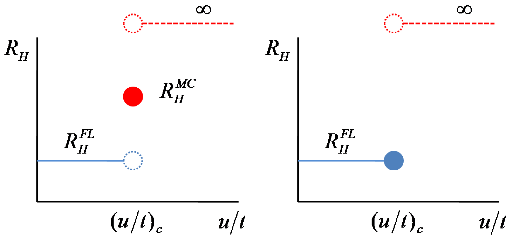
In this paper we propose evidence of electron fractionalization at Mott criticality from the Hall coefficient. An essential feature of the fractionalizaion scenario is appearance of novel charge fluctuations (holons) near the Mott critical point, giving rise to an interesting metallic state in two dimensions. Such charge fluctuations turn out to contribute to the Hall coefficient additionally on top of the Fermi-liquid value given by fermion excitations (spinons). As a result, we uncover two-step jumps in the Hall coefficient at the two dimensional Mott critical point. On the other hand, both DMFT and SB-MIT allow only one-step jump from the Fermi-liquid value to infinity at the Mott critical point. See Fig. 1.

A scaling theory for fermions has been proposed near Mott criticality based on an ansatz of electron fractionalization, where the scaling expression of the spectral function is determined by both the dynamical critical exponent and the anomalous dimension of fermions [19]. Although this scaling theory serves a convenient framework for quantum criticality in thermodynamics and transport, it is difficult to find such critical exponents in the Fermi-surface problem [20, 21], where they are introduced phenomenologically. This difficulty does not arise in the Hall coefficient, not renormalized by strong correlations, thus suggesting an undisputable evidence for electron fractionalization as the mechanism of the Fermi-surface reconstruction.

We start from the Hubbard model

$c_{i\sigma}$ is an electron field, and $n_{i\sigma}=c_{i\sigma}^{\dagger}c_{i\sigma}$ is its density. $t$ is a hopping parameter, and $u$ is an interaction strength at site $i$. In this study we focus on the case of two spatial dimensions.

A way to describe electron fractionalization is to extract out collective charge dynamics explicitly from correlated electrons, referred as the slave-rotor representation [22, 23]. Such charge fluctuations are identified with zero sound modes in the case of short range interactions while plasmon modes in the case of long range interactions. Actually, one can check that the dispersion of the rotor variable is the same as that of such collective charge excitations. The Mott transition is described by gapping of rotor excitations in the slave-rotor theory.

The slave-rotor theory is based on decomposition of an electron field as follows $c_{i\sigma}=e^{-i\theta_{i}}f_{i\sigma}$, where $e^{-i\theta_{i}}$ is a holon field to carry an electron charge, and $f_{i\sigma}$ is a spinon field to do an electron spin. Resorting to this fractionalization scenario, one can rewrite the Hubbard model in terms of holons and spinons, interacting via gauge fluctuations. Gauge-field excitations are associated with collective spin fluctuations, differentiated from those in the spin-fermion model [18]. Performing the continuum approximation, we reach the following expression for the Mott transition

where the last term with the field strength tensor $f_{\mu\nu}=\partial_{\mu}a_{\nu}-\partial_{\nu}a_{\mu}$ describes the Maxwell dynamics of gauge fluctuations, and the gauge-matter coupling constant is denoted as $g$. $m_{f(b)}$ is the band mass of spinons (holons). A detailed derivation of this procedure can be found in Refs. [22, 23].

This effective U(1) gauge theory has been discussed in the Eliashberg framework, where self-energy corrections of spinons, holons, and gauge fields are incorporated self-consistently, but vertex corrections are neglected [24, 25]. Integrating over both spinons and holons, one finds an effective action for gauge fluctuations

where multi-scale quantum criticality is uncovered from two dynamical critical exponents, $z=1$ from critical dynamics of holons and $z=3$ from particle-hole excitations near the Fermi surface of spinons. $\gamma$ is the damping coefficient, proportional to the density of states of spinons, and $\chi$ is the diamagnetic susceptibility of spinons. $\sigma_{\theta}$ is the holon conductivity. Resorting to this gauge propagator, one can evaluate self-energy corrections of spinons and holons self-consistently in each regime. It was shown that the holon self-energy due to gauge fluctuations is not relevant, implying that the Mott transition falls into the 3D-XY universality class [24, 25]. On the other hand, the spinon self-energy gives rise to scaling for thermodynamics and transport in each regime.

In order to evaluate both longitudinal and transverse transport coefficients, we resort to the quantum Boltzman equation approach [26], given by

for spinons and

for holons, where $G_{f(b)}^{<}(k,\omega)$ and $\Sigma_{f(b)}^{<}(k,\omega)$ are lesser Green’s function and self-energy of spinons (holons), respectively, and $A_{f(b)}(k,\omega)$, $\Gamma_{f(b)}(k,\omega)$, and $\Re\Sigma_{ret}^{f(b)}(k,\omega)$ are imaginary parts of retarded Green’s function, self-energy, and the real part of the retarded self-energy, respectively. $\bm{v}_{k}^{f(b)}$ and $\xi_{k}^{f(b)}$ are velocity and dispersion of spinons (holons), respectively. $n_{f(b)}(\omega)$ is the Fermi-Dirac (Bose-Einstein) distribution function. $\bm{E}$ and $\bm{B}$ are applied electric and magnetic fields while $\bm{\mathcal{E}}$ and $\bm{\mathcal{B}}$ are internal fields related with fractionalization. Since spinons do not carry an electric charge in our assignment, they couple to internal fields only in a gauge invariant way. Equations (4) and (5) are derived in appendix A.

Inelastic scattering with critical fluctuations gives rise to the collision term of the right-hand-side, where each lesser self-energy is given by

$\Im D_{a}(q,\nu)$ is the spectral function of the gauge propagator, given by $z=3$ in the paramagnetic insulating state and $z=2$ at the Mott critical point. $\Im D_{\lambda}(q,\nu)$ is the spectral function of the $\lambda$ propagator, where excitations of $\lambda$ correspond to potential fluctuations for holons in the nonlinear $\sigma$ model description [27]. Such fluctuations are essential, the Mott transition belonging to the XY universality class [24, 25].

These Boltzman equations are simplified further in the Eliashberg approximation, where self-energy corrections do not depend on momentum. Inserting the lesser Green’s function

into the quantum Boltzman equations (4) and (5) with Eq. (6), we find so called vertex distribution functions for spinons and holons

respectively, where $\Omega_{f(b)}=\frac{e\mathcal{B}}{m_{f(b)}c}$ and $\omega_{f(b)}=\frac{eB}{m_{f(b)}c}$ are internal and external cyclotron frequencies, and $\mathcal{E}=\mathcal{E}_{x}+i\mathcal{E}_{y}$ and $E=E_{x}+iE_{y}$ are complex fields. $[\tau_{sc}^{f(b)}(k,\omega)]^{-1}=2\Gamma_{f(b)}(k,\omega)$ is the relaxation rate and $[\tau_{tr}^{f(b)}(k,\omega)]^{-1}$ is the scattering rate associated with the transport time, where the former quantity is obtained from the Eliashberg calculation, and the latter is found with vertex corrections, thus a gauge invariant quantity. A detailed procedure on how to solve quantum Boltzman equations is presented in appendix B.

Inserting these vertex-distribution functions into expressions for currents, we obtain

where $\rho_{F}^{f}$ and $v_{F}^{f}$ are the density of states and Fermi velocity of spinons with a positive numerical constant $\mathcal{C}_{f}$, and $\mathcal{C}_{b}$ is a positive number given by a function of temperature and the ratio $u/t$. $\mathcal{C}_{b}$ is a universal number at the Mott critical point, and it vanishes in the paramagnetic insulator.

Internal magnetic fields are shifted as

determined from the gauge invariance [28]. Another condition for the gauge invariance is the back-flow constraint,

implying that the total internal current should vanish [29]. Then, we reach the final expression for the Hall resistivity

It is important to notice that the transport time does not appear, implying that renormalization of the Hall conductivity due to quantum corrections is cancelled by that of the square of the longitudinal conductivity. A derivation is shown in appendix C.

In the Fermi liquid phase ($u<u_{c}$) holon condensation gives rise to $\chi_{b}\rightarrow\infty$ [28]. Then, we find $\rho_{xy}(T)\approx\frac{\omega_{f}}{e^{2}\mathcal{C}_{f}\rho_{F}^{f}v_{F}^{f2}}$, which coincides with that of the Fermi liquid state. On the other hand, $\chi_{f}\gg\chi_{b}$ results both at the Mott critical point and in the paramagnetic insulator. Then, we obtain $\rho_{xy}(T)\approx\frac{\omega_{b}}{e^{2}\mathcal{C}_{b}}$, resulting from only holons. In the insulating phase we see $\mathcal{C}_{b}\rightarrow 0$. See appendix D. As a result, we obtain $\rho_{xy}(T\rightarrow 0)\rightarrow\infty$. However, it is not the case at the critical point, where the critical dynamics of holons is characterized by their own conductivity. $\mathcal{C}_{b}$ is given by a constant, leading the Hall coefficient at the Mott critical point to differ from the Fermi-liquid value.

Integrating over spinon excitations, we obtain an effective field theory for critical holon dynamics with the $z=2$ gauge dynamics given by Eq. (3) and the $z=1$ $\lambda$ dynamics $D_{\lambda}(q,i\Omega)=\frac{1}{\kappa_{\theta}\sqrt{\Omega^{2}+q^{2}}}$, where $\kappa_{\theta}$ is associated with the compressibility of critical holons. As discussed in Refs. [24, 25], the $z=2$ gauge dynamics does not affect the holon dynamics, preserving the 3D-XY universality class to allow the universal conductivity [30, 31] at the two dimensional Mott critical point. This gives a universal number to $\mathcal{C}_{b}$, resulting in the universal jump for the Hall coefficient at the Mott critical point. On the other hand, if spinons are in the diffusive regime, the gauge dynamics is given by $D_{a}(\bm{q},i\Omega)=\frac{1}{\sigma_{f}|\Omega|+\sigma_{\theta}q}$ with the dc spinon conductivity $\sigma_{f}$. Such gauge fluctuations will affect the holon dynamics, and the Mott transition does not belong to the XY universality class any more. Then, the universal conductivity depends on the damping coefficient $\sigma_{f}$, thus $\mathcal{C}_{b}$ becomes a function of disorder and the density of states of spinons. The Hall coefficient does not become universal. However, it must be different from the Fermi-liquid value, giving rise to two-step jumps in the Hall coefficient at the Mott critical point.

We claim that the (universal) jump in the Hall conductivity will not arise from either the DMFT framework or SB-MIT theory. As revealed in the quantum Boltzman equation approach, the Hall coefficient does not renormalize due to quantum corrections. Recalling that the configuration of a Fermi surface is unchanged at the Mott critical point in these frameworks, the Hall coefficient of the Mott critical point remains the same as the Fermi-liquid value, and jumps to an infinite directly in either the paramagnetic insulator or an antiferromagnetic insulator (Fig. 1).

One may criticize the assumption for the existence of the paramagnetic insulating state, referred as a spin liquid phase [32]. Although metal-insulator transitions are usually involved with symmetry breaking, such an insulating phase has been proposed in the DMFT framework [33] and the gauge theory scenario [8, 34]. In particular, such a state has been observed by various numerical simulations when geometrically frustrated lattices are considered to prohibit magnetic ordering [35]. However, the stability of the spin liquid state is not an important issue in our study. The point is whether electron fractionalization appears or not at the Mott critical point. If it occurs, the two-step jumps should be shown in the Hall coefficient, independent of the nature of an insulating phase.

In this study we discussed how the spin-charge separation scenario near two dimensional Mott criticality can be verified from the Hall coefficient. An essential point is that a novel metallic state emerges at the Mott critical point, described by critical dynamics of holon excitations. As a result, such charge fluctuations contribute to the Hall coefficient additionally on top of the Fermi liquid value, given by spinon excitations. Interestingly, the jump of the Hall coefficient turns out to be universal in the clean limit, given by the 3D-XY universality class of critical holon dynamics. We claim that the two-step behavior of the Hall coefficient (Fig. 1) can be regarded as a fingerprint of electron fractionalization because either the dynamical mean-field theory or symmetry-breaking metal-insulator transition allows only one-step jump.

One cautious person may criticize that the behavior of the Hall coefficient depicted in the right hand side of Fig. 1 and that of the left hand side do not differ from each other in the experimental point of view, if the Mott transition occurs really just at a critical point instead of a critical region. In this respect the behavior of the Hall coefficient at finite temperatures may be essential. Since the jump in the Hall coefficient is given by novel metallicity of holon dynamics, we are suspecting an interesting scaling behavior in $U/T$ and $H/T$ for the Hall-coefficient jump, where $U$ is a tuning parameter, here the Hubbard-$U$, and $H$ is externally applied magnetic field. In particular, the scaling exponent will be given by that of the 3D-XY universality class in the clean limit. Unfortunately, we cannot find any previous researches on the scaling behavior of the Hall coefficient in the superfluid to Mott insulator transition of the bosonic Hubbard-type model. This will be an interesting and important future work.

This work was supported by the National Research Foundation of Korea (NRF) grant funded by the Korea government (MEST) (No. 2011-0074542).

References

• [1] M. R. Norman, Physics 3, 86 (2010).
• [2] N. Doiron-Leyraud et al., Nature (London) 447, 565 (2007).
• [3] E. A. Yelland et al., Phys. Rev. Lett. 100, 047003 (2008); A. F. Bangura et al., Phys. Rev. Lett. 100, 047004 (2008); C. Jaudet et al., Phys. Rev. Lett. 100, 187005 (2008); S. E. Sebastian et al., Nature (London) 454, 200 (2008); B. Vignolle et al., Nature (London) 455, 952 (2008); A. Audouard et al., Phys. Rev. Lett. 103, 157003 (2009).
• [4] M. Imada, A. Fujimori, and Y. Tokura, Rev. Mod. Phys. 70, 1039 (1998).
• [5] D. LeBoeuf et al., Phys. Rev. B 83, 054506 (2011); P. M. C. Rourke et al., Phys. Rev. B 82, 020514 (2010); J. Chang et al., Phys. Rev. Lett. 104, 057005 (2010).
• [6] S. Paschen et al., Nature 432, 881 (2004).
• [7] S. Friedemann et al., PNAS 107, 14547 (2010).
• [8] P. A. Lee, N. Nagaosa, and X.-G. Wen, Rev. Mod. Phys. 78, 17 (2006).
• [9] A. Georges, G. Kotliar, W. Krauth, and M. J. Rozenberg, Rev. Mod. Phys. 68, 13 (1996).
• [10] H. v. Lohneysen, A. Rosch, M. Vojta, and P. Wolfle, Rev. Mod. Phys. 79, 1015 (2007); P. Gegenwart, Q. Si, and F. Steglich, Nature Physics 4, 186 (2008).
• [11] K.-S. Kim, A. Benlagra, and C. Pépin, Phys. Rev. Lett. 101, 246403 (2008).
• [12] K.-S. Kim and C. Pépin, Phys. Rev. Lett. 102, 156404 (2009).
• [13] Ki-Seok Kim and C. Pépin, Phys. Rev. B 81, 205108 (2010); K.-S. Kim and C. Pépin, Phys. Rev. B 83, 073104 (2011).
• [14] Minh-Tien Tran, A. Benlagra, C. Pépin, and Ki-Seok Kim, in preparation.
• [15] I. Paul, C. Pépin, and M. R. Norman, Phys. Rev. Lett. 98, 026402 (2007); I. Paul, C. Pépin, M. R. Norman, Phys. Rev. B 78, 035109 (2008).
• [16] C. Pépin, Phys. Rev. Lett. 98, 206401 (2007); C. Pépin, Phys. Rev. B 77, 245129 (2008).
• [17] Q. Si, S. Rabello, K. Ingersent, and L. Smith, Nature (London) 413, 804 (2001).
• [18] T. Moriya and J. Kawabata, J. Phys. Soc. Jpn. 34, 639 (1973); T. Moriya and J. Kawabata, J. Phys. Soc. Jpn. 35, 669 (1973); J. A. Hertz, Phys. Rev. B 14, 1165 (1976); A. J. Millis, Phys. Rev. B 48, 7183 (1993); A. Rosch, A. Schröder, O. Stockert, and H. v. Löhneysen, Phys. Rev. Lett. 79, 159 (1997).
• [19] T. Senthil, Phys. Rev. B 78, 035103 (2008).
• [20] Sung-Sik Lee, Phys. Rev. B 80, 165102 (2009).
• [21] Max A. Metlitski and S. Sachdev, Phys. Rev. B 82, 075127 (2010).
• [22] S. Florens and A. Georges, Phys. Rev. B 70, 035114 (2004).
• [23] Minh-Tien Tran and Ki-Seok Kim, Phys. Rev. B 83, 125416 (2011).
• [24] T. Senthil, Phys. Rev. B 78, 045109 (2008).
• [25] D. Podolsky, A. Paramekanti, Y.-B. Kim, and T. Senthil, Phys. Rev. Lett. 102, 186401 (2009).
• [26] G. D. Mahan, Many-Particle Physics 3th ed. (Kluwer Academic/Plenum Publishers, New York, 2000).
• [27] In order to describe the Mott transition from a spin liquid state to a Fermi liquid phase, it is convenient to resort to the description of the nonlinear σ\sigma model. Performing ei​θ𝒙→ψ𝒙e^{i\theta_{\bm{x}}}\rightarrow\psi_{\bm{x}} with the unimodular constraint |ψ𝒙|2=1|\psi_{\bm{x}}|^{2}=1, one can rewrite the effective Lagrangian Eq. (2) as follows
Z=∫Dψ𝒙Df𝒙​σDλ𝒙Dφ𝒙D𝒂𝒙e−∫0βdτ∫d2𝒓ℒ,\displaystyle Z=\int D\psi_{\bm{x}}Df_{\bm{x}\sigma}D\lambda_{\bm{x}}D\varphi_{\bm{x}}D\bm{a}_{\bm{x}}e^{-\int_{0}^{\beta}d\tau\int d^{2}\bm{r}{\cal L}},
ℒ=f𝒙​σ†(∂τ−μ−iφ𝒙)f𝒙​σ+12​mf|(∇−i𝒂𝒙)f𝒙​σ|2\displaystyle{\cal L}=f_{\bm{x}\sigma}^{\dagger}(\partial_{\tau}-\mu-i\varphi_{\bm{x}})f_{\bm{x}\sigma}+\frac{1}{2m_{f}}|(\bm{\nabla}-i\bm{a}_{\bm{x}})f_{\bm{x}\sigma}|^{2}
−12​u​(ψ𝒙∗​∂τψ𝒙−i​φ𝒙)2+12​mb​|(∇−i​𝒂𝒙)​ψ𝒙|2\displaystyle-\frac{1}{2u}(\psi^{*}_{\bm{x}}\partial_{\tau}\psi_{\bm{x}}-i\varphi_{\bm{x}})^{2}+\frac{1}{2m_{b}}|(\bm{\nabla}-i\bm{a}_{\bm{x}})\psi_{\bm{x}}|^{2}
+i​λ𝒙​(|ψ𝒙|2−1)+14​g2​fμ​ν​fμ​ν.\displaystyle+i\lambda_{\bm{x}}(|\psi_{\bm{x}}|^{2}-1)+\frac{1}{4g^{2}}f_{\mu\nu}f_{\mu\nu}.
λ𝒙\lambda_{\bm{x}} is introduced to keep the rotor constraint, where λ𝒙\lambda_{\bm{x}} fluctuations play an important role in the self-energy correction of the ψ𝒙\psi_{\bm{x}} field.
• [28] P. A. Lee and N. Nagaosa, Phys. Rev. B 46, 5621 (1992); N. Nagaosa and P. A. Lee, Phys. Rev. Lett. 64, 2450 (1990).
• [29] L. B. Ioffe and A. I. Larkin, Phys. Rev. B 39, 8988 (1989).
• [30] M. P. A. Fisher, G. Grinstein, and S. M. Girvin, Phys. Rev. Lett. 64, 587 (1990).
• [31] M.-C. Cha, M. P. A. Fisher, S. M. Girvin, M. Wallin, A. Peter Young, Phys. Rev. B 44, 6883 (1991).
• [32] L. Balents, Nature 464, 199 (2010).
• [33] B. Kyung and A.-M. S. Tremblay, Phys. Rev. Lett. 97, 046402 (2006); O. Parcollet and G. Biroli, and G. Kotliar, Phys. Rev. Lett. 92, 226402 (2004).
• [34] S.-S. Lee and P. A. Lee, Phys. Rev. Lett. 95, 036403 (2005); A. V. Chubukov, S. Sachdev, and J. Ye, Phys. Rev. B 49, 11919 (1994).
• [35] T. Yoshioka, A. Koga, and N. Kawakami Phys. Rev. Lett. 103, 036401 (2009); T. Koretsune, Y. Motome, and A. Furusaki J. Phys. Soc. Jpn. 76, 074719 (2007); T. Watanabe, H. Yokoyama, Y. Tanaka, J.-I. Inoue, J. Phys. Soc. Jpn. 75, 074707 (2006); J. Liu, J. Schmalian, and N. Trivedi, Phys. Rev. Lett. 94, 127003 (2005); H. Morita, S. Watanabe and M. Imada, J. Phys. Soc. Jpn. 71, 2109 (2002).